Fixed effects inference for clustered data in Gaussian linear models

(1)

FIXED EFFECTS INFERENCE FOR CLUSTERED DATA IN

GAUSSIAN LINEAR MODELS

Jacqueline L. Johnson

A dissertation submitted to the faculty of the University of North Carolina at Chapel Hill in partial fulfillment of the requirements for the degree of Doctor of Public Health in the Department of Biostatistics, School of Public Health.

Chapel Hill 2007

Approved by:

Co-Advisor: Diane J. Catellier

Co-Advisor: Keith E. Muller

Reader: Lisa M. LaVange

Reader: David M. Murray

(2)

c

2007

(3)

ABSTRACT

Jacqueline L. Johnson: Fixed Effects Inference for Clustered Data In Gaussian Linear Models (Under the direction of Dr. Diane J. Catellier and Dr. Keith E. Muller)

Important public health research often requires the use of community based studies due

to logistical, ethical and cost constraints. Such designs require special methods of analysis.

Gaussian clustered data are often analyzed with either a mixed effects linear model on individual

level data or two-stage analysis of cluster means. For data with a large number of clusters and

large number of observations within each cluster, both techniques provide unbiased hypothesis

tests. In small samples with unbalanced data, however, even moderate imbalance in cluster size

across treatment groups can bias hypothesis tests in the two stage analysis of cluster means.

The use of large sample approximations for one-stage mixed model test statistics for analysis

of small, unbalanced clustered experiments may also lead to inaccurate hypothesis tests.

I derived a formulation of quadratic form theory which leads to a method to obtain exact

test size for hypothesis tests in the two stage model. This theory is used in an enumeration

study of type I error for a test of treatment difference in the two stage analysis of cluster means

where means are either unweighted or weighted by their cluster size. These enumerations focus

on scenarios of imbalance common to non-randomized cluster data settings.

Next I performed a simulation study of type I error for a test of treatment difference in both

the analysis of individual level data and of cluster means for scenarios of imbalance common to

randomized clustered data trials. Ten methods were considered; of these, a two stage analysis

of cluster means with means weighted by their theoretical variance controlled type I error under

the most cases. In this analysis, the weights contain restricted maximum likelihood estimates

of variance components estimated from the individual level data and are constrained to be

positive.

Many current clustered data studies currently show a misalignment between power

calcu-lations and data analysis; that is, the power analysis is done for a simplified version of the

(4)

actual test computed. I showed how to perform an appropriate and valid power analysis for

(5)

ACKNOWLEDGMENTS

First, I would like to thank my advisors, Diane Catellier and Keith Muller, for their

men-torship and friendship throughout the writing of this dissertation. I would also like to thank

Keith Muller for his leadership, caring, and encouragement throughout all stages of my graduate

education. I am also grateful to the members of my committee, Lisa LaVange, David Murray,

and John Preisser, for their helpful ideas and comments. I would also like to thank Robert

Hamer, Michael Schell, Larry Kupper, and Ruth Marinshaw for their guidance and friendship

during specific phases of my education. Finally, I am very grateful to my family and friends for

their continual love and support, without which I would have never attempted nor finished this

dissertation and doctoral program.

(6)

TABLE OF CONTENTS

LIST OF TABLES . . . viii

LIST OF FIGURES . . . ix

1 Introduction and Literature Review 1 1.1 Introduction . . . 1

1.2 Aims . . . 3

1.3 Notation . . . 5

1.4 Statement of Models and Hypothesis . . . 8

1.5 Literature Review . . . 10

1.6 Motivating Data Example . . . 16

2 Exact Type I Error in the Two Stage Analysis of Cluster Means 20 2.1 Introduction . . . 20

2.2 Hypothesis Testing for Cluster Means . . . 22

2.3 Theoretical Result to Compute Probabilities Under Violation of Assumptions . . 26

2.4 Description of Enumerations . . . 27

2.5 Results of Enumeration Study . . . 29

2.6 Conclusions and Recommendations . . . 32

2.7 Proof . . . 33

3 Comparison of Type I Error for One Stage and Two Stage Models 43 3.1 Introduction . . . 43

3.2 Statement of Models and Hypothesis . . . 44

3.3 Hypothesis Testing for Clustered Data with Balanced Cluster Sizes . . . 47

3.4 Hypothesis Testing for Clustered Data with Unbalanced Cluster Sizes . . . 51

3.5 Description of Simulations . . . 53

3.6 Results of Simulation Study . . . 57

(7)

4 Power Analysis for Continuing a Longitudinal Cluster Sample 80

4.1 Introduction . . . 80

4.2 Literature Review . . . 81

4.3 Performing the Power Analysis . . . 84

4.4 Data Example . . . 88

4.5 Further Remarks . . . 89

5 Summary and Future Research 91 Bibliography . . . 94

(8)

LIST OF TABLES

1.1 Notation in This Document Compared to Traditional Mixed Model Notation . . 7

1.2 Summary of Non Matrix Notation . . . 7

1.3 Type I Error for One Stage and Two Stage Analyses . . . 19

2.1 Summary of Non Matrix Notation . . . 34

2.2 Type I error over all cases and byρ,m1×m2 and m2/m1 . . . 35

2.3 Type I error by ¯n1×n¯2 and ¯n2/n¯1 . . . 36

2.4 Type I error by r1×r2 and r2/r1 . . . 37

2.5 Type I error by m2/m1×n¯2/n¯1 . . . 38

2.6 Type I error by m2/m1×n¯2/n¯1 (cont.) . . . 39

3.1 Number of convergent scenarios for tests 2, 4, and 10, by ρand m1×m2 . . . 62

3.2 Number of scenarios with a negative variance component estimate, by ρ and m1×m2 . . . 63

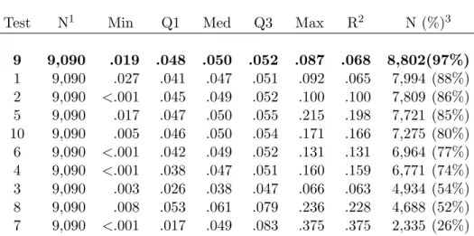
3.3 Type I error over all cases . . . 64

3.4 Number (%) of total (N=9,090) cases where test i (down) is biased and test j (across) is unbiased. . . 65

3.5 Difference in Number (i, j) and Number (j, i) from Table 3.4. . . 65

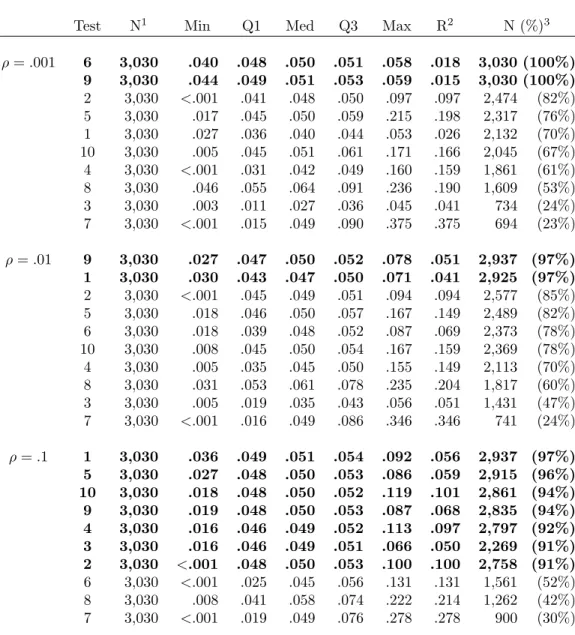
3.6 Type I error by ρ . . . 66

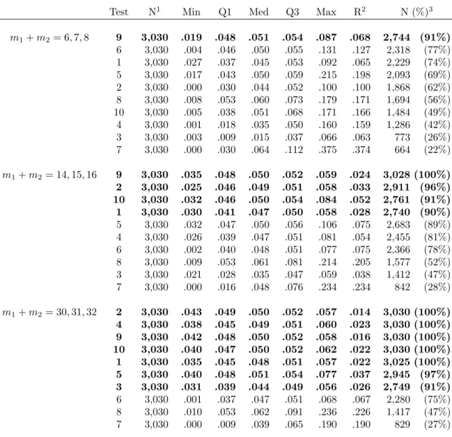
3.7 Type I error by m1+m2 . . . 67

3.8 Type I error for selected scenarios of balance . . . 68

(9)

LIST OF FIGURES

2.1 Type I Error for ρ×m1×m2×n¯1×n¯2 - Analysis of Unweighted Means . . . . 40

2.2 Type I Error forρ×m1×m2×n¯1×n¯2 - Analysis of Means Weighted By Cluster Size . . . 41

2.3 Type I Error for ρ×m1×m2×n¯1×n¯2 - Comparison of Weights . . . 42

3.1 Type I Error for Test 1 by ρ,m1,m2, ¯n1, and ¯n2 . . . 70

3.10 Type I Error for Test 10 byρ,m1,m2, ¯n1, and ¯n2 . . . 79

4.1 Power as a Function Mean Difference . . . 90

(10)

Chapter 1

Introduction and Literature Review

1.1 Introduction

The term “clustered data” commonly refers to data collected on individuals who are nested

within a specific geographical or civil unit, e.g., children within schools, employees within

work-sites, or patients within physician practices. Clustered designs are often intentionally used to

study the relationship of characteristics at the individual and cluster level on the response of

interest. Many public health studies also require the use of clustered instead of fully

inde-pendent data collection designs due to logistical, ethical and cost constraints. For randomized

studies, the trials through which clustered data arise are usually called group randomized trials

or cluster randomized trials [7, 24]. Such trials have been performed broadly across areas of

medicine and public health, most notably in the areas of smoking prevention, physical activity

promotion, occupational safety, nutrition, dentistry, and health policy. Clustered designs also

arise with the framework of sample surveys, though we do not consider these here. Specific

features of clustered data are: the independent sampling unit is the cluster; characteristics of

individuals within a cluster tend to be correlated, equally among each other; and the

explana-tory variable of primary scientific interest, e.g., treatment group, is applied at the cluster level,

while data are collected at the individual or within-cluster level.

Many continuous outcomes of interest in public health studies with clustered data have

an approximate Gaussian distribution. The analysis of Gaussian clustered data within the

framework of a univariate or repeated measures mixed linear model with Gaussian errors is

discussed in this dissertation. For simplicity, in this paper, we refer to the explanatory variable

(11)

groups applies to any fixed cluster level explanatory variable.

If clustered data are balanced so that each cluster contributes the same number of

observa-tions, and if data have a common within-cluster correlation and individual error variance across

treatment groups, then the set of outcome cluster means are sufficient statistics for inference

about treatment group means. That is to say that knowledge of the individual level outcome

data gives no additional information about the treatment means over that given by the outcome

cluster means. This is true even when the outcome of interest depends on additional covariates

other than treatment group, so long as the relationship between the outcome and covariates

is the same across treatment groups. With the addition of covariates other than treatment

group, knowledge of outcome cluster means and cluster covariate averages suffices for inference

about treatment group. Sufficiency of cluster averages for inference about treatment groups is

due to the special compound symmetric covariance structure of clustered data.

If data are unbalanced, so that a different number of observations is taken in each cluster,

then the set of outcome cluster means (with, also, cluster covariate averages, if applicable)

are no longer sufficient statistics for inference about treatment group means. This means

that inference conducted on cluster means with, potentially, also cluster covariate averages, is

different than that conducted on individual level data.

Varnellet al.[35] showed that current researchers analyze both cluster means and individual

level data. They reviewed group randomized trials published in the American Journal of

Public Health and Preventative Medicine from 1998 to 2002, and showed that of the 47 trials

that employed at least one statistical analysis appropriate for group randomized trials (some

analyses did not account for the correlation within clusters at all), 15 (32%) analyzed cluster

means or another summary statistic and 32 (68%) analyzed individual level data. Analysis

of cluster means is often called a “two-stage” model, whereby the cluster means are computed

first, often adjusted for covariates through a preliminary model excluding treatment group, and

cluster means are the values of the response in a linear model at the second stage [24, p. 112].

Analysis of the individual level data is often called a “one-stage” analysis, where correlated

individual level data are analyzed via a mixed effects linear model [24, p. 112].

In this dissertation, we confine interest to Gaussian linear models that include a single

fixed effect (e.g., treatment), a random cluster effect, and the usual residual random error.

(12)

Such a model is called a two-variance components model [14], two-way nested [27], multi-level

[8] or hierarchical model [2], or a one-way mixed model [14]. Though analysis of data from

epidemiological studies typically adjust for additional fixed covariates or levels of clustering, it

is an important first step to explore the properties of hypothesis tests in the simplest model

with no covariates and one level of clustering.

If data have a common within-cluster correlation and common individual error variance,

and if data have balanced cluster sizes, both the one-stage and two-stage approaches give the

same hypothesis test for the fixed effects [9]. Further, this test is the uniformly most powerful

size-α test and has exact null and non-null distributions. Also, this test statistic is derived

from closed formed expressions for the maximum likelihood estimates for the fixed effects and

variance components, which have known distributions.

If any of the previous conditions about common variance, correlation, or cluster size do not

hold, the one-stage and two-stage analysis approaches lead to different tests. No uniformly

most powerful size-αtest for the fixed effects exist; the unbalanced versions of the test statistics

used for balanced data now have only approximate distributions; and closed form expressions

for estimates of variance components are no longer available.

Research is needed to study the distributional properties of the hypothesis test statistics for

fixed effects in the one-stage and two-stage analysis of unbalanced clustered data. In Chapter

2, enumerations of type I error for hypothesis tests for fixed effects in the two-stage model

are presented. Situations of imbalance common to non-randomized clustered data settings are

considered there. In Chapter 3, simulations of type I error for hypothesis tests for fixed effects

in both the one-stage and two-stage models are presented. These emphasize designs common

to group randomized trials. In Chapter 4, a method is described which computes power for

the hypothesis test which best controlled type I error in Chapter 3. The aims of these chapters

are described in more detail in the next section.

1.2 Aims

1.2.1 Chapter 2, Paper 1

1. Show how to write the null and non-null distributions of the two-stage cluster means

(13)

chi-square random variables. Probabilities for this sum can be computed using Davies

[4] algorithm. In the null case, these probabilities are exact; in the alternative case, they

are exact given a well-approximated critical value.

2. Produce a SAS/IML module that computes probabilities from the distribution described

in Aim 1.

3. Use the modules in Aim 2 to perform an enumeration study showing the bias in type

I error for the two-stage cluster means model test statistic for a range of scenarios of

imbalance in number of observations per cluster and number of clusters common to non

randomized clustered data studies. We will consider the two-stage cluster means model

test statistic with cluster means unweighted and weighted by cluster size.

1. Conduct simulations of type I error for the one-stage individual level and two-stage

clus-ter means model test statistics for a variety of conditions of imbalance common to group

randomized trials. Ten tests are considered. For the one-stage model, degrees of

free-dom will be calculated (1-2) by the method of Kenward and Roger [13] and (3-4) as the

number of clusters minus the number of treatment groups. Both methods will include

simulations with variance components unconstrained and constrained to be positive. For

the two-stage model, the following weight matrices will be considered: (5) unweighted,

(6) weighted by cluster size, (7) weighted by inverse of cluster size, (8) weighted by the

inverse of the sample variance of each cluster mean, and (9-10) weighted by the inverse of

the theoretical variance of each cluster mean, with variance components estimated from

the entire data. The last two stage analysis will be performed with variance components

unconstrained and constrained to be positive.

2. Suggest which of the tests in Aim 1 controls type I error for the most scenarios of

imbal-ance.

3. Suggest conditions of imbalance under which each test as well as more than one test

provides an unbiased test for the fixed effects.

(14)

1. Show how to compute power for unbalanced clustered data in the two stage analysis of

cluster means with means weighted by the inverse of estimates of their theoretical variance.

2. Illustrate use of this method using data from a study on adolescent drinking behavior.

In the remainder of this chapter, I discuss literature relevant to each of these topics; material

for each paper is developed in more detail in Chapters 2, 3, and 4. Chapter 2, 3, and 4 were

written as stand alone papers, and so repeat some of the literature review presented in this

chapter.

1.3 Notation

1.3.1 Matrix Notation

This section describes the notational conventions used in this document. Lower case bold

indicates a (column) vector, upper case bold a matrix. Upper case italics indicates a

non-matrix random variable. Matrix notation dominates over random variable notation, so that

randomness of a matrix must be inferred from context.

We follow the notation of McCulloch and Searle [19], Appendix M, Section 3, to conveniently

denote stacked column vectors and diagonal matrices with similar notation. Define the indices

iandj such thati= 1, ..., aandj= 1, ..., b. Letu=_cuij denote the stacked column vector

u, where u=u0₁₁ u0₁₂ . . . u_ij0 . . . u0_ab 0. LetU =_dUij denote the diagonal matrix

U with diagonal elements U11,U12, ...,Uij, ...,Uab. These notations are identical except for

the subscript on the opening brace; the subscript c denotes a stacked column vector and the

subscriptddenotes a diagonal matrix.

Kronecker product multiplication of matrix A by matrix B is denoted by A⊗B,where

A⊗B= 

       

a11B a12B ... a1aB

a21B a22B ... a2aB

... ... ... .. ab1B ab2B ... aabB



       

,

andaij is the element in thei-th row andj-th column of matrixA. All other matrix operators

(15)

1.3.2 Distributions

Let x∼ N_N(µ,Σ) indicate that the vectorx (N ×1) follows an N-variate normal

distri-bution with mean vector µand covariance matrix Σ. Let X ∼ F(ν1, ν2, ω) indicate that the

random variable X has a noncentral F distribution withν1 numerator degrees of freedom, ν2

denominator degrees of freedom, and noncentralityω. LetX∼χ2(ν1, ω) indicate thatX has

a non-central chi-square distribution withν1degrees of freedom and noncentralityω. With zero

noncentralities, both the noncentral F and χ2 distributions reduce to central versions. Kotz

et al. [17] gives detailed information about these distributions.

1.3.3 Data Indices and Model Notation

Theory and results in this document are discussed within the framework of the general linear

mixed model and the general linear univariate model. Notational conventions from these areas

are used heavily in this document, e.g., Verbeke and Molenberghs [36] or Muller and Stewart [23].

Such notation can differ from other notational schemes that also would have been defensible,

namely, that used in any of multivariate, hierarchical, or multi-level linear models or in the

field of group or cluster randomized trials. When necessary for clarity, notation from these

fields must be employed. In particular, because this dissertation focuses heavily on properties

of balanced versus unbalanced data, we make different choices of notation for total number of

observations, number of independent sampling units, and number of observations per cluster,

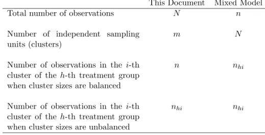
than those usually made in traditional mixed model notation. Table 1.1 summarizes these

notational differences. Table 1.2 summarizes the notation used in this document to describe

the structure of clustered data.

(16)

Table 1.1: Notation in This Document Compared to Traditional Mixed Model Notation

This Document Mixed Model

Total number of observations N n

Number of independent sampling units (clusters)

m N

Number of observations in the i-th

cluster of the h-th treatment group

when cluster sizes are balanced

n nhi

Number of observations in the i-th

cluster of the h-th treatment group

when cluster sizes are unbalanced

nhi nhi

Table 1.2: Summary of Non Matrix Notation

Symbol Definition

Indicies

h= 1, . . . , g Indexes treatment groups

i= 1, . . . , mh Indexes clusters within treatment group

j= 1, . . . , nhi Indexes observations within cluster

Numbers of Clusters and Observations

g Number of treatment groups

mh Number of clusters in treatment grouph

m=Pg_h₌₁mh Total number of clusters

nhi Number of observations within a cluster when

clus-ter sizes are unequal

n Number of observations within a cluster when

clus-ter sizes are equal

nh=Pmi=1h nhi Number of observations in treatment grouph

N =Pg_h₌₁Pmh

i=1nhi Total number of observations

Outcome Notation

yhij Outcome for observationj of clusteriin treatment

grouph

y_hi= _n1

hi

Pnhi

j=1yhij Outcome mean for clusteriin treatment grouph

y_h= _m1

h

Pmh

i=1

Pnhi

(17)

1.4 Statement of Models and Hypothesis

1.4.1 One-Stage Model

Define a linear model for continuous Gaussian outcome y₁ that includes fixed effects given

inβ (g×1),a random effect for cluster given inb(m×1),and a random error,e1 (N ×1):

y₁=X1β+Z1b+e1. (1.1)

The matricesX1(N×g) andZ1(N×m) are design matrices for the fixed and random effects,

respectively. This review assumesX1 contains only an effect for treatment group andZ1 only

an effect for cluster.

Vectors or matricesy₁,X1,Z1,ande1 are stacked by treatment group and cluster so that

y₁ =

cy1,hi ,X1=

cX1,hi ,Z1 =

cZ1,hi , ande1 =

ce1,hi . Without loss of generality,

assume the fixed effects design matrixX1 has a cell mean coding for treatment group so that

X1=

d1nh . The design matrix for the random cluster effect isZ1=

d1nhi . When data

have balanced cluster sizes, these simplify toX1 =

d1mhn and Z1 =Im⊗1n.

We assume b∼ Nm 0, σc2Im

independently of e1 ∼ NN 0, σ

2

eIN

so that:

y₁ ∼ N_N(X1β,Σ1) ,

where the covariance matrix Σ1 (N ×N) is compound symmetric and has the form:

Σ1 =σ2cZ1Z01+σ2eIN =

dσ

2

c1nhi1

0

nhi+σ

2

eInhi .

Σ1 may be expressed in terms of the total variance,σ2y, and within cluster correlation, ρ, as:

Σ1 =σ2y

d1nhi1

0

nhiρ+Inhi(1−ρ) ,

where ρ = σ_c2/ σ_c2+σ_e2 and σ_y2 = σ_c2 +σ_e2 or, equivalently, σ_c2 = σ2_yρ and σ_e2 = σ2_y(1−ρ).

Implicit in construction ofΣ1 is the assumption that data across all treatment groups have the

same variance parameters. When data have balanced cluster sizes the covariance matrix Σ1

simplifies to:

Σ1 =Im⊗ σ2c1n10n+σe2In

=Im⊗σ2y

d1n1

0

nρ+In(1−ρ) .

(18)

1.4.2 Two-Stage Model

To transform from a model for individual level data to a model for cluster means,

pre-multiply model (1.1) by the matrix T1 (m×N), where T1 =

d1

0

nhi/nhi . This yields a

model for y₂ (m×1) =T1y1 where:

y₂=X2β+Z2b+e2, (1.2)

and X2 (m×g) = T1X1, Z2 (m×m) = T1Z1, and e2 (m×1) = T1e1. Parameters in β

and bwere not affected by the transformation.

The vector of outcomes, y₂, and of random errors, e2, contain cluster averages, so that

y₂ = _cy_hi and e2 =

cehi . The fixed and random effects design matrices are X2 =

d1

0

nhi/nhi d1nh =

d1mh and Z2 =

d1

0

nhi/nhi d1nhi =Im.

In line with previous assumptions, we assume b ∼ N_m 0, σ_c2Im

independently of e2 ∼

N_m 0, σ2_eT1T01

so that:

y₂∼ N_m(X2β,Σ2) ,

whereΣ2 (m×m) is given by:

Σ2 =T1Σ1T0₁ =_dσ_c2+σ_e2/nhi .

In terms of the alternate parameterization with σ_y2, ρ instead of σ_e2, σ2_c:

Σ2 =σy2

d[1 + (nhi−1)ρ]/nhi .

1.4.3 General Linear Hypothesis

Define a vector of secondary contrast parameters,θ(a×1) =Cβ, whereC(a×g) contains

desired contrasts for the fixed effects. For clustered data y₁ and y₂ in models 1.1 and 1.2,

elements ofθ are linear combinations of cluster means. We study the two-sided general linear

hypothesis (GLH):

H0:θ=θ0 versus H1 :θ6=θ0. (1.3)

In most hypotheses of interest,θ0 =0. Such a hypothesis test describes differences in the fixed

effects only. We do not consider tests for variance components or ratios of variance components

in this dissertation. If θ is estimable, requiringC to have full row rank [rank(C) =a] ensures

(19)

requirement is automatically satisfied ifX is full rank, so that (X0X)−1 exists [21].

1.5 Literature Review

1.5.1 Hypothesis Testing for Clustered Data with Balanced Cluster Sizes

The analysis of clustered data has special properties when data have balanced cluster sizes.

This section describes estimation and hypothesis testing of fixed effects for such balanced data.

In practice, these methods are applied to unbalanced clustered data as well. Section 1.5.2

describes the properties of methods of estimation and hypothesis testing for balanced clustered

data when applied to unbalanced data.

1.5.1.1 Estimation of Fixed Effects for the One Stage Model for Individual Data

Consider the one-stage model for individual level data y₁ ∼ NN(X1β,Σ1) given in model

1.1. When Σ1 is unknown, and therefore contains nuisance parameters which must be

esti-mated, the restricted maximum likelihood (REML) estimator for βis:

b

β₁=

X0₁Σb

−1

1 X1

−1

X0₁Σb

−1

1 y1,

where Σ1b (N ×N) is the REML estimator for Σ1. When individual level clustered data y₁

have balanced cluster sizes, that is, when nhi ≡n for all h,i, the estimator Σ1b can be stated

in terms of a Kronecker product of the same covariance matrix for all clusters. That is,

b

Σ1 =Im⊗

b

σ2

y[1n10nbρ+In(1−ρb)] . Because of this, the inverse ofΣb1 can be written with

the closed form expression:

b

Σ−₁1 =Im⊗ 1

b

σ2

y(1−ρb)

In− b

ρ

[1 + (n−1)ρb]

1n10n

.

For balanced data with no covariates, X1 =

d1mhn , and we can show that X

0

1Σb

−1

1 =

b

σ2_y[1 + (n−1)ρb]

−1

X0₁. Thus, for balanced data:

b

β₁ =

X0₁Σb

−1

1 X1

−1

X0₁Σb

−1

1 y1

=

b

σ2_y[1 + (n−1)ρ_b] −1X0₁X1

−1

b

σ2_y[1 + (n−1)ρ_b] −1X0₁y₁

= X0₁X1

−1

X0₁y₁.

We now have an estimator for the fixed effects that does not depend on the variance components.

That is, for balanced data, the weighted least squares and ordinary least squares estimators of

(20)

βcoincide. Puntanen and Styan [26] and Tian and Wiens [34] gave a comprehensive review of

when weighted or ordinary least squares estimators coincide for general datay∼ N(µ,Σ).

1.5.1.2 Estimation of Fixed Effects for the Two Stage Model for Cluster Means

Consider the two-stage model for cluster means y₂ ∼ N_m(X2β,Σ2) given in model 1.2.

When data are balanced, nhi≡nfor all h, i,so that the cluster means have covariance:

Σ2=Im⊗ σy2/n 1 + (n−1)ρ .

That is, for balanced data, all cluster means have the same variance, andΣ2 can be written as

Σ2 =σ2Im where: σ2 = σy2/n 1 + (n−1)ρ . Independence, normality, and homogeneity

of errors of the cluster means meet the assumptions of the general linear univariate model

(GLUM).

In the general linear univariate model, the best linear unbiased and maximum likelihood

estimator for the fixed effects, β, is:

b

β₂= X0₂X2

−1

X0₂y₂.

1.5.1.3 Equivalence of Estimators from One and Two Stage Models

Matrix algebra allows showing that:

X0₁X1 =

d1

0

mhn d1mhn =

dnmh

X0₁y₁ =_d10_m_h_n _cy₁_,hi =

c

mh

X

i=1

ny_hi

as well as:

X0₂X2=

d10mh

d1mh =

dmh

X2y2= 1

0

mh

{cyhi}=

c

mh

X

i=1

y_hi

.

Thus:

b

β₁ = X0₁X1

−1

X0₁y₁ =_dnmh _c

mh

X

i=1

ny_hi =_cy_h

and:

b

β₂ = X0₂X2

−1

X0₂y₂ =

dmh c

mh

X

i=1

y_hi =

cyh .

That is, for data with balanced cluster sizes, the population treatment means inβare estimated

(21)

1.5.1.4 Hypothesis Test for Fixed Effects

The equivalent estimators given in sections 1.5.1.1 and 1.5.1.2 may be written as

b

β_s= X0_sXs −1

X0_sy_s

wheres= 1,2. Using theory of quadratic forms in normal vectors,βb_s∼ N_g

h

β, σ2(X0_sXs)

−1i

,

whereσ2 = σ2_y/n 1 + (n−1)ρ . Further, an estimator for desired contrasts, θ=Cβ, may

be estimated withbθ_s=Cβb_s, which has distributionbθ_s ∼ N_a

h

θ, σ2C(X0_sXs)−1C0 i

.

Using theory for a general linear univariate model, a uniformly most powerful test size α

for the GLH is given by:

Ts=

b

θs−θ0

0h b

Vbθ_s i−1

b

θs−θ0

/a,

where Vb

b

θs

is the estimated variance of θb_s, that is Vb

b

θs

= _bσ2

h

C(X0_sXs)−1C0 i

. The

quantity bσ

2 _{denotes the restricted maximum likelihood estimator for} _σ2_{, discussed in the next}

section. This test statistic can be shown to have distribution:

Ts∼ F(a, m−g, ω),

whereω = (θ−θ0)0

h

C(X0_sXs)−1C0 i−1

(θ−θ0)/σ2.

1.5.1.5 Estimation of Variance Components

In the two stage analysis of cluster means, variance components σ2_y, ρ or σ_c2, σ_e2 are not

separately estimable so that the linear combination σ2 = σ_y2/n 1 + (n−1)ρ is estimated.

An estimator for σ2 in the two stage analysis of cluster means is:

b

σ2 =y0₂

h

Im−X2 X02X2

−1

X0₂

i

y₂/(m−g).

This estimator can be derived as an restricted maximum likelihood and ANOVA estimator

b

σ2 = SSE2/(m−g), where SSE2 denotes the sums of squares error.

In the one stage analysis of individual level data, though an estimator of the linear

combi-nationσ2 = σ2_y/n 1 + (n−1)ρ =σ2_c+σ_e2/nis needed, current statistical software, designed

for the estimation of parameters of general covariance structures, estimates the variance

com-ponents separately in the parameterization σ2

c, σe2

.

(22)

Define the sums of squares due to cluster and error, respectively, as:

SSC1=y01

h

Z1 Z01Z1

−1

Z1−X1 X01X1

−1

X1

i

y₁

SSE1=y01

h

IN −Z1 Z01Z1

−1

Z0₁

i

y₁.

as well as mean squares due to cluster and error, respectively:

MSC1 = SSC1/(m−g)

MSE1= SSE1/(N −m).

The parameterization σ2

c, σe2

requires estimates of both σ2

c and σ2c to be positive, sinceσc2

andσ2_e are defined as variances. As such, several sources, e.g. Searle [31, p .419], have pointed

out that restricted maximum likelihood estimators forσ2_c and σ2_e are given by:

b

σ_c2 = (MSC1−MSE1)/n

b

σ_e2 = MSE1

when MSC1≥MSE1 (that is, when bσ

2

c is positive) and

b

σ2_c = 0

b

σ2_e = SST1/(N−m)

when MSC1 < MSE1, where SST1 = SSC1+ SSE1 denotes the total sums of squares of the

individual level data. The probability thatσ_b_c2 <0 is:

Pr

b

σ_c2<0 = Pr{F_m−1,N−m<1/[1 +nρ/(1−ρ)]}.

It can be shown that when MSC1 ≥MSE1, the estimator bσ

2 ₌

b

σ2

c +bσ

2

e/n is equivalent to

the best linear unbiased and maximum likelihood estimator obtained in the two-stage analysis;

however this is not the case when MSC1 < MSE1. That is, when MSC1 <MSE1, the linear

combination of restricted maximum likelihood estimators for each of σ_c2 and σ2_e is NOT the

restricted maximum likelihood estimator for the linear combination σ2. The restricted

max-imum likelihood estimator for σ2 is obtained only when variance components estimators are

b

σ_c2 = (MSC1−MSE1)/nand bσ

2

e = MSE1, and the estimator bσ

2

c is allowed to be negative.

Default behavior of SAS PROC MIXED is to constrain estimates of variance components

(23)

1.5.2 Hypothesis Testing for Clustered Data with Unbalanced Cluster Sizes

1.5.3 One Stage Model for Individual Data

When cluster sizes are unbalanced, the weighted least squares estimatorβb₁, given in section

1.5.1.1 as:

b

β₁=

X0₁Σb

−1

1 X1

−1

X0₁Σb

−1

1 y1,

is no longer equivalent to an ordinary least squares estimator. That is, estimation of fixed

effects now requires estimation of the variance components.

Recall that the structure of Σ1 for unbalanced data is:

Σ1 =

dσ

2

c1nhi1

0

nhi+σ

2

eInhi =σ

2

y

d1nhi1

0

nhiρ+Inhi(1−ρ) .

When data are unbalanced, no closed form expressions exist for estimates of the variance

com-ponents in either parameterization; estimates must be obtained by an iterative procedure such

as Newton-Raphson iteration or the EM algorithm [5].

Construction of a hypothesis test for θ = Cβ requires knowledge of the distribution of

b

β₁. The estimator βb₁ is unbiased, so that E

b

β₁

= β; however, no closed form expression

exists for its variance. The common strategy is to approximately estimate this as Vb

b

β₁

≈

X0₁Σb

−1

1 X1

−1

. Kacker and Harville [12] and Dempster et al. [6] pointed out that this

underestimates the true variability in βb₁, since

X0₁Σb

−1

1 X1

−1

is an estimate of the variance

of

∼

β₁ = X0₁Σ−₁1X1

−1

X0₁Σ−₁1y₁ not of the variance of βb₁.

As in hypothesis testing with balanced data, a hypothesis test for the general linear

hypoth-esis is given by the Wald style test statistic:

T1 =

b

θ1−θ0

0h b

Vbθ₁ i−1

b

θ1−θ0

/a.

Since closed form expressions do not exist for the elements ofΣb₁,T₁cannot be written explicitly

as a quadratic form, and thus its exact distribution is unknown. Applying large sample theory

gives T1−→χD 2(a,ω). Given a random variable X with X ∼ F(ν1, ν2,ω), as ν2 −→ ∞,

X−→YD whereY ∼χ2(ν1,ω). For this reason,T1 is usually given an approximate F(a, ν2,ω)

distribution in order to combat the underestimate of the variance ofβb₁. Several methods exist

to estimate the denominator degrees of freedom ofT1. In most cases, none can be shown to be

uniformly superior [18].

(24)

One such method is that proposed by Kenward and Roger [13], who multiply T1 by an

inflation factor to account for the additional variability in Vβb₁

introduced by estimating

Σ1. Satterthwaite [28] style degrees of freedom are then computed for this inflated statistic.

This approximation has not been studied thoroughly in small clustered data settings, and has

been shown to be biased in settings with other types of small sample data [3, 15, 29]. Another

common choice for denominator degrees of freedom is that for the analysis of balanced data,

ddf =m−g.

1.5.4 Two Stage Model for Cluster Means

From section 1.5.1.2, cluster means with balanced cluster sizes may be analyzed via a general

linear univariate model. The general linear univariate model assumesΣ2 is proportional to an

identity matrix, that is Σ2=σ2I, where as before σ2 = σy2/n 1 + (n−1)ρ .

An optimal test for the general linear hypothesis can be derived with the less restrictive

assumption that Σ2 =σ2W−1, that is, that the covariance matrix is known up to a constant

weight matrixW [19]. In this case, the best linear unbiased and maximum likelihood estimator

for the fixed effects is:

b

β₂_w= X0₂W X2

−1

X0₂W y₂.

Withβb₂_w ∼ N_g

h

β, σ2₍_X0

2W X2)

−1i

and thus, bθ₂_w =Cβb₂_w ∼ N_a

h

θ, σ2_C₍_X0

2W X2)

−1

C0i,

a uniformly most powerful size-αtest for the fixed effects can be shown to be given by:

T2w =

b

θ2w−θ0

0h b

Vbθ₂_w i−1

b

θ2w−θ0

/a,

whereVb

b

θ2w

=σb

2

wC(X

0

2W X2)−1C0. The restricted maximum likelihood estimator for σ2

is:

b

σ_w2 =y0₂hW −W X2 X02W X2

−1

X0₂Wiy₂/(m−g).

The statisticT2w has distributionT2w ∼ F(ν1,ν2,ωw), where the noncentrality in the weighted

model isωw = (Cβ−θ0)0

h

C(X0₂W X2)−1C0

i−1

(Cβ−θ0)/σ2.

The exact distribution of the test statistic Tw depends on the assumption that Σ2 can be

written in the form Σ2 =σ2W−1 where W is known. When this doesn’t hold T2w has only

an approximate F distribution. Cluster means derived from unbalanced clustered data with

(25)

estimated; however, many types of weights have W such thatΣ2≈σ2W−1.

If ρ is small and cluster sizes are small,Σ2 ≈ σ2_y _d1/nhi , so that weighting by cluster

sizes is an appropriate choice. Forgetting to invert the weights also may lead researchers

to erroneously weight by the inverse of cluster size. If cluster sizes are not highly variable,

Σ2≈σ2W−1 directly, so an analysis of unweighted means is performed.

In an attempt to estimate the variance components in the weights, data analysts also choose

W =

d[nhi(nhi−1)]/[y

0

hiyhi−nhiy¯1,hi] , the diagonal matrix of inverses of the estimated

sample variance of each cluster mean, or W =

b

σ_y2 _d[1 + (nhi−1)ρb]/nhi

−1

, the diagonal

matrix of the inverse of estimates of the theoretical variance of each cluster mean with variance

components estimated from all the data. Such estimates of variance components from the data

can be constrained to be positive or allowed to be negative.

1.6 Motivating Data Example

The Trial of Activity in Adolescent Girls (TAAG) [32] was designed to evaluate an

inter-vention to reduce the age-related decline in moderate to vigorous physical activity (MVPA) in

middle school girls. The primary endpoint is the mean difference in intensity-weighted minutes

(MET minutes) of MVPA between intervention and control schools. 18 schools were

random-ized to each of intervention and control for a total of 36 schools. Baseline MVPA data were

collected on a sample of 60 6th grade girls per school, then again two years later on a sample

of 120 8th graders per school. Students were sampled at both time points so that data were

not necessarily collected on the same girls at both data collection points. The primary planned

analysis was a two-stage analysis of endpoint MVPA school means adjusted for baseline MVPA

school means. Further details can be found in Stevenset al. [32] and Murrayet al. [25].

One-stage analysis methods on individual level data which properly adjust for baseline values

cannot be conducted on the TAAG data, because the independent cross-sectional sampling

design resulted in incomplete overlap of girls at the two time points. Nonetheless, one can

analyze these data via both two-stage and one-stage methods if baseline data is omitted. We

perform such an analysis below for instructional purposes only; this analysis was not one actually

conducted for this trial.

Suppose the study had pre-planned subgroup analyses by race. The majority of girls in

(26)

the study belonged to three ethnic groups: non-Hispanic white and black, and Hispanic (of any

race). All race groups were not equally represented in all schools. To estimate the treatment

effect among black students, we considered only those schools with at least 2 African American

students, leading to inclusion of 12 intervention schools and 13 control schools. Because the

racial profiles of each school vary widely, each cluster (school) will contribute different numbers

of observations to these data. Clusters sizes in the intervention and control schools were {2,

2, 6, 12, 18, 29, 30, 31, 36, 52, 60, 81}, (mean = 29.9), and {5, 7, 7, 11, 13, 14, 14, 18, 23, 28,

35, 62, 69}, (mean = 23.5), respectively. These cluster sizes are naturally much more variable

that those in the planned primary analysis, but illustrate how extremely unbalanced data can

easily be obtained in an analysis of a subgroup of well-balanced data.

Table 1.3 gives p-values for a test for difference in average MVPA for intervention versus

control schools within the framework of each of the following models :

1. One-stage analysis via a mixed effects model with denominator degrees of freedom

calcu-lated by the method of Kenward and Roger [13].

2. One-stage analysis via a mixed effects model with denominator degrees of freedom equal

tom−g.

3. Two-stage analysis of unweighted cluster means

4. Two-stage analysis of cluster means weighted by cluster size

5. Two-stage analysis of cluster means weighted by the inverse of cluster size

6. Two-stage analysis of cluster means weighted by the inverses of sample variances of each

cluster mean

7. Two-stage analysis of cluster means weighted by the inverse of the theoretical variance,

with variance components estimated with the entire data.

Estimates of variance components for these data were positive.

One stage strategies 1 and 2 and two-stage strategy 7 compute similar, though not equivalent

(27)

cluster size equal to 15 or 40 times the minimum cluster size, two stage approaches 3 - 6 give

widely different results.

(28)

Table 1.3: Type I Error for One Stage and Two Stage Analyses

Estimated Estimated

MVPA Mean (SE) MVPA Mean (SE) Estimated Denom

Analysis Intervention Group Control Group Difference F DF P-value

1 20.35 (0.90) 18.85 (0.90) 1.50 (1.27) 1.18 15.6 0.26

2 20.35 (0.89) 18.85 (0.89) 1.50 (1.26) 1.19 23 0.24

3 20.96 (1.08) 19.66 (1.12) 1.30 (1.56) 0.83 23 0.41

4 20.14 (0.83) 18.49 (0.77) 1.65 (1.13) 1.47 23 0.16

5 22.25 (1.38) 22.93 (1.13) -0.69 (1.79) -0.38 23 0.70

6 18.70 (0.90) 18.23 (0.78) 0.47 (1.19) 0.39 23 0.70

(29)

Chapter 2

Exact Type I Error in the Two

Stage Analysis of Cluster Means

2.1 Introduction

The term “clustered data” commonly refers to data collected on individuals who are nested

within a specific geographical or civil unit, e.g., children within schools, employees within

work-sites, or patients within physician practices. Clustered designs are often intentionally used

to study the relationship of characteristics at the individual and cluster level on the response

of interest. Many public health studies also require the use of a clustered instead of fully

independent data collection designs due to logistical, ethical and cost constraints. For

random-ized studies, the trials through which clustered data arise are usually called group randomrandom-ized

trials, cluster randomized trials, or more generally, community trials [7, 24]. Such trials have

been performed broadly across areas of medicine and public health, most notably in the areas

of smoking prevention, physical activity promotion, occupational safety, nutrition, dentistry,

and health policy. Specific features of clustered data are: the independent sampling unit is

the cluster; characteristics of individuals within a cluster tend to be correlated, equally among

each other; and the explanatory variable of primary scientific interest, e.g., treatment group, is

applied at the cluster level, while data are collected at the individual or within-cluster level.

Many continuous outcomes of interest in public health studies with clustered data have an

approximate Gaussian distribution. In this paper, the analysis of Gaussian clustered data

within the framework of a linear model with Gaussian errors is discussed. For simplicity, in

(30)

discus-sion about analyses for difference in treatment groups applies to any cluster level explanatory

variable.

For data with one level of clustering, if data are balanced so that each cluster contributes

the same number of observations, and if data have a common within-cluster correlation and

individual error variance across treatment groups, then the set of outcome cluster means are

sufficient statistics for inference about treatment group means. That is to say that knowledge

of the individual level outcome data gives no additional information about the treatment means

over that given by the outcome cluster means. This is true even when the outcome of interest

depends on additional covariates other than treatment group, so long as the relationship between

the outcome and covariates is the same across treatment groups. With the addition of covariates

other than treatment group, knowledge of outcome cluster means and cluster covariate averages

suffices for inference about treatment group. Sufficiency of cluster averages for inference about

treatment groups is due to the special covariance structure of clustered data.

Because of this special feature, analysis of clustered data is often performed via a “two-stage”

model, whereby the cluster means are computed first, often adjusted for covariates through a

preliminary model excluding treatment group, and cluster means are the values of the response

in a linear model at the second stage [24]. In a review of group randomized trials published

in the American Journal of Public Health and Preventive Medicine from 1998 to 2002, Varnell

et al.[35] showed that of the 47 trials that employed at least one statistical analysis appropriate

for group randomized trials, 15 (32%) analyzed cluster means or another summary statistic.

For clustered data, V(y_hi) = σ2_y/nhi

[1 + (nhi−1)ρ]; that is, the variance of each cluster

mean is a function of the within cluster correlation, ρ, the individual error variance, σ2_y, and

the number of observations in the i-th cluster from the h-th treatment group, nhi. Assuming

homogeneous correlation and error variance across all clusters, cluster means have equivalent

variances for balanced cluster sizes. This property of homogeneity of variances with the

inde-pendence of clusters by the randomization scheme means that balanced Gaussian cluster means

meet the assumptions of the familiar general linear univariate model with Gaussian errors.

Be-cause of this, for balanced data, a uniformly most powerful size-αtest for the fixed effects exists

and has exact null and non-nullF distributions.

(31)

violate an assumption of the general linear univariate model. For unbalanced data, researchers

often analyze a weighted univariate linear model to compensate for the heterogeneous variance

of cluster means due to varying cluster sizes. Optimal weights for such a weighted linear model

are equal to the inverse of the variances of the cluster means; however, such weights involve

unknown variance parameters which must be estimated, so that at best, only approximately

optimal weights are available. Further, no closed form expressions for maximum likelihood

estimates of the variance parameters exist, so that estimates of variance parameters must be

computed via iterative methods. Researchers often choose weights that avoid estimation of

variance parameters, but are still approximately optimal.

Departures from optimal weights can inflate or deflate type I error for hypothesis tests for

fixed effects in the weighted univariate linear model with Gaussian errors. In this paper, we

focus on two weighting schemes: analysis of means weighted by cluster size and analysis of

unweighted means. The main objective of this paper is to study the probability of type I

error for a test of treatment difference with these two weighting schemes under the violation

of the homogeneity of variance assumption in a general linear univariate model. To do this,

we present a theorem which allows exact computation of type I error in the general linear

univariate model with Gaussian errors under violation of covariance assumptions and then

perform an enumeration study of type I error for several scenarios of cluster size imbalance.

2.2 Hypothesis Testing for Cluster Means

2.2.1 Notation

Discussion in this paper makes uses of matrix and random variable notation throughout.

Lower case bold indicates a (column) vector, upper case bold, a matrix. Upper case italics

indicates a non-matrix random variable. Matrix notation dominates over random variable

notation, so that randomness of a matrix must be inferred from context. Muller and Stewart

[23] gave a review of standard matrix operators used. In particular, this paper makes of use

the direct sum operator, LI_i₌₁Ai = Dg{A1,. . .,AI}, which creates a block diagonal matrix,

as well as the direct (or Kronecker) product: A⊗B={aijB} where aij is the element in the

i-th row andj-th column of matrixA.

Let x ∼ N_N(µ,Σ) indicate that the vector x (N ×1) follows an N-variate normal

(32)

tribution with mean vector µ and covariance matrix Σ. Let X ∼ F(ν1, ν2, ω) indicate the

random variable X had a noncentral F distribution with ν1 numerator degrees of freedom, ν2

denominator degrees of freedom, and noncentralityω. LetX∼χ2(ν1, ω) indicate thatXhas a

non-central chi-square distribution withν1 degrees of freedom and noncentralityω. With zero

noncentralities, both the noncentral F and χ2 distributions reduce to central versions. Kotz

et al. [17] gave detailed information about these distributions.

This paper discusses hypothesis tests for difference in treatment group for data with one

level of clustering. Table 2.1 describes all notation used in this paper to describe the structure of

clustered data. In particular, we denote the number of treatment groups, clusters per treatment

group, and observations per cluster with g,mh, and nhi, respectively.

2.2.2 Model and Hypothesis Statement

All theory discussed in this paper is in the context of a general linear univariate model with

Gaussian errors. Muller and Stewart [23] or Muller and Fetterman [21], among others, gave

detailed information about this type of model. Specify the model as:

y=Xβ+e (2.1)

where y is the (m×1) vector of cluster means, X is the (m×g) design matrix for the fixed

effects with rank(X) = r, and e is the (m×1) vector of random errors. The vector y can

also be written asy=y₁₁, . . . , y₁_m_h, . . . , y_h₁, . . . , y_hm_h 0. We assume e∼ Nm(0,Σ), so that

y∼ N(Xβ,Σ), where Σ=V(y) is described below.

Because the level of the cluster is the independent sampling unit, observations in y are

independent andΣis diagonal. The exchangeable sampling scheme of clustered data naturally

leads to an assumption of compound symmetric covariance structure forΣ, withV(yhij) =σy2

∀h, i, j and corr yhij, yhij0 = ρ for all observations j 6= j0. Such a structure for observations

within a cluster implies that all observations have the same variance, σ2_y, and pairs of

obser-vations with a cluster have the same correlation, ρ. Using these descriptions, the variance of

each cluster mean can be shown to be:

V(y_hi) = σ_y2/nhi

[1 + (nhi−1)ρ]. (2.2)

Letσ2_hidenote this expression for V(y_hi) so that Σ=Lg_h₌₁Lmh

(33)

We study the two sided general linear hypothesis (GLH) H0 :θ =θ0 versus H1 :θ 6= θ0,

whereθ=Cβ, a linear combination of elements ofβ. In most hypotheses of interest,θ0 =0.

Such a hypothesis test describes differences in the fixed effects only. Ifθ is estimable, requiring

C (a×1) to have full row rank [rank(C) =a] ensures the GLH is testable. θ is estimable if

and only if C =C(X0X)−(X0X). Note that this requirement is automatically satisfied ifX

is full rank, so that (X0X)−1 exists [21].

2.2.3 Hypothesis Testing for Cluster Means with Balanced Data

When data are balanced, nhi ≡ n for all h, i, so that σ2_hi = σ2 for all h, i. That is, for

balanced data, all cluster means have the same variance, and Σ = σ2Im. Independence,

normality, and homogeneity of errors of the cluster means meet the assumptions of the general

linear univariate model.

In the general linear univariate model, the best linear unbiased estimator for the fixed effects,

β, is:

b

β= X0X−1X0y.

In turn, the best linear unbiased estimator for the contrasts θ =Cβ is θb =Cβb. Since y ∼

N Xβ, σ2Im

, it follows that βb ∼ N

h

β, (X0X)−1σ2

i

and θb ∼ N

h

θ,C(X0X)−1C0σ2

i .

Also, the reduced maximum likelihood estimator forσ2 _is:

b

σ2 =y0

h

Im−X X0X −1

X

i

y/(m−r).

Using quadratic form theory for normal vectors,

b

θ−θ0

0h

Vbθ i−1

b

θ−θ0

/σ2

∼χ2(a,ω) independently of (m−r)bσ

2_/σ2 _∼_χ2₍_m₋_r_{), so that:}

Tu=

b

θ−θ0

0h

Vbθ i−1

b

θ−θ0

/a

/bσ

2_{∼ F}₍_{a, m}₋_{r, ω}₎_.

The noncentrality factor ω is given by ω= (θ−θ0)0

h

C(X0X)−1C0

i−1

(θ−θ0)/σ2. Tu can

be shown to provide a uniformly most powerful size αtest for the general linear hypothesis.

Algebra expressesTu as:

Tu =

(y−ac)0Ah(y−ac)/a

(y−ac)0Ae(y−ac)/(m−r)

(2.3)

where ac = XC0(CC0)−1θ0, Ah = X(X0X)−1C0

h

C(X0X)−1C0

i−1

C(X0X)−1X0, and

Ae=Im−X(X0X)

−1

X. This form ofTu is useful, because it expresses both the numerator

(34)

and denominator as quadratic forms in the same vector, necessary for application of theory

developed later in this paper.

2.2.4 Extension to Weighted Model

The general linear univariate model assumes Σis proportional to an identity matrix, that

isΣ=σ2I. An optimal test for the general linear hypothesis can still be derived with the less

restrictive assumption that Σ = σ2W−1, that is, that the covariance matrix is known up to

a constant weight matrixW [19]. In this case, a uniformly most powerful size-α test for the

fixed effects is given by:

Tw=

(y−ac)0Ahw(y−ac)/a

(y−ac)0Aew(y−ac)/(m−r)

where Ahw = W X(X0W X)−1C0

h

C(X0W X)−1C0

i−1

C(X0W X)−1X0W and Aew =

W −W X(X0W X)−1X0W. Following similar arguments as in the previous section, Tw ∼

F(a,m−r,ωw), where the noncentrality in the weighted model is:

ωw = (Cβ−θ0)0

h

C X0W X−1C0

i−1

(Cβ−θ0)/σ2.

2.2.5 Hypothesis Testing for Cluster Means with Unbalanced Data

The exact distribution of the test statistic Tw depends on the assumption that Σ can be

written in the formΣ=σ2W−1. When this doesn’t hold this statistic has only an approximate

F distribution.

For unbalanced clustered data where Σ=Lg_h₌₁Lmh

i=1σ2hi,Σdoes not have this form, since

the variance components are unknown. The common strategy is to choose a W such that

Σ≈σ2W−1.

Ifρis small and cluster sizes are small,Σ≈σ_y2La_h₌₁Lmh

i=1(1/nhi), so that a sensible choice

is W = La

h=1

Lmh

i=1(nhi). If cluster sizes are not highly variable, Σ ≈ σ2W−1 directly, so

that data analysts may choose an unweighted means approach with W = Im. Research is

needed to investigate the impact of these approximate weights on the type I error rate of a

hypothesis test for fixed effects in the weighted general linear univariate model, when applied

(35)

2.3 Theoretical Result to Compute Probabilities Under Violation of Assumptions

To study type I error in the general linear univariate model under violation of the

homogene-ity of variance assumption one can perform a series of simulations, which can take considerable

computation time, or employ approximations in the style of Satterthwaite [28], which naturally

have inherent imprecision.

Using theory outlined in several sources, e.g., Box [1] and Johnson and Kotz [11, Ch. 29],

Theorem 1 below gives a method to exactly enumerate rather than simulate test size for the

hypothesis test for fixed effects in the general linear univariate model. A single computation of

type I error takes seconds, several thousand take minutes, as opposed to hours or days required

for a simulation study.

Theorem 1

Suppose y∼ N_m(µ,Σ) whereΣis any known covariance matrix. Let Φbe the Cholesky

factor ofΣso that Σ=ΦΦ0. Define the test statistic:

T = (y−c)

0

A1(y−c)/ν1

(y−c)0A2(y−c)/ν2

,

whereA1andA2are any known, constant matrices. Also defineA3=Φ0(A1/ν1−fA2/ν2)Φ,

where f = F−1₍₁₋_{α, ν}

1, ν2). Express A3 as its spectral decomposition A3 = VDg(λ)V0,

whereλandV are the vector of eigenvalues and matrix of eigenvectors ofA3, respectively.

Fi-nally, define a random vectorxsuch that such thatx2 ∼χ2(1,ω) withω=V0Φ−1(µ−c)2.

Here, the square notation denotes squaring each element of the vector.

Then:

Prob{T ≤f}= Prob

( _N X

i=1

λix2i ≤0 )

,

where the{λ_i} and {x_i} are elements of λand x, respectively. That is, the CDF of T can be

written as a sum of weighted central on non-central chi-square random variables with weights

given inλand noncentralities given inω. With these weights and noncentralities, probabilities

from the CDF ofT can be computed using the algorithm in Davies [4]. Proof of Theorem 1 is

given in the Appendix.

(36)

2.4 Description of Enumerations

The remainder of this paper describes an enumeration study to compute type I error for a

hypothesis test of treatment difference in the analysis of cluster means in a weighted univariate

linear model with Gaussian errors under the violation of the homogeneity of variance assumption

due to varying cluster sizes.

2.4.1 Application of Theorem 1 to Clustered Data

Theorem 1 may be applied to calculate type I error for clustered data with the following

steps:

1. Specify the model matrices C,X,Σ,θ0 and target type I error, α.

2. Specify the matrix of weights,W.

3. Compute constantsν2 =m−rank (X),ν1 = rank (C), andf =F−1(1−α, ν1, ν2).

4. Compute the matrices:

A1 =W X X0W X

−1

C0

h

C X0W X−1C0

i−1

C X0W X−1X0W A2 =W −W X X0W X

−1

X0W c=XC0 CC0−1θ0.

These are equivalent to matricesAhw and Aew defined in section 2.2.4, andac in section

2.2.3, respectively.

5. Compute Φ, the Cholesky factor of Σ, such thatΣ=ΦΦ0.

6. Compute the matrixA3 =Φ0(A1/ν1−fA2/ν2)Φ.

7. ComputeλandV, the vector of eigenvalues and matrix of eigenvectors ofA3, respectively.

8. Use λ as the vector of weights in a module that perform Davies’ algorithm, available at

http://www.bios.unc.edu/∼muller. For type I error calculations,ω=0.

A module that performs these calculations, CLUSMOD, may be downloaded for free off the

(37)

2.4.2 Description of Parameters of Imbalance

We study a two group comparison, since most analyses of clustered data involve two

treat-ment arms [35]. We characterize imbalance in the number of observations per cluster with four

parameters: the average cluster sizes of each treatment group, denoted as n1 and n2, and the

ratio of maximum to minimum cluster sizes for each treatment group, denoted as r1 and r2.

Though the theoretical development in this paper primarily focuses on imbalance in the number

of observations per cluster across treatment groups, imbalance in the number of clusters affects

type I error, sometimes dramatically when combined with imbalance in number of observations

per cluster. Thus, the number of clusters per treatment group, denoted as m1 and m2, were

also varied. The fifth and final parameter varied was the within cluster correlation, ρ. All

computations assumed target α= 0.05.

2.4.3 Values of Parameters of Imbalance

Values for each ofρ,m1,m2,n1 andn2 were chosen as follows to best represent scenarios of

non-randomized clustered designs in the literature, which often differ from randomized studies

in that they more often have unbalanced number of clusters per treatment group. This

enumer-ation studiedm1,m2∈ {2, 4, 8, 16, 32},n1,n2∈ {8, 16, 32, 64, 128, 256},r1,r2 ∈ {1, 2, 4, 8}

and ρ ∈ {0.001, 0.01, 0.1}. Any design with r1 = r2 = 1 and n1 = n2 has balanced cluster

sizes for all clusters and so has type I error equal to 0.05 exactly; all others are unbalanced

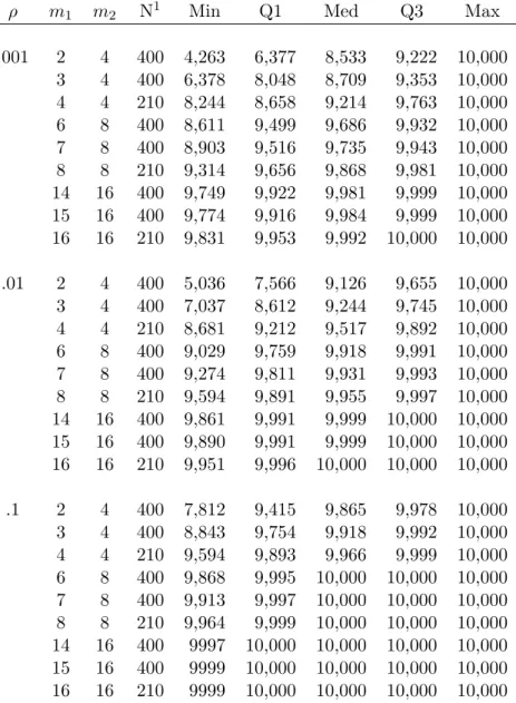
designs. Davies [4] algorithm did not converge for many of the m1 = 2, m2 = 2 cases, so this

combination of number of clusters per treatment group was omitted.

A full factorial combination of these parameters yields 41,472 cases of imbalance. Many of

these lead to the same design with respect to type I error computation. For example, a case

with m1 =m2 = 4, n1 = n2 = 8, r1 = 1 and r2 = 2 will have the same type I error as a case

withr1 andr2 reversed. Unique cases can be characterized as those which have (m1 < m2), or

(m1=m2 andn1 < n2), or (m1 =m2,n1=n2, and r1≤r2). Of the 41,472 cases, 20,880 are unique. Type I error was computed only for unique cases.

(38)

2.4.4 Generation of Cluster Sizes

Cluster sizes were selected from a Gaussian distribution with mean nh, the specified

average cluster size for treatment group h; the standard deviation of the Gaussian

distri-bution was computed as follows. Define nh,max and nh,min as the maximum and

min-imum cluster sizes, respectively, in treatment group h. Since the Gaussian distribution is

symmetric, nh = (nh,max+nh,min)/2. By definition of the enumeration study parameters,

nh,max=rhnh,min. Substituting this back into the previous expression and solving fornh,max

and nh,min yields nh,min= 2h/(rh+ 1) and nh,max= 2hrh/(rh+ 1). Since≈95% percent of

the Gaussian distribution in within two standard deviations of the mean, we fixed nh,min and

nh,max at two standard deviations from mean, so that the standard deviation, σ, can then be

calculated asσ = (nh,max−nh,min)/4 = 2h(rh−1)/4 (rh+ 1). Thus, cluster sizes were given

the distribution:

nhi∼ N n

nh, [2hrh/(rh+ 1)]2

o

.

Define c2 = Prob{(Z <−2)}, where Z ∼ N(0,1). Cluster sizes {nhi} were then computed

such that:

nhi=Z−1[c2+ (i−1) (1−c2)/mh]σ+nh

forh= 1,2 andi= 1, . . . , mh, whereZ−1(p) denotes a function with returns the p-th quantile

from a standard normal distribution. Cluster sizes were not rounded so that actual ratios for

maximum to minimum cluster size were achieved.

2.5 Results of Enumeration Study

2.5.1 Overview

The purpose of this enumeration study is to evaluate which values of each of number of

clusters per treatment group, number of observations per cluster, ratio of maximum to minimum

cluster size, and within-cluster correlation affect Type I error from nominal levels. For the

discussion that follows, we define type I error,α, to be approximately unbiased if it varies from

0.05 by less than a multiplicative factor of 2; that is, if 0.025≤α≤0.1.

Discussion of these enumeration results is complicated as this study enumerated Type I error

(39)

of the parameters of imbalance, so summarization over imbalance factors or combinations of

factors yields at best only general conclusions.

2.5.2 Main Effects of Imbalance Parameters

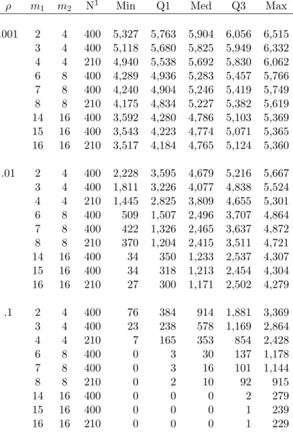
Tables 2.2 - 2.4 give descriptive statistics for type I error over all cases and for the main

effects of each parameter of imbalance and ratios of them, where applicable. No one parameter

of imbalance by itself was a major predictor of type I error, so only few conclusions may be

drawn from displays of type I error for the main effect of each imbalance parameter.

2.5.2.1 Within Cluster Correlation

Section 2 of Table 2.2 displays type I error by ρ, where ρ ∈ {.001, .01, .1}. Regardless of

the imbalance in number of clusters or cluster sizes, the analysis of means weighted by cluster

size was approximately unbiased when ρ=.001. Though sometimes still biased, the analysis

of unweighted means was approximately unbiased for many more cases than the analysis with

cluster size weights when ρ=.1.

Asρ increased, type I error for the analysis of means weighted by cluster size became more

biased. For the analysis of unweighted means, as ρ increased, type I error became less biased,

so that the two weighting schemes show opposite relationships between type I error and ρ.

2.5.2.2 Number of Clusters Per Treatment Group

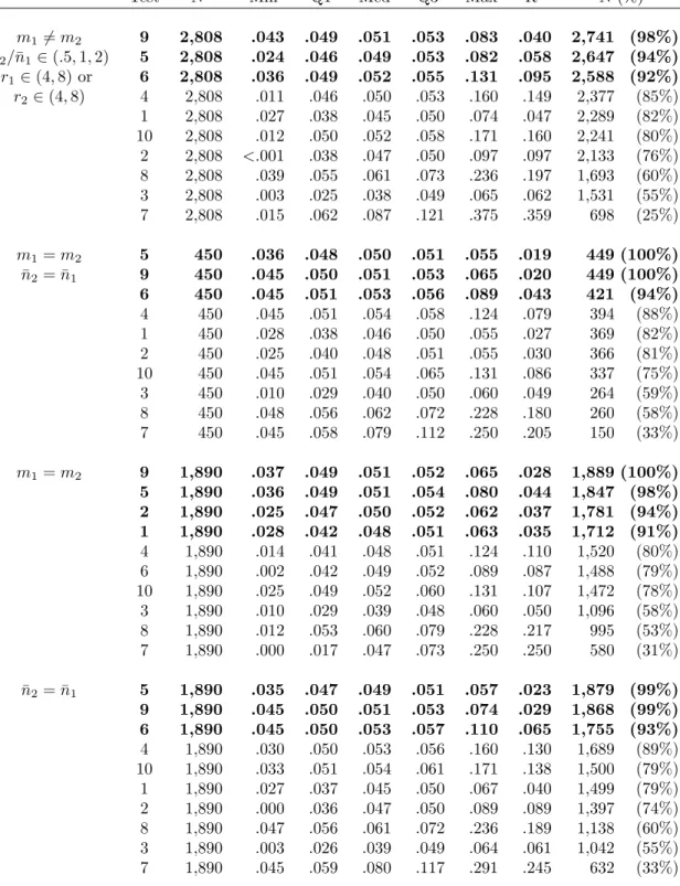
Sections 3-6 of Table 2.2 display type I error for combinations of m1×m2 and their ratio,

m2/m1, where m1, m2 ∈ {2, 4, 8, 16, 32}. Descriptive statistics are similar for combinations

ofm1×m2 with the same ratio, so combinations ofm1×m2 are displayed in order ofm2/m1.

When m1 = m2, that is, when the number of clusters per treatment group is equal, the

analysis of unweighted means provided approximately unbiased type I error regardless of ρ or

imbalance in cluster sizes. No other combinations or ratios of number of clusters uniformly

lead to approximately unbiased type I error in the analysis of unweighted means, nor did any

combinations or ratios of number of clusters do so for the analysis of means weighted by cluster

size.

In general, as m2/m1 increased, type I error became more biased for both weightings. As