THE STRATIFIED OCEAN MODEL WITH ADAPTIVE REFINEMENT (SOMAR)
Edward Santilli
A dissertation submitted to the faculty at the University of North Carolina at Chapel Hill in partial fulfillment of the requirements for the degree of Doctor of Philosophy in the Department of Physics.
Chapel Hill 2015
ABSTRACT
Edward Santilli: The Stratified Ocean Model with Adaptive Refinement (SOMAR) (Under the direction of Alberto Scotti)
ACKNOWLEDGEMENTS
This work was supported by the ONR under grants N00014-05-1-0361 and N00014-09-1-0288 and by the NSF under grants OCE-0825997 and OCE-0729636. Computer resources were provided by the Information Technology Services Research Computing group.
I would like to personally thank Sutanu Sarkar, Vamsi Chalamalla, Masoud Jalali, and Narsimha Rapaka of the UCSD School of Engineering for their correspondence and valuable insight throughout the develop-ment and testing of SOMAR.
TABLE OF CONTENTS
LIST OF TABLES . . . viii
LIST OF FIGURES . . . ix
LIST OF ABBREVIATIONS AND SYMBOLS . . . xii
1 Introduction . . . 1
1.1 Motivation . . . 1
1.2 Equations of Motion . . . 3
1.2.1 The continuum hypothesis . . . 3
1.2.2 The Navier-Stokes Equations . . . 4
1.2.3 The Incompressibility Condition . . . 7
1.2.4 The Hydrostatic Pressure . . . 8
1.2.5 The Boussinesq Approximation . . . 9
1.2.6 The Coriolis Effect . . . 11
1.2.7 Non-Orthogonal Coordinate Systems . . . 13
1.3 Physics Of A Stratified Fluid . . . 15
1.3.1 Buoyancy Oscillations . . . 15
1.3.2 The Internal Wave Equation . . . 16
1.3.3 Dispersion . . . 17
2 Finite Volume Discretization in Curvilinear Coordinates . . . 23
2.1 Freestream preserving metric discretization . . . 24
2.2 Divergence . . . 29
2.3 Gradient . . . 31
2.5 The discrete Hodge-Helmholtz decomposition . . . 34
2.6 Curl . . . 36
3 The Leptic Iterative Method . . . 37
3.1 Introduction . . . 37
3.2 Derivation . . . 40
3.2.1 The desired form of the expansion . . . 41
3.2.2 Summary of the expansion . . . 46
3.2.3 Eliminating horizontal stages . . . 46
3.2.4 An interpretation ofε . . . 48
3.3 Convergence estimates . . . 49
3.3.1 Restricted case . . . 49
3.3.2 General case . . . 52
3.3.3 The leptic solver as a preconditioner . . . 52
3.4 Demonstrations . . . 57
3.4.1 High leptic ratio - Cartesian coordinates . . . 57
3.4.2 Borderline cases - Cartesian coordinates . . . 57
3.4.3 High leptic ratio - Mapped coordinates . . . 60
3.4.4 Borderline case - Mapped coordinates . . . 64
3.5 Discussion . . . 65
4 Time marching schemes . . . 67
4.1 The piecewise-parabolic method for low-Mach flows . . . 67
4.2 Single-level update with ¯b(z)≡0 . . . 68
4.2.1 Unsplit numerical algorithm . . . 69
4.3 Single-level update with ¯b(z)6≡0 and Coriolis effects . . . 72
4.3.1 Derivation . . . 72
4.3.3 The stability of the semi-implicit update . . . 76
4.4 Multi-level update . . . 78
4.5 Solving elliptic equations with AMR and anisotropy . . . 79
4.5.1 Case: λ1 – Krylov methods with semicoarsening . . . 79
4.5.2 Case: λ >1 – The leptic iterative method . . . 80
4.5.3 Case: λ.1 – The leptic preconditioner . . . 83
5 Test Cases . . . 85
5.1 Lock exchange . . . 85
5.1.1 2D flow: Speed of the wave front . . . 85
5.1.2 3D, no-slip flow: The lobe-and-cleft instability . . . 86
5.2 Beam generation . . . 88
5.3 DJL solution . . . 91
5.3.1 2D, solitary wave propagation . . . 92
5.3.2 3D, solitary wave propagation . . . 93
6 Summary and Future Work . . . 98
LIST OF TABLES
1.1 Three-dimensional nonhydrostatic studies . . . 2
2.1 The locations of various geometric quantities in a grid cell . . . 27
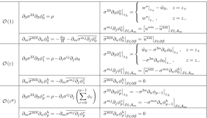
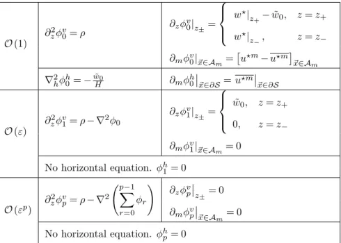
3.1 The leptic expansion in general curvilinear coordinates . . . 47
3.2 The leptic expansion in Cartesian coordinates . . . 48
5.1 Parameters for lab-scale internal wave demonstration . . . 90
LIST OF FIGURES
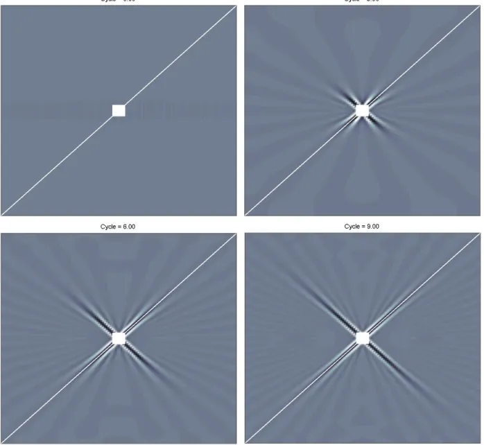
1.1 A simulated shadowgraph of St. Andrew’s Cross, illustrating the direction of each wave’s group velocity. Each slide represents the start of a forcing period (cycle). The solid white square indicates the location of the bobber and the diagonal white line is provided for reference. 20 1.2 A simulated shadowgraph of St. Andrew’s Cross, illustrating the direction of each wave’s
phase velocity. Each slide represents a different portion of a single forcing period (cycle). The solid white square indicates the location of the bobber and the diagonal white line is provided for reference. . . 21
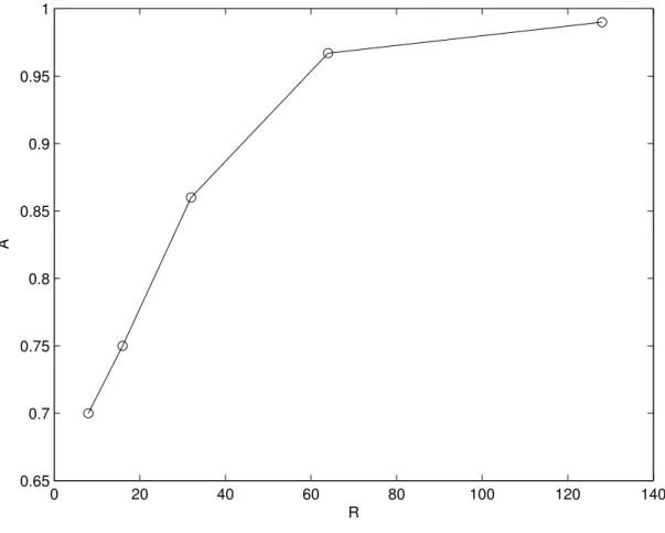
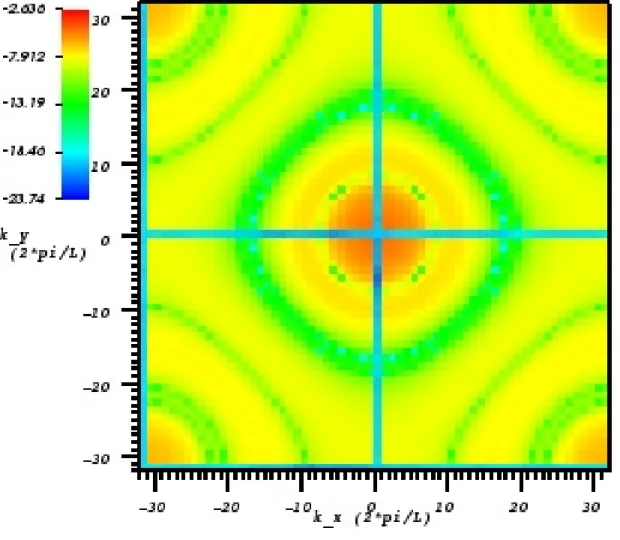
3.1 Attenuation factor as a function of domain aspect ratio for a Poisson problem solved used a standard multigrid scheme. . . 38 3.2 After 26 iterations of BiCGStab, this is a 2-dimensional slice of the residual error’s FFT on
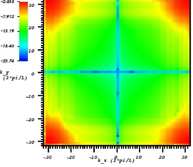
a logarithmic scale. Notice the large error near the center of the plot, indicating BiCGStab’s difficulty eliminating low frequency errors. The vertical and horizontal lines indicating a very low residual (the “crosshairs”) are the zero-frequency modes that must be fixed to agree with the boundary conditions. . . 54 3.3 The residual error after 24 iterations of the leptic solver. This solver eliminates low frequency
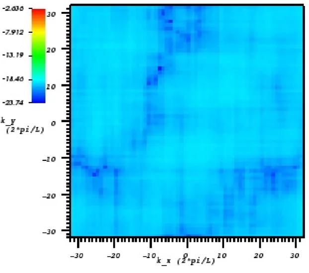
errors much more effectively than high frequency errors, indicating the leptic solver’s potential to serve as a preconditioner for BiCGStab. . . 55 3.4 The residual error of the BiCGStab method when given an initial guess generated by the leptic
solver. . . 56 3.5 Withε≈1/40, the leptic solver is clearly more efficient than BiCGStab. Since we are using
Cartesian coordinates, the leptic solver only needed to perform one horizontal solve. . . 58 3.6 The convergence patterns of the leptic and BiCGStab solvers whenε= 1 and condition number
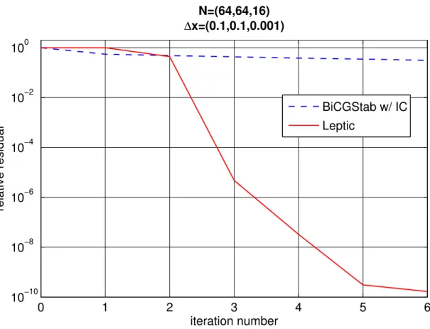
≈105.6. The spikes in the BiCGStab residual are due to restarts. . . . 59 3.7 The performance of various solution methods withε= 1 and condition number≈106.8. After
a few iterations of the leptic solver, BiCGStab can achieve a fast convergence rate. Using a preconditioner such as an incomplete Cholesky decomposition can drive this rate even higher. 60 3.8 Performance of the solvers withε= 4 and condition number≈106.2. The leptic solver began
diverging after it’s third iteration, so control was passed to the Krylov solver. Again, the leptic solver proves most valuable as a preconditioner for the BiCGStab/IC solver whenε=O(1). . 61 3.9 A cross section of the coordinate mapping. The thick line denotes the lower vertical boundary. 62 3.10 Performance of the leptic and Krylov solvers with an anisotropic σij and ε≈0.4. Since
our solver is using Chombo’s matrix-free methods (known asshell matrices in some popular computing libraries such as PETSc [1]), the Cholesky decomposition of the elliptic operator can not be performed. . . 63 3.11 The convergence pattern of a hybrid leptic/Krylov method when ε= 4 on an anisotropic
4.1 A diagram of one complete time step with subcycling. . . 78 4.2 An example of a 2D AMR grid hierarchy. We restrict ourselves to 2D only to simplify the
vi-sualization of the grid hierarchy. In practice, these ideas are used to solve 3D (nonhydrostatic) Poisson problems. The grid scales, ∆ξ, have been nondimensionalized and are provided to exhibit the grid anisotropy. . . 81 4.3 Restriction pattern of a V-cycle when performing a Poisson solve only on AMR level 1. . . . 81 4.4 Restriction pattern of a V-cycle when performing a Poisson solve over AMR levels 0 through
2. We begin with relaxation at AMR level 2, MG depth 0. We then develop corrections iteratively through the coarser grids, eventually using BiCGStab on the coarsest grid at AMR level 0, MG depth 2. We then refine and relax the corrections back up to the finest grid, completing the V-cycle. The shadows of figure 4.2 have been reproduced to provide reference. 82
5.1 Buoyancy contours of a two-dimensional lock-exchange flows. All length and time units are non-dimensionalized for comparison with H¨artel,et. al. [2, 3]. . . 86 5.2 The lobe and cleft instability. Both images were taken from a no-slip run withGr= 1.5×10⁶
andSc= 0.71 at t=11.36. . . 87 5.3 Diagram of beam generation problem setup (not drawn to scale). The background buoyancy
increases linearly with depth at a rate−d¯b/dz=N2 for all runs. . . 89 5.4 Large-scale calculation at a model ridge with critical slope at Ex = 0.066. The color plots
represent the streamwise velocity field showing internal wave beams. In the left panel, the computational grid is superimposed to emphasize the higher resolution near the topographic relief and the beams after adaptive mesh refinement. The right panel shows the steep, near-bottom isopycnals. . . 89 5.5 A comparison of the internal wave beam using three solution methods. The profiles shown
are the root-mean-square, horizontal, baroclinic velocity sections atx/l=−1 over the seventh tidal cycle. . . 91 5.6 The solution to the DJL equation propagating in a long, thin channel. The thick black line
traces the median isopycnal and the color plot depicts log(KE), where the energy has been normalized by its maximum value at t= 0. The top panel illustrates the initial waveform. The bottom panel shows that after 200 seconds, the waveform has travelled approximately 90 channel heights, but only a trace amount of energy (colors on the blue end of the spectrum are less thanO(10−3)) has leaked from the trailing end. . . . . 94 5.7 An overhead view of the 3D solitary wave’s evolution. Each panel is a horizontal slice through
LIST OF ABBREVIATIONS AND SYMBOLS
AMR Adaptive Mesh Refinement
BiCGStab Stabilized Bi-Conjugate Gradient Method CPU Central Processing Unit
DNS Direct Numerical Simulation GCM Global Circulation Model GFD Geophysical Fluid Dynamics
KdV Korteweg-de Vries
LES Large Eddy Simulation
LHS Left-Hand Side
MG Multigrid
MITgcm Massachussetts Institute of Technology General Circulation Model MPI Message Passing Interface
NLIW Nonlinear Internal Wave
NSE Navier-Stokes Equations
PDE Partial Differential Equation
PETSc Portable, Extensible Toolkit for Scientific Computation PPM Piecewise Parabolic Method
RHS Right-Hand Side
RMS Root-Mean-Square
ROMS Regional Ocean Modeling System
SUNTANS The Stanford Unstructured-Grid, Nonhydrostatic, Parallel Coastal Ocean Model UNC University of North Carolina
bT The total buoyancy (reduced gravity)
¯b The background buoyancy profile (This is a function of zalone.)
b The buoyancy deviation
w Vertical Cartesian velocity component
ui Curvilinear component of the 3-dimensional vector ~u un,i ui at timetn(nwill never be used as an index.) u?,i An unprojected velocity component
uiAD The time and face centered, projected advecting velocity uiH Interpolation of uiAD to all cell faces
ν,κ Kinematic viscosity and scalar diffusion parameters {x,y,z}or {xα} Cartesian coordinates
{ξ,η,ζ}or{ξi} General curvilinear coordinates gij,gij The metric tensor and its inverse
J The Jacobian determinant
CC Cell centered.
FC Face centered.
MAC Marker-and-cell scheme that describes the exact, discrete projection method φ Scalar used during the MAC projection
πl Pressure computed during the level l, CC velocity projection AvCC→FC Averaging operator that sends CC data to FC data
AvFC→CC Averaging operator that sends FC data to CC data
Average rate of dissipation of turbulence kinetic energy per unit mass ijk The totally anti-symmetric permutation symbol
CHAPTER 1: Introduction
Section 1.1: Motivation
The numerical simulation of geophysical and astrophysical flows presents several challenges. One major difficulty is that the flows are often characterized by a marked anisotropy due to a combination of geometrical and dynamical constraints. In geophysical flows, geometrical constraints cause the horizontal scales to be much larger than the vertical scale, while dynamical constraints, such as gravity, rotation, and magnetism if the fluid is conducting, introduce a preferred direction, which severely constrains the flow at very large scales [4, 5, 6]. In the following, we will concentrate on oceanic applications, though the techniques presented in this manuscript could also be applied to atmospheric and, to a lesser extent, astrophysical flows. In the ocean, temporal scales range from the millennial time scale of the Meridional Overturning Circulation [7] to seconds in the case of small scale turbulence [8], though the type of processes for which we are developing the model discussed in this manuscript span the smaller range from days (internal tides) to seconds (turbulence). Clearly, a unified modeling framework is out of reach for the foreseeable future. Rather, a set of tools has emerged since the pioneering work of Bryan in the late 1960’s [9]. By the early 2000s, a well established suite of models existed covering either the very large scales or the very small scales. For the case of large scales, provided the horizontal scale of the motion remains much larger than the local depth, the pressure is found to satisfy to leading order the hydrostatic approximation. This greatly simplifies the equations, and around this core approximation a number of General Circulation Models (GCMs) have been developed differing among themselves based on the choice of dependent and independent variables, the type of discretization, and so on. For more details, and also for a historical perspective, the reader is referred to Haidvogel and Beckmann [6]. Due to the nonlinear nature of the underlying dynamics, the unresolved scales do have a nontrivial effect on the resolved scales. Their effect is usually included with parameterization schemes which range in complexity from simple constant “eddy” viscosity and diffusion, to more sophisticated closure schemes [10]. At the opposite end of much smaller scales, the hydrostatic approximation obviously breaks down, but the flow is also much less anisotropic and rotation is negligible. This dynamical regime can be efficiently dealt with Direct Numerical Simulation (DNS) and Large Eddy Simulation (LES) [11, 12], which developed rather independently and parallel to the development of the large scale GCMs.
Study site Code Lepticity Reference
South China Sea SUNTANS 7 Zhang,et. al. [16] Monterey Bay SUNTANS >4 Kang,et. al. [17] Monterey Bay SUNTANS >14 Jachec,et. al. [18] Luzon Strait MITgcm 3.1 Guo,et. al. [19] Andaman Sea MITgcm 3.3 Vlasenko,et. al. [20] Gibraltar Strait MITgcm 0.7 Vlasenko,et. al. [21] Cayuga Lake MITgcm 1.2 Dorostkar,et. al. [22]
Table 1.1: Three-dimensional nonhydrostatic simulations. The Monterey Bay simulations where not designed with NLIWs in mind, but are included as they include the effect of complex topography on internal waves. To properly account for the physical (as opposed to numerical) sources of dispersion in the propagation of NLIWs, the grid lepticity must be less than one. Vitousek and Fringer [23] define the lepticity as the ratio of the horizontal grid spacing to the depth of the internal interface. Table adapted from Dorostkar [22].
phenomena are usually highly localized, and in an appropriate sense not far from being hydrostatic (though the departure is essential to their dynamics). Improvement on the current status thus revolves in developing a framework that takes advantage of these properties to effectively manage the numerical resources and improve the convergence rate of the iterative solver in high aspect ratio conditions.
A description of such framework is the object of the remainder of this thesis. It combines the flexibility of Adaptive Mesh Refinement (AMR) [24] to effectively husband finite numerical resources with the Leptic Poisson Solver [25] to bring the convergence rate of the Poisson solver within acceptable limits.
Section 1.2: Equations of Motion
Before we delve into numerical algorithms, it is worthwhile to define the equations of motion that we wish to solve. A description will be presented in terms of the underlying physical principles, accounting for and justifying the approximations we use along the way.
1.2.1: The continuum hypothesis
The smallest length scales of dynamical importance in a fluid are the Kolmogorov scale, where molecular viscosity converts kinetic energy into heat, and the Batchelor scale, where diffusive time scales rival inertial time scales [26]. In the ocean, these scales can be as small as O(1mm) [27, Sec. 2.2]. Far smaller, is the mean-free-path of the individual molecules of the fluid, which at standard temperature and pressure is less than O(1nm) [28, Sec. 1.2.1]. With 6 orders of magnitude between these scales, we can, to a great degree of accuracy, ignore the molecular structure of the ocean. In doing so, we assume that the fluid is a continuum rather than a collection of discrete particles. This continuum hypothesis enables us to convert integral formulations of the dynamics into differential formulations. In this section, we will methodically derive the differential equations of motion that contain the physics of our ocean model.
1.2.2: The Navier-Stokes Equations
Strictly speaking, the Navier-Stokes equations are a system of equations that dictate the evolution of momentum for a fluid whose stresses can be expressed as−gijP+µ(∇iuj+∇jui) +λgij∇ ·~u, where µand λ parameterize the stresses due to shear and compression of a fluid parcel [29, Sec. 38]. When dealing with a stratified fluid, the momentum equation is joined with an evolution equation for density as well. For our purposes, the Navier-Stokes equations will refer to the complete system of equations that are solved to determine the state of the fluid. In this section, we will therefore derive both a mass transport equation and a momentum conservation law. In subsequent sections, we will focus on applying and justifying approximations that tailor the Navier-Stokes equations to our stratified oceanic needs.
Conservation of Mass
We begin by defining the mass of a fluid parcel, V(t), in terms of the fluid’s density field,
m=
Z
V(t)
ρ(~x, t)dV. (1.1)
In general, the total mass of a fluid need not be conserved. In the ocean, sunlight penetrates approximately 200 meters into the surface, changing the chemical and biological makeup of the fluid [30, 31]. Evaporation and precipitation, which tend to be locally out of balance, can add or remove mass to the surface, resulting in horizontal displacements of fluid to restore balance with the atmospheric pressure [32, Sec. 9.9, 9.14, 11.14]. Additionally, evaporation plays a significant role in removing heat energy and increasing salt concentrations at the ocean’s surface [32, Sec. 2.6, 2.7]. For our purposes, we will assume that the mass inside the domain is, in fact, conserved and that any mediating factors can be handled by an appropriate equation of state or through a judicious choice of boundary conditions. To conserve total mass, we can fix the parcel boundary in time and assume that any change in local mass can only arise through a mass flux though the boundary ∂V(t0). That is,
Z
V(t0)
∂ρ(~x, t)
∂t dV =−
I
∂V(t0)
[~u(~x, t)ρ(~x, t)]·d ~A (1.2a)
=−
Z
V(t0)
∇ ·[~u(~x, t)ρ(~x, t)]dV, (1.2b)
where we used Gauss’ law and defined~u(~x, t) is the velocity of the fluid at each point in the domain. Since V(t0) is arbitrary, we can equate the integrands to obtain the differential form of our conservation law,
This formula describes the kinematics of the density field imposed by a physical conservation of mass. It should be pointed out that since eq. 1.2 came from setting the time derivative of eq. 1.1 to zero, we have the geometric identity
dQ(t) dt = d dt Z V(t)
q(~x, t)dV =
Z
V(t)
∂q(~x, t)
∂t +∇ ·[~u(~x, t)q(~x, t)]
dV, (1.4)
which applies to any scalar, Q(t), and its associated density, q(~x, t), over any volume V(t) at any timet. Although this identity is simply a multi-dimensional version of the Leibniz integal rule [33], it has been given several names throughout the literature and has several distinct derivations. In many derivations, including one put forth by Osbourne Reynolds [34], the boundary,∂V(t), deforms in such a way as to keepQconstant. In that case, the velocity field,~u(~x, t), is not only interpreted as the fluid velocity, but also as a vector that describes this deformation of the boundary. The so-called Reynold’s Transport Theorem, eq. 1.4, is in fact a very general geometric identity that is applicable to any scalar and its associated density and is independent of the choice and evolution ofV(t).
As an interesting note, we could have arrived at eq. 1.4 with a bit less effort by computing the time derivative ofQ(t) with a Lie derivative applied to the formq(~x, t)dV [35, Sec. 4.3]. However, this technology was not available in Reynolds’ time, and currently, the machinery of exterior differential forms has not yet reached widespread use.
Conservation of Momentum
To conserve momentum, we tally all of the forces acting on a fluid parcel and apply Newton’s second law. We split the forces into a vector that describes the forces acting on the entire fluid parcel,F~body(~x, t), and a tensor that describes the forces acting on the boundary of a fluid parcel, F↔surf(~x, t). Newton’s second law then takes the form
d dt
Z
V(t)
ρ~u dV =
Z
V(t) ~
FbodydV +
I
∂V(t) ↔
Fsurf·d ~A.
From now on, the function parameters, (~x, t), will not be explicitly identified unless needed for clarity. Also, as is necessary in continuum mechanics, the forces in the intergrands are actually forces per unit volume.
As described in section 1.2.2, we can apply the Reynolds Transport Theorem, eq. 1.4 to the time derivative,
Z
V(t)
∂(ρ~u)
∂t +∇ ·(ρ~u~u)
dV =
Z
V(t) ~
FbodydV +
I
∂V(t) ↔
By expanding the derivatives on the LHS and applying the conservation of mass equation 1.3, we get
Z
V(t) ρD~u
DtdV =
Z
V(t) ~
FbodydV +
I
∂V(t) ↔
Fsurf·d ~A,
where thematerial derivative orLagrangian derivative,D/Dt, is a time derivative operator that follows the fluid parcel as it measures the rate of change of a quantity. It is defined by
D Dt =
∂
∂t+~u· ∇.
We will identify the body force with the gravitational force, −ρgˆz, plus a yet unidentified external force, ~
Fext. The gravitational force serves to define the negative vertical direction,−ˆz. Also, we can apply Gauss’ Law to the surface term and, as usual, equate the integrands. This produces a rather general momentum conservation law in its differential form,
ρD~u
Dt =−ρgzˆ+ ~
Fext+∇· ↔ Fsurf.
The surface forces can be split into an isotropic tensor,−P↔1 , and its deviation,↔τ. This casts the equations into the following familiar form,
ρD~u
Dt =−∇P+∇· ↔
τ −ρgˆz+F~ext. (1.5)
As long as the fluid velocities are much smaller than the RMS velocities of the molecular motion, which is true in the ocean to a very high degree, then the fluid remains quasi-static andP can be identified with the thermodynamic pressure [36, Sec. 4.5]. The tensor ↔τ is called thedeviatoric stress tensor. By considering the torques on a fluid parcel, it can be shown that this tensor is symmetric. Also, by requiring Galilean invariance, this tensor cannot depend on the fluid velocity, ~u, directly but can depend on the velocity gradients,∇~u. In general, the relation between ↔τ and∇~ucan be quite complex, however for aNewtonian fluid, the relationship is assumed linear. Furthermore, since pure rotation of a parcel imposes no stress, we can require ↔τ to depend only on the symmetric part of ∇~u, that is,↔S= (∇~u+ (∇~u)T)/2. This symmetric tensor is called thestrain rate tensor and describes the deformation of the fluid parcel [27, Ch. 17].
If the fluid reacts to stresses isotropically, then the fluid itself is said to be isotropic and the relation between the deviatoric stress tensor and the strain rate tensor becomes remarkably simple [36, Sec. 4.5],
↔
This relation has only two parameters that depend on the thermodynamic state, µand λ. Note that this form of ↔τ only depends on the velocity through↔S since∇ ·~u= Tr[↔S].
1.2.3: The Incompressibility Condition
Consider the conservation of mass equation, 1.3. An application of the product rule for derivatives and a bit of algebra casts the law into a different form,
∇ ·~u=−1 ρ
Dρ
Dt. (1.7)
In general, eq. 1.7 will not be zero since the density of a fluid parcel is locked into an equation of state with other thermodynamic quantities. However, if the flow is not turbulent, then the irreversible conversion of kinetic energy into heat is negligible and we can assume the flow is isentropic. In that case, we can consider the density,ρ, the total pressure,P, and the entropy,s, as our thermodynamic triplet and associate changes in density (or volume) of our fluid parcel with changes in pressure alone sinceds= 0 [37, Sec. 2].
For an isentropic flow, the speed of sound in the fluid is given by [37, Sec. 63]
c2=
∂P
∂ρ
s .
This converts eq. 1.7 into
∇ ·~u=− 1 ρc2
DP
Dt
s
. (1.8)
We can now non-dimensionalize this equation via the transformations [36, Sec. 4.11]
x?=x l, t
?=U t l , ~u
?= ~u U, ρ
?= ρ ρ0
, P?=P−Patm ρ0U2
,
wherelandU are length and velocity scales representative of the flow,ρ0 is a density scale representative of the fluid, andPatmis the pressure at the surface of the ocean. The conservation of mass equation 1.8 now becomes
∇?·~u?=−M2 1 ρ?
DP? Dt?
s ,
If we explicitly write out eq. 1.7 in Cartesian coordinates, we see that
∂u ∂x+
∂v ∂y+
∂w
∂z =O(M 2).
So, to approximately one part in a million, the 3 terms of the divergence balance each other. In other words, although each term of the divergence is typically significantly larger than O(M2), these potentially large terms result in a small sum. In the ocean, this means that the horizontal convergence or divergence of fluid is primarily balanced by a net upwelling or downwelling, rather than a density change. Thus, for the low-Mach flows of the ocean, we impose theincompressibility condition,
∇ ·~u= 0. (1.9)
Note that this does not mean that the density of a fluid parcel does not change. It simply expresses the fact that density changes are governed by dynamics that do not significantly effect the convergence or divergence of fluid. The dynamics of the density field are primarily derived from the fluid’s equation of state. In particular, the relation among density and temperature will be discussed in section 1.2.5.
1.2.4: The Hydrostatic Pressure
If we combine eqs. 1.5, 1.6, and 1.9, we get
ρD~u
Dt =−∇P−ρgˆz+∇ ·(µ∇~u) + ~ Fext.
Note that the incompressibility condition simplifies the stress tensor to contain just a single thermodynamic parameter, the molecular viscosity,µ. If we divide both sides by a reference density,ρ0, that is representative of the background stratification1, we obtain
ρ ρ0
D~u Dt =−
1 ρ0
∇P−ρg ρ0 ˆ
z+∇ ·(ν∇~u) + 1 ρ0
~ Fext,
where the new quantity,ν=µ/ρ0, is the kinematic viscosity.
Using the background stratification, ¯ρ(z), and the pressure at the surface of the ocean, Patm, we can define the hydrostatic pressure,
¯
P=Patm+g
Z 0
z ¯ ρ(z0)dz0,
1Reasonable choices ofρ
and perform the following algebraic maneuver,
ρ ρ0
D~u Dt =−
1 ρ0
∇ P−P¯
−(ρ−ρ)g¯ ρ0
ˆ
z+∇ ·(ν∇~u) + 1 ρ0
~ Fext.
We can now define the buoyancy deviation, b, the specific hydrostatic pressure deviation, p, and the specific external force,fext,
b=gρ−ρ¯ ρ0
, p=P− ¯ P ρ0
, f~ext= ~ Fext
ρ0 .
With these definitions, the conservation of momentum equations become
ρ ρ0
D~u
Dt =−∇p−bˆz+∇ ·(ν∇~u) + ~
fext. (1.10)
In the ocean, since the ratio of horizontal to vertical length scales are approximately 1000 : 1, it is often assumed that the horizontal wavenumbers,k, are much smaller than the vertical wavenumbers,m. Through the forthcoming derivation of relation 1.23 in section 1.3.3, it can be seen that in the limitk/m→0, we can approximate Dw/Dtto be zero. This is called the hydrostatic approximation and arises from a geometric constraint on the flow. Dynamically, this approximation applied to the stratified ocean assumes that the flow is very nearly in the plane of the background isopycnals (surfaces of constant density). With the vertical acceleration assumed negligible in the momentum equation 1.10, the only source of diapycnal motion comes from the incompressibility equation 1.9. While many regional and global ocean models assume hydrostasy [13], the work presented in this document will take strides to avoid it. As we shall see, the dynamics of internal waves are non-hydrostatic, but highly localized. Therefore, while the large majority of the ocean is very nearly hydrostatic, there are small, localized patches that are non-hydrostatic. This fact will be of importance in what follows.
1.2.5: The Boussinesq Approximation
If we neglect salinity and assume a linear equation of state,ρ=ρ0[1 +α(T−T0)], then the conservation of momentum equation 1.10 becomes
[1 +α(T−T0)] D~u
Dt =−∇p−bzˆ+∇ ·(ν∇~u) + ~ fext.
Boussinesq approximationon the conservation of momentum equation,
D~u
Dt =−∇p−bˆz+∇ ·(ν∇~u) + ~
fext. (1.11)
Although it is tempting to make a similar simplification to the density field that is buried inside the buoyancy, b, we cannot do so. As stated in section 1.2.4, the majority of the ocean is nearly in hydrostatic balance, which places an exacting importance on the buoyant forcing. Regardless of whether or not the Boussinesq approximation is assumed, the the dynamical forcing terms on the RHS of the z-component of this equation are very nearly in balance throughout the ocean and none of these terms can be removed or simplified [40, Sec. 3.7].
Our linear equation of state has further consequences due to the fact that the temperature of a fluid parcel,T, obeys the heat equation,
DT Dt =κ∇
2T,
where κis the thermal diffusivity of the fluid. Cushman-Roisin and Beckers show that this heat equation is a result of Fourier’s law of heat conduction and the incompressibility condition applied to the first law of thermodynamics [40, Sec. 3.4–3.7]. By applying the material derivative to the linear equation of state, we get
Dρ Dt =ρ0α
DT
Dt =ρ0ακ∇
2T=κ∇2ρ.
That is,
Dρ Dt =κ∇
2ρ. (1.12)
Given the incompressibility condition, eq. 1.9, the Boussinesq approximation invalidates conservation of mass, eq. 1.7, in favor of conservation of volume. In other words, eq. 1.9 still holds, but eq. 1.7 does not. It has been replaced with eq. 1.12 which allows for fictitious mass fluxes to serve as a proxy for thermal diffussion [27, Sec. 2.4.3]. Since sea water is very nearly incompressible, this is a reasonable approximation for much of the dynamics of the ocean. This removes the dynamically unimportant acoustic waves from the model, allowing for a large increase of the maximum stable time step in our numerical integration of the Navier-Stokes equations [41, pp. 335–336]. On the other hand, if we wish to model the fluid’s thermodynamics, we would be at a loss. Assuming the conservation of volume spoils even the most basic thermodynamic principles, such asdW=P dV.
involves buoyancy rather than density. The total buoyancy and background buoyancy are defined via
bT =g ρ−ρ0
ρ0
and ¯b=gρ¯−ρ0 ρ0
(1.13)
which is made consistent with our definition of the buoyancy deviation throughbT = ¯b+b, and we must keep in mind that the background buoyancy profile is a function of z alone. In terms of the total buoyancy, the equation of state readsbT =α(T−T0) and eq. 1.12 becomes
DbT Dt =κ∇
2b T.
While we do wish to diffuse the dynamic buoyancy deviation, b, we do not wish to do the same to the background buoyancy, ¯b, since this profile is often maintained by unmodeled phenomena. To this end, we manually remove the term that diffuses the background buoyancy, leaving
Db Dt+w
∂¯b ∂z =κ∇
2b. (1.14)
If the background stratification is stable, then heavy fluid lies beneath lighter fluid and d¯b/dz <0. To emphasize this, we defineN= (−d¯b/dz)1/2 and cast the buoyancy evolution equation into its final form,
Db Dt=N
2w+κ∇2b. (1.15)
1.2.6: The Coriolis Effect
In Geophysical Fluid Dynamics (GFD), it is customary to denote the local eastward, northward, and upward unit vectors as ˆx, ˆy, and ˆz, respectively [40, Sec. 2.5]. If we take the time derivative of any vector,
~
Q, in this rotating basis, then we must account for the explicit time dependence ofQ~ in the rotating frame and the change in the basis vectors’ orientation. Both of these terms are neatly derived and packaged in a formula from Marion and Thornton [42, p. 390]
d ~Q dt
!
fixed
= d ~Q dt
!
rotating
+~Ω×Q,~
velocity as measured by an inertial observer and an observer on the surface of the rotating Earth,
~
ufixed=~urotating+Ω~×~x.
We can now differentiate again to obtain an acceleration as measured by an inertial observer,
~afixed=
d
dt
fixed ~ ufixed
=
d dt
fixed
h
~
urotating+~Ω×~x
i
=
"
d dt
rotating +Ω×~
# h
~
urotating+Ω~×~x
i
=~arotating+ 2~Ω×~urotating+~Ω×Ω~×~x.
The 2Ω~×~urotating term is the Coriolis acceleration term. The Ω~×Ω~×~xterm is a centrifugal acceleration term and can be reduced to−Ω2Rcos(Θ)ˆz, whereRis the fluid parcel’s distance to the center of the Earth and Θ is the local latitude. Since the centrigugal acceleration is oriented downward, we simply redefine the local gravitational acceleration constant, g−Ω2Rcos(Θ)→g, and neglect the explicit addition of this term in the dynamical equations. At 45◦ N latitude, this redefinition alters the value ofgby approximately 0.2%. Alternatively, if we express the centrifugal acceleration as the gradient of a potential by assuming cos(Θ) is uniform throughout the domain of interest, we can simply push the entire forcing term into the yet undetermined pressure.
Our momentum equation 1.11, can now be expressed in the Earth’s rotating frame by the addition of a Coriolis term,
D~u Dt+ 2
~
Ω×~u=−∇p−bˆz+∇ ·(ν∇~u) +f~ext. (1.16)
In the ocean, the vertical velocity,w, is typically much smaller than the horizontal velocities,uand v, due to geometric considerations. This simplifies the Coriolis term in the momentum equation since
2~Ω×~u= 2 Ω[(wcos Θ−vsin Θ)ˆx+usin Θˆy−ucos Θˆz] ≈2 Ω[−vsin Θˆx+usin Θˆy−ucos Θˆz]
=−f vx+ˆ f uˆy−2 Ω cos Θuˆz,
to regions of the ocean in which the latitude does not vary much. In those cases, we employ the f-plane approximation by assuming that the Coriolis parameter is uniform throughout the domain of interest. As a final simplification, the z-component of the Coriolis acceleration, −2 Ω cos Θu, is often assumed negligible compared to the pressure gradient term, leaving
2~Ω×~u≈ −f vˆx+f uˆy.
For a complete description of the scales of oceanic motion and the simplification of the Coriolis terms, see Cushman-Roisin and Beckers [40, Sec. 4.3].
1.2.7: Non-Orthogonal Coordinate Systems
Equations 1.16, 1.15, and 1.9 constitute the Incompressible Navier-Stokes equations under the Boussinesq approximation,
D~u Dt+ 2
~
Ω×~u=−∇p−bˆz+∇ ·(ν∇~u) +f~ext (1.17a) Db
Dt =N
2w+κ∇2b (1.17b)
∇ ·~u= 0 (1.17c)
We wish to formulate eqs. 1.17 in general curvilinear coordinates without the use of Christoffel symbols since in 3D, they are 18 independent functions that are expensive to compute and store.
To proceed, we will use index notation and sum over repeated indices. Greek indices will refer to Cartesian components of vectors and tensors, while latin indices will refer to curvilinear components. {xα} are the Cartesian coordinates and{ξi}are the curvilinear coordinates. The metric tensor is defined via the Jacobian elements,
gij=
X
α ∂xα
∂ξi ∂xα ∂ξj ,
the inverse metric tensor is denotedgij, and the Jacobian determinant is J =pdet(gij). The generalized gradient and divergence operators are
∇if=gij∂jf and ∇iui= 1 J∂iJ u
j, (1.18)
generalized by contracting the covariant divergence and covariant gradient operators. When operating on a scalar, the Laplacian is expressed as
∇2= 1 J∂iJ g
ij∂ j.
When applied to the curvilinear components of a vector or tensor, this operator becomes more complicated and involves Christoffel symbols. For this reason, we will always apply the Laplacian to scalars and Cartesian components of vectors and tensors. For a complete description of the notation used here and a thorough explanation of Riemannian geometry, see Lovelock and Rund [43].
The incompressibility condition is generalized by applying the covariant divergence of eqs. 1.18 to the curvilinear velocity components,
∂iJ ui= 0,
where we have multiplied both sides byJ to simplify the equation. The buoyancy equation can be converted similarly,
∂b ∂t+u
i∂
ib=N2w+κ∇2b, where the advection term utilizes the convenient transformation
uβ ∂ ∂xβ =u
i∂ i.
The same simple transformation could have been applied to the advective term involving the background buoyancy, but since the ¯bprofile is not dynamic, and it is a function of zalone, it is convenient to compute this term in Cartesian coordinates. To finalize the covariant buoyancy equation, we cast the advective term into a conservative form by use of the incompressibility condition. The resulting form,
∂b ∂t+
1 J∂iJ u
ib=N2w+κ∇2b,
is better suited to the numerical schemes that will be presented in chapter 4.
To generalize the momentum equation, we will again convert the derivative operators using eqs. 1.18, but we will apply them to the Cartesian components of the velocity vector to avoid Christoffel symbols. These updated components can then be used to generate the curvilinear velocity vector viaui=uα(∂ξi/∂xα) if needed. Theα-component of the momentum equation becomes
∂uα ∂t +u
i∂
Note that with ν removed from the Laplacian, we are assuming a uniform viscosity. Also note that, by definition, gαi= (∂ξα/∂xj)gji. As in the buoyancy equation, we wish to cast the advective term into a conservative form. The resulting set of equations is
∂uα ∂t +
1 J∂iJ u
iuα+ 2εα
ijΩiuj=−gαi∂ip−bˆzα+ν∇2uα+fextα (1.20a) ∂b
∂t+ 1 J∂iJ u
ib=N2w+κ∇2b (1.20b)
∂iJ ui= 0. (1.20c)
Thef-plane approximation is recovered by replacing 2εα
ijΩiuj withf εαij ∂ξi
∂zuj.
Section 1.3: Physics Of A Stratified Fluid
1.3.1: Buoyancy Oscillations
Consider a fluid parcel removed vertically a small distance δz from its hydrostatic position, z0. The parcel then has a buoyancy of ¯b(z0) and is surrounded by fluid whose buoyancy is ¯b(z0+δz). If we choose ρ0= ¯ρ(z0), then, by definition,
¯
b(z0) =g ¯
ρ(z0)−ρ0 ρ0
= 0.
We can use this in a Taylor expansion of ¯b(z0+δz),
¯
b(z0+δz) =δz d¯b dz
z
0
+O δz2.
If the fluid is stably stratified, thend¯b/dz <0. To emphasize this, we will define
N2=−d¯b dz
z0
.
Now, by construction, our fluid parcel of zero buoyancy has navigated into a region whose ambient buoyancy is approximately−N2δz. Newton’s second law provides an equation of motion for the displaced parcel,
d2δz dt2 =−N
2δz.
δz∼e±iN twithN a real-valued angular frequency of the motion called theBrunt-V¨ais¨al¨a frequency. These
buoyancy oscillations are at the heart of internal wave modeling. As we will see in section 1.3.3, this simple harmonic motion provides the smallest timescale of dynamical importance in laminar regimes of a stratified ocean.
1.3.2: The Internal Wave Equation
Buoyancy oscillations occur when a stably stratified fluid is perturbed from its rest hydrostatic state. Consider a continuously stratified fluid whose rest state is characterized by~u= 0,ρ= ¯ρ, andP= ¯P. As usual, ¯
ρ is the background density profile and ¯P is its associated hydrostatic pressure defined by∂P /∂z¯ =−¯ρg. Deviations from this rest state are described in Cartesian coordinates under the Boussinesq approximation by eqs. 1.17. If we ignore viscous, diffusive, and nonlinear effects, these equations become
∂u
∂t −f v=− ∂p
∂x (1.21a)
∂v
∂t+f u=− ∂p
∂y (1.21b)
χ∂w ∂t =−
∂p
∂z−b (1.21c)
∂b ∂t=N
2w (1.21d)
∂u ∂x+
∂v ∂y+
∂w
∂z = 0, (1.21e)
whereχ is set to 1 for non-hydrostatic flows and 0 for hydrostatic flows.
Buoyancy oscillations can be recovered by considering the particular non-hydrostatic solutions with u= v=∂p/∂z= 0. These solutions must satisfy
∂w ∂z = 0 ∂2w
∂t2 +N 2w= 0 ∂2b
∂t2+N 2b= 0.
Of significant importance is the fact that both p and w are constant throughout vertical water columns. This fact will crop up again when considering how our adaptive grids will be structured in the vicinity of an interfacial wave (eg. a depression in the pycnocline).
equations, then add to obtain ∂ ∂t ∂u ∂x+ ∂v ∂y =f ∂v ∂x− ∂u ∂y
− ∇2hp.
Application of the incompressibility condition produces
−∂ ∂t
∂w ∂z =f
∂v
∂x− ∂u ∂y
− ∇2 hp.
We must now return to equations 1.21 to produce a vorticity equation. Applying derivatives and subtracting yields ∂ ∂t ∂v ∂x− ∂u ∂y
=f∂w ∂z. These equations can be combined to eliminate the vorticity
∂2 ∂t2+f
2 ∂w ∂z = ∂ ∂t∇ 2 hp.
Finally, we can apply ∂/∂z and substitute the z-component of the linearized momentum equation and linearized buoyancy equation to arrive at a Sobolev equation [44], called theinternal wave equation,
χ∇2h+ ∂ 2
∂z2
∂2w ∂t2 +
N2∇2h+f2 ∂ 2
∂z2
w= 0. (1.22)
1.3.3: Dispersion
Equation 1.22 is a hyperbolic linear PDE, which means we can expect traveling solutions of the form ei(K~·~x−ωt). In this section, we will restrict ourselves to two spatial dimensions without loss of generality. Upon substitution into eq. 1.22, we find thedispersion relationamong the temporal frequencies, ω, and the spatial frequencies,K~ = (k, m),
ω2=N
2k2+f2m2
χk2+m2 . (1.23)
Non-hydrostatic case (χ= 1)
If we define αto be the angle between the vertical and the direction of phase propagation, ˆK, then this relation is simply expressed as
ω=±Nsinα. (1.24)
Therefore, given a particular stratification,N, and a particular forcing frequency,ω, all internal waves will have lines of constant phase that propagate at angles of±αwith the vertical. Furthermore, since sinα≤1, the forcing frequency must be less than or equal to the frequency of buoyancy oscillations, N, if internal waves are to form. If ω > N, the energy given to the system will disturb the fluid locally and produce turbulence, but the energy will not be carried away by waves [40, Sec. 13.2]. Thus, the Brunt-V¨ais¨al¨a frequency represents the highest frequency of wave-like motion in the ocean.
Given a dispersion relation, we can gather useful information about the speeds of the Fourier modes that construct the internal waves. The phase speed in thex-direction is given by following a portion of the wave that is at constant phase, φ0, along thex-axis. That is, given the phase function, φ(~x, t) =K~ ·~x−ωt, we can choose a particular value, φ(~x, t) =φ0, and measure the position of this phase value as it moves along thex-axis. This producesφ0=kx−ωt, orx(t) = (ω/k)t−φ0/k. The phase speed along thex-axis is simply the coefficient oft. When we perform the same analysis along the z-axis and along the direction of phase propagation, ˆK, we recover the following formulas
c(x)p = ω k, c
(z) p =
ω
m, cp= ω K.
It is extremely important to notice thatc(x)p andc(z)p are not thexandz components of the phase velocity, cpK. This fact is emphasized in the limit of purely horizontal wave motion,ˆ α→ ±90◦. If we letk→K and m→0, thenc(x)p →cpwhilec(z)p → ±∞.
Using our dispersion relation, eq. 1.24, we find the phase speeds for internal waves,
c(x)p =± N K, c
(z) p =±
N
Ktanα, cp=± N Ksinα.
In the limit α→0, only c(x)p has a non-zero value, but since the x-direction is tangent to the surfaces of constant phase,c(x)p is irrelevant. In this degenerate limit, there is no wave motion at all, in accordance with the fact that the forcing frequency,ω=±Nsinα, must also approach zero.
dictates the direction of energy transport, has components
c(x)g =± N Kcos
2α, c(z) g =∓
N
Ksinαcosα.
By computing the scalar product of~cpand~cg, we find
~cp·~cg=cpKˆ·~cg =
±N
K(sinα,cosα)
·
±N
Kcosα(cosα,−sinα)
= 0.
Thus, the phase and group velocities of internal waves are orthogonal to each other.
This phenomenon is illustrated by vertically oscillating a bobber in a vertically, linearly stratified fluid. We choose the ratio of the forcing frequency to the Brunt-V¨ais¨ail¨a frequency to beω/N=√2 so that the phase and group velocities travel at±45◦angles to the vertical. Figures 1.1 and 1.2 show a simulated shadowgraph2 of a 2D region of fluid with periodic BCs. These figures were generated by numerically integrating the linearized equations 1.21 withf= 0 andχ= 1. The fluid is initially at rest and the disturbance can be seen to travel outward from the bobber, illustrating the direction of each wave’s group velocity. This is shown in figure 1.1, where the four slides depict the wave structure at the start of four different forcing periods. The direction of each wave’s phase velocity can be seen in figure 1.2, where each slide represents a different portion of a single forcing period. By comparing these two figures, we see that the phase and group velocities of the internal waves are, in fact, orthogonal. This internal wave pattern is known as St. Andrew’s Cross. It was first demonstrated in the lab and visualized through a schlieren system by Mowbray and Rarity [47].
Hydrostatic case (χ= 0)
With χ= 1 and f→0, our dispersion relation is ω=±Nsinα. However, if we invoke the hydrostatic approximation by fixingχ= 0, the dispersion relation becomesω=±Ntanα. Therefore, we drastically alter the dispersive properies of the internal waves whose phase propagation is not nearly vertical. To quantify how the waves are affected, we can compute the hydrostatic phase and group velocities in terms of their non-hydrostatic counterparts.
c(p,hs•) =c(p•)secα, c( •) g,hs=c
(•) g sec3α.
2The shadowgraph technique was first used by Robert Hooke and documented in his historic book, Micrographia[45]. The
CHAPTER 2: Finite Volume Discretization in Curvilinear Coordinates
Our curvilinear formulations of various differential operators follow those derived in most books on Riemannian geometry. But in order to describe our discretization of these operators, we first need to get some notational issues out of the way.
1. We choose to index the cell-centers with integers and the face-centers with half-integers.
2. To adhere to convention, this section will label cell indices with i, j, k. All other latin characters are reserved for curvilinear component indices.
3. We will frequently encounter the productJ gmn. For brevity, we will provide just one set of indices for both quantities so that (J gmn)
ijk represents Jijkgmnijk.
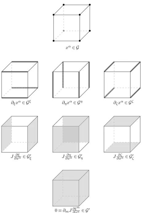
4. In 3D, we will denote the set of grid nodes by G, the grid’s edges in thel-direction byGl, the grid’s faces parallel to the lm-plane by Glm, and the grids cell-centers by Glmn. Often, we will also use a dual notation. The grid’s cell-centers can be denotedG0, the grid’s faces normal to thel-direction by Gl0, the grid’s edges normal to thelm-plane byGlm0 , and the grid’s nodes byGlmn0 . For an illustration of these centerings, see table 2.1. In 2D, this set of symbols reduces toG,Gl,Glm andG0,G0
l,G 0 lm. In 3D, the basic operators of vector calculus, written in a covariant (coordinate-independent) way, is summarized by [27, Ch. 21]
Operator domain→range formula
Gradient scalars→vectors (∇φ)m=gmn∂ nφ
Curl vectors→vectors (∇ ×~u)m=εmpq∂puq
Divergence vectors→scalars ∇ ·~u=J1∂mJ um Laplacian scalars→scalars ∇2φ= 1
J∂mJ gmn∂nφ.
by J before computing partial derivatives. The Laplacian is simply the contraction of the divergence and gradient and is not effected by these alterations.
Our discretization of geometric quantities and differential operators must befreestream preserving, mean-ing they cannot impose a bias on the direction of simple flows based on the direction of the grid lines. Also, when enforcing the incompressibility condition, we will require our velocity vector to be expressed as the sum of an irrotational component and a solenoidal component, both of which are defined using our discrete operators. These issues will be the focus of this chapter.
Section 2.1: Freestream preserving metric discretization
The choice of discretization of the Jacobian elements and metric tensor significantly impacts the long-term accuracy and stability of our numerical solutions. To illustrate this, consider the velocity advection equation,
∂uα ∂t +
1 J∂mJ u
muα= 0 (2.1)
in a 2D domain with periodic BCs. We will set the Cartesian components of the initial velocity to (U,0), whereU is uniform and constant. The single non-trivial component of the evolution equation becomes
0 =∂mJ umU=U2∂mJ ∂ξm
∂x ,
or simply
0 =∂mJ ∂ξm
∂x . (2.2)
This equation is no longer a dynamical evolution equation, but a requirement that must be satisfied by the Jacobian elements. If this equation does not hold, then a uniform velocity field will not remain so because the construction of the curvilinear grid will impose a bias on the dynamics, resulting in inaccuracies and potential instabilities that can grow in time. Note that if we were to choose an initial velocity whose Cartesian components read (0, V), then we would have arrived at a similar restriction,
0 =∂mJ ∂ξm
∂y . (2.3)
We can combine eqs. 2.2 and 2.3 into the more consise requirement,
0 =∂mJ ∂ξm
A discretization of the Jacobian elements and operators that respect eqs. 2.4 exactly is called a freestream-preserving discretization.
Equations 2.4 will be satisfied if
J ∂ξ
∂xα = ∂ηFα J ∂η
∂xα =−∂ξFα,
for some set of functions,Fα. To arrive at these functions, let us explicitly write out the Jacobian and inverse Jacobian elements, [J] = ∂x ∂ξ ∂x ∂η ∂y ∂ξ ∂y ∂η
, [J] −1=1
J ∂y ∂η − ∂x ∂η −∂y∂ξ ∂x∂ξ
, J= det([J]).
Now, we requre the inverse Jacobian elements of this coordinate mapping to be identically equal to the Jacobian elements of the inverse coordinate mapping. That is,
[J]−1= 1 J ∂y ∂η − ∂x ∂η −∂y∂ξ ∂x ∂ξ = ∂ξ ∂x ∂ξ ∂y ∂η ∂x ∂η ∂y .
This produces useful relations among the various Jacobian elements. In particular, we have the following four relations,
J∂x∂ξ = ∂η∂y J∂ξ∂y=−∂x ∂η J∂x∂η=−∂y∂ξ J∂η∂y= ∂x∂ξ
(2.5)
which provides the two functions,Fx=y andFy=−x, that were needed to satisfy eqs. 2.4. We must now investigate how to compute∂xα/∂ξm.
as follows
∂mJ ∂ξm ∂x i,j =
∂ξJ∂ξ ∂x
i,j +
∂ηJ ∂η ∂x i,j = 1 ∆ξ J∂ξ ∂x i+1/2,j − J∂ξ ∂x
i−1/2,j
! + 1 ∆η J∂η ∂x i,j+1/2 − J∂η ∂x
i,j−1/2
! = 1 ∆ξ ∂y ∂η i+1/2,j − ∂y ∂η
i−1/2,j
! − 1 ∆η ∂y ∂ξ i,j+1/2 − ∂y ∂ξ
i,j−1/2
!
= 1
∆ξ
y
i+1/2,j+1/2−yi+1/2,j−1/2 ∆η
−
y
i−1/2,j+1/2−yi−1/2,j−1/2 ∆η
− 1 ∆η
y
i+1/2,j+1/2−yi−1/2,j+1/2 ∆ξ
−
y
i+1/2,j−1/2−yi−1/2,j−1/2 ∆ξ
= 0.
Interpereted as a finite volume discretization, we have constructed the cell averages of∂mJ ∂ξm/∂x to be identically zero. A similar result holds for the cell averages of ∂mJ ∂ξm/∂y. This necessitates a specific discretization of the divergence, which will be discussed in section 2.2.
In 3D, the construction is similar, but a bit more care needs to be taken. Eqs. 2.5 must be expressed as a curl, J∂ξ ∂x= 1 2
∂η y∂ζz−z∂ζy−∂ζ(y∂ηz−z∂ηy) (2.6) J∂η
∂x= 1 2
∂ζ y∂ξz−z∂ξy−∂ξ y∂ζz−z∂ζy (2.7) J∂ζ
∂x= 1 2
∂ξ(y∂ηz−z∂ηy)−∂η y∂ξz−z∂ξy , (2.8)
so that divergences are identically zero. The remaining six formulas result from cyclic permutation ofx,y, andz. Notice that we also chose a gauge that is symmetric in all of the coordinates. Next, we must construct a discretization of these formulas.
We again evaluate xα at all nodes in G, followed by the computation of averages of partial derivatives, ∂mxα over all edges in Gm in a manner analogous to the 2D setup. Now, using the 3D identities 2.6, we generate the averages ofJ ∂ξm/∂xα over each face inG0
• • • • • • • •
xα∈ G
∂ξxα∈ Gξ ∂ηxα∈ Gη ∂ζxα∈ Gζ
J∂x∂ξα ∈ Gξ0 J
∂η
∂xα ∈ Gη0 J ∂ζ ∂xα ∈ Gζ0
0≡∂mJ∂ξ
m
∂xα ∈ G0
Table 2.1: The locations of various geometric quantities in a grid cell.
With this construction, eq. 2.4 is satisfied as follows
∂mJ ∂ξm ∂x i,j,k =
∂ξJ ∂ξ ∂x i,j,k +
∂ηJ ∂η ∂x i,j,k +
∂ζJ ∂ζ ∂x i,j,k = 1 ∆ξ J∂ξ ∂x i+1/2,j,k − J∂ξ ∂x
i−1/2,j,k
! + 1 ∆η J∂η ∂x i,j+1/2,k − J∂η ∂x
i,j−1/2,k
!
We define
A=y∂ξz−z∂ξy B=y∂ηz−z∂ηy C=y∂ζz−z∂ζy
so that
∂mJ ∂ξm ∂x i,j,k = 1 2∆ξ
∂ηC−∂ζB
i+1/2,j,k−
∂ηC−∂ζB
i−1/2,j,k
+ 1 2∆η
∂ζA−∂ξC
i,j+1/2,k−
∂ζA−∂ξC
i,j−1/2,k
+ 1 2∆ζ
∂ξB−∂ηAi,j,k+1/2−∂ξB−∂ηAi,j,k−1/2
= 1
2∆ξ
C
i+1/2,j+1/2,k−Ci+1/2,j−1/2,k
∆η −
Bi+1/2,j,k+1/2−Bi+1/2,j,k−1/2 ∆ζ
−
C
i−1/2,j+1/2,k−Ci−1/2,j−1/2,k
∆η −
Bi−1/2,j,k+1/2−Bi−1/2,j,k−1/2 ∆ζ
+ 1 2∆η
A
i,j+1/2,k+1/2−Ai,j+1/2,k−1/2
∆ζ −
Ci+1/2,j+1/2,k−Ci−1/2,j+1/2,k ∆ξ
−
A
i,j−1/2,k+1/2−Ai,j−1/2,k−1/2
∆ζ −
Ci+1/2,j−1/2,k−Ci−1/2,j−1/2,k ∆ξ
+ 1 2∆ζ
B
i+1/2,j,k+1/2−Bi−1/2,j,k+1/2
∆ξ −
Ai,j+1/2,k+1/2−Ai,j−1/2,k+1/2 ∆η
−
B
i+1/2,j,k−1/2−Bi−1/2,j,k−1/2
∆ξ −
Ai,j+1/2,k−1/2−Ai,j−1/2,k−1/2 ∆η
≡0.
Note that this is completely independent of the discretization ofA,B, andC. The cell-averaged divergences ofJ ∂ξm/∂yandJ ∂ξm/∂y can be made identically zero by similar construction.
We must now discretize J so that we can obtain the inverse Jacobian elements, ∂ξm/∂xα. We are free to choose any useful, face-averaged discretization ofJ without sacrificing freestream preservation as long as we define the inverse Jacobian determinant via 1/J. That is, the discretized versions of 1/J andJ must be exact multiplicative inverses of one another.
averages of the overlying values of J on the finer grids. However, J itself may be computed using any second order stencil that is convenient. Therefore, we simply compute the cell-centered determinant of the Jacobian matrix from the nodal coordinate data via common second order derivative stencils. Whenever the face-centered Jacobian is needed, we use an average of the neighboring cell-centered values.
OnceJis known, the inverse Jacobian matrix elements also become available. From this, we can compute the metric tensor and its inverse,
gmn=
X
α ∂xα ∂ξm
∂xα
∂ξn and g
mn=X
α ∂ξm ∂xα
∂ξn ∂xα.
The metric tensor itself turns out to not be of dynamical interest, whereas the inverse metric tensor can be found throughout eqs. 1.20, both implicitly and explicitly. As it turns out, gmn will only be needed at cell faces,Gm0 . Therefore, the off-diagonal entries require inverse Jacobian elements that must be computed using special derivative stencils.
Section 2.2: Divergence
For eq. 2.4 to be upheld, the divergence operator must be a mappping fromGm0 toG0, applying itself to face-averaged quantities to produce cell-averaged quantities. We define the discrete divergence on a single AMR level as
1
J∂mF m
i,j,k
≈hDF~i
i,j,k (2.9)
= 1
Ji,j,k
Fi+1/2,j,kξ −Fiξ−1/2,j,k
∆ξ +
Fi,j+1/2,kη −Fi,jη−1/2,k
∆η +
Fi,j,k+1/2ζ −Fi,j,kζ −1/2 ∆ζ
.
(2.10)
ξboundary of a coarse-level cell, then the correction to that cell’s divergence is
DRF~i,j,kl =± 1 Ji,j,k
P
IF ξ,l+1 I −F
ξ,l i+1/2,j,k ∆ξ
, (2.11)
where I represents the indices of the faces that hold the fine-level fluxes andl or l+ 1 denotes the data’s AMR level. Corrections on the lower cell boundaries use the minus sign, while corrections on the upper cell boundaries use the plus sign. SinceF~ is a flux, it is assumed to be scaled byJ due to our redefinition of the divergence operator. These corrections are accumulated over the domain then applied by
DF~l←DF~l+DRFl. (2.12)
The correction term,DRF~lis called thereflux divergenceand the act of correcting the coarse-level divergence with fine-level fluxes via eq. 2.12 is calledexplicit refluxing.
If we are refluxing a diffused quantity, the we must diffuse the correction before applying it toDF~l. We perform the implicit refluxing using a backwards Euler timestep. For example, suppose F~l is a buoyancy flux andκis its (thermal) diffusivity. Then we solve
(1−∆tlκ∇2)δ ~Fl= ∆tlD RF~l,
using homogeneous BCs at the domain boundaries. If the coarse level, l, has a CF interface with another coarser level, l−1, then we assume thatδ ~Fl−1= 0 and use quadratic interpolation to fill the CF interface ghosts ofδ ~Fl. The diffused update is then applied by
DF~l←DF~l+δFl. (2.13)
Implicit refluxing not only promotes accuracy at the CF interfaces, but also ensures the stability of hyperbolic conservation laws.