Multiple Testing in Genome-Wide Studies
by Moonsu Kang
A dissertation submitted to the faculty of the University of North Carolina at Chapel Hill in partial fulfillment of the requirements for the degree of Doctor of Philosophy in the Department of Biostatistics, School of Public Health.
Chapel Hill 2007
Approved by:
Dr.Pranab K.Sen, Advisor
Dr.Chirayath Suchindran, Reader Dr.Fei Zou, Reader
c
2007 Moonsu Kang
ABSTRACT
MOONSU KANG: Multiple Testing in Genome-Wide Studies. (Under the direction of Dr.Pranab K.Sen.)
DNA microarray technologies allow us to monitor expression levels of thousands of genes simultaneously. A basic task in analyzing microarray data is the identifica-tion of differentially expressed genes under different experimental condiidentifica-tions. The null hypothsis is no association between the expression levels and explanatory variables or covariates. Family-wise error rate (FWER), although very conservative, controls type I error. False Discovery Rate (FDR) is a less stringent approach which aims to control the expected proportion of Type I errors among the rejected hypotheses. Since there are thousands of genes tested simultaneously, FDR may be enhanced. High correlation between tested genes, attributed to co-regulations and dependency in the measurement errors, further complicates the problem. Most of the current FDR procedures assume independence or rather restrictive dependence structures, resulting in being less reli-able.
In this work, we address these very large multiplicity problems by adopting a two-stage FDR controlling procedure under suitable dependence structures and based on Poisson distributional approximation, which eliminates the need to assume restricted depen-dence structures. We compare the performance of the proposed FDR procedure with that of other FDR controlling procedures, with illustration of the leukemia microarray study of Golub et al. (1999) and simulated data. In these studies, the proposed FDR procedure has greater power without much elevation of FDR.
low sample size constraints. Using the 2002-03 SARS epidemic model, it is shown that proposed FDR procedure along with an appropriate test statistic based on a pseudo-marginal approach with Hamming distance performs better.
ACKNOWLEDGMENTS
CONTENTS
LIST OF FIGURES ix
LIST OF TABLES x
List of Abbreviations xi
1 INTRODUCTION AND LITERATURE REVIEW 1
1.1 Introduction . . . 1
1.2 Literature Review . . . 3
1.2.1 Multiple Testing And Adjustedp-values . . . 3
1.2.2 Simes Inequality And M T P2 Property . . . 7
1.2.3 Control Of FWER . . . 8
1.2.4 Control Of FDR . . . 11
1.2.5 Recent Proposals For DNA Microarray Experiments . . . 21
1.2.6 Classification Of Genes . . . 23
1.2.7 The Chen-Stein Method . . . 24
1.3 Overview of Research . . . 25
2 FALSE DISCOVERY RATE IN MICROARRAY STUDIES 28 2.1 Dependence structures among tested genes . . . 28
2.1.1 Introduction . . . 28
2.1.2 Model . . . 30
2.1.4 Stochastic ordering . . . 32
2.1.5 Monotonicity property of FDR . . . 35
2.1.6 FNR . . . 36
2.1.7 Monotonicity property of FNR . . . 36
2.2 Two stage FDR procedure . . . 37
2.2.1 Introduction . . . 38
2.2.2 Model . . . 38
2.2.3 Distributions . . . 39
2.2.4 F DR(2) . . . 40
2.2.5 Stochastic ordering . . . 44
2.2.6 Monotonicity ofF DR(2) . . . 48
2.2.7 F N R(2) . . . . 50
2.2.8 Monotonicity ofF N R(2) . . . . 50
2.2.9 Control of FDR . . . 51
2.2.10 Estimation procedure . . . 52
3 FALSE DISCOVERY RATE IN GENOMIC SEQUENCES 54 3.1 Introduction . . . 54
3.2 A Pseudo Marginal Model . . . 56
3.2.1 Proposed Test Statistics and P-values . . . 57
3.3 Discussion . . . 58
3.3.1 False discovery rate optimality and Average Power . . . 60
4 CLASSIFICATION OF GENES 63 4.1 Introduction . . . 63
4.2 Proposed Test Statistics and P-values . . . 64
4.2.2 Linear Rank Statistics . . . 64
4.2.3 A Marginal Model Based On Kendall tau statistics . . . 72
4.2.4 Robust M-test . . . 73
5 NUMERICAL STUDY 83 5.1 Numerical Study of FDR in DNA microarray experiment . . . 83
5.1.1 Independence example . . . 84
5.1.2 Dependence example . . . 86
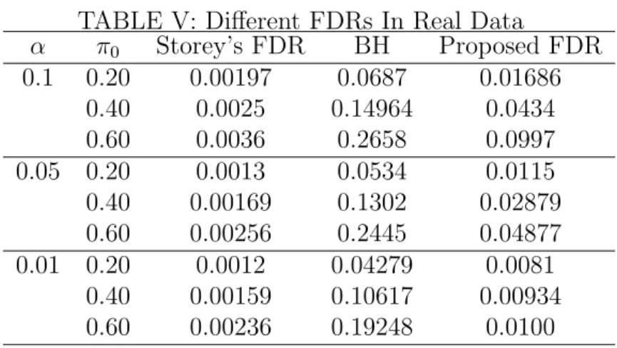
5.1.3 Application to Real Data: Leukemia study . . . 90
5.2 FDR in genomic sequences . . . 96
5.2.1 Application to The SARSCoV RNA Genome . . . 96
5.3 Numerical Study in Classification Of Genes . . . 98
5.3.1 Application To the Breast Cancer Study . . . 99
6 SUMMARY AND FUTURE RESEARCH 104 6.1 Summary and Conclusion . . . 104
6.2 Discussion and Future Research . . . 106
Appendix
108
LIST OF FIGURES
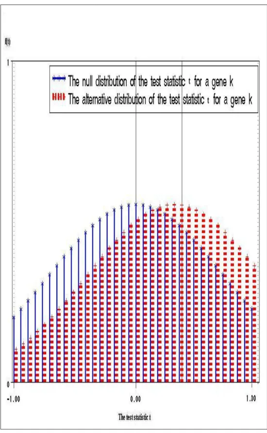
I Comparison of the null distribution with the alternative distribution . 62 I Comparison of Average Power for different FDR procedures
(Indepen-dence) . . . 88
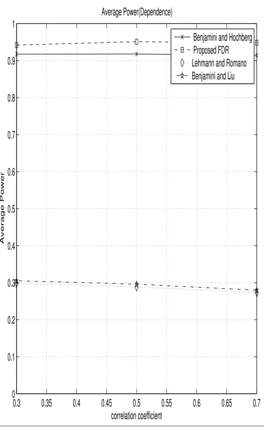
II Comparison of Average Power for different FDR procedures (Depen-dence) . . . 89
III Comparison of arrays . . . 93
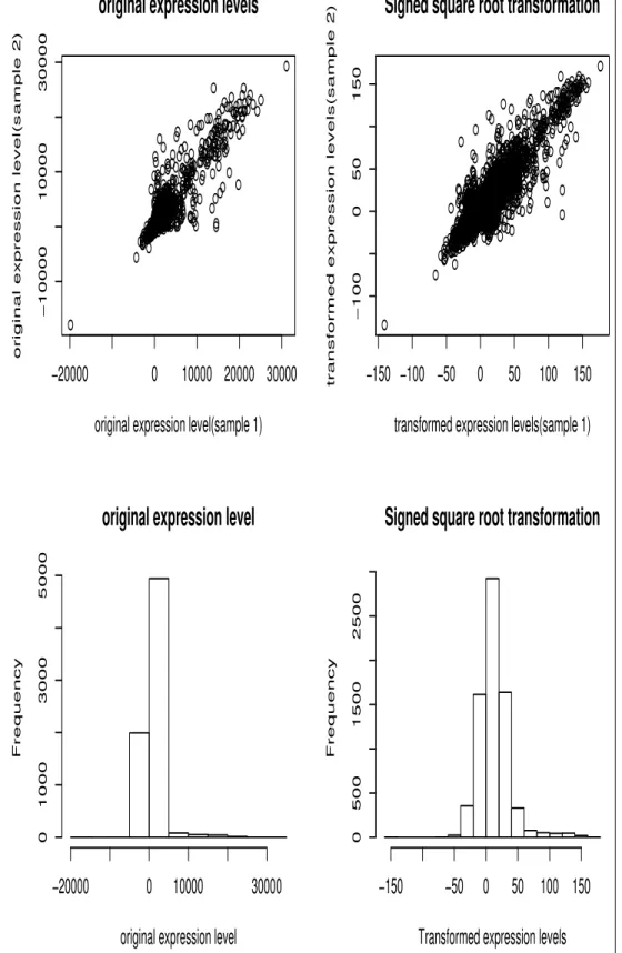
IV Comparions of expression level with signed square root transformation of expression level . . . 94
V Distribution of p-value (Real data) . . . 95
VI The SARSCoV RNA Genome . . . 96
VII Mean expression levels for monotone profiles . . . 100
LIST OF TABLES
I Number of errors committed when testing m null hypotheses . . . 5
I Comparison of different FDR procedures (Independence) . . . 85
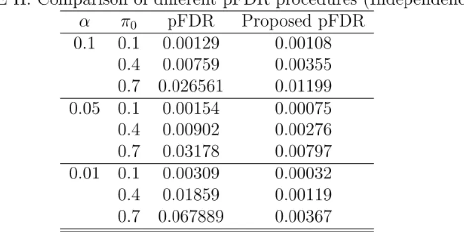
II Comparison of different pFDR procedures (Independence) . . . 85
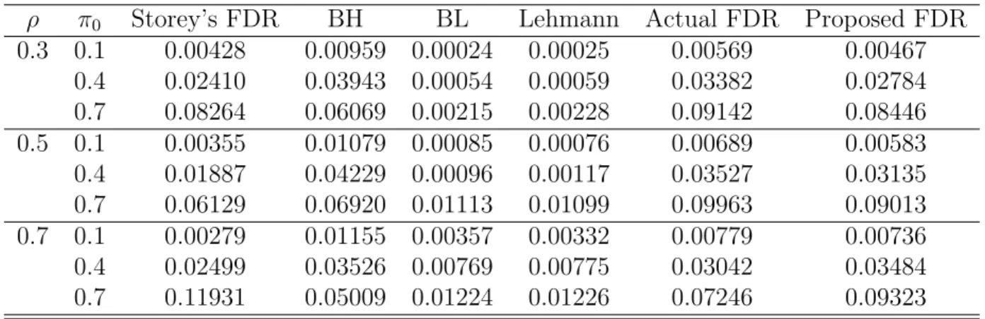
III Comparison of different FDR procedures (Dependence) . . . 87
IV Comparison of different pFDR procedures (Dependence) . . . 87
V Different FDRs In Real Data . . . 91
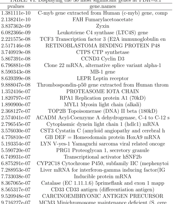
VI Displaying the 30 most significant genes at FDR=0.1 . . . 92
VII Modified FDR at π0 = 0.4 . . . 92
VIII Comparison of different pFDR procedures (Real data):Golub et al. . . . 96
IX Comparison of different FDR procedures-Hamming distance . . . 98
X Comparison of different pFDR procedures-Hamming distance . . . 98
XI Comparison of different FDR procedures (Breast data): . . . 102
List Of Abbreviations
• MTP2 : X has M T P2 property if for all x and y, f(x)·f(y) ≤ f(min(x,y))· f(max(x,y)), where f is the joint density and the minimum and maximum are evaluated componentwise.
• TP2 : A nonnegative bivariate function f ( x , y) is said to be T P2 in ( x , y)
if the following condition holds: f ( x , y ) f (x’, y’) 2 f ( x , y’)f (x’, Y ) for all
x < x0 and y < y0.
• PRDS : A multivariate distribution is said to have positive regression depen-dency (PRDS) if for any increasing set D, P(X ∈ D|X1 = x1, . . . , Xi = xi) is
CHAPTER 1
INTRODUCTION AND
LITERATURE REVIEW
1.1
Introduction
The Human Genome Project announced the completion of a map of the human genome in 2003. DNA microarrays are used to measure the level of expression of genes under different enviromental setups by hybridizing a labeled cRNA representation of the mRNA to cDNA sequences (cDNA microarrays) or by hybridizing a labeled cRNA representation of the mRNA to short specific segments (synthetic oligonucleotide mi-croarrays).
procedure along with an appropriate test statistics to microarray experiment as well as categorical genomic sequences in Chapters 2 and 3.
The high-dimension (K) low sample size (n) environments make it hard to classfiy thou-sands of genes. These problems make it unreasonable to adopt standard models where the number of parameters outnumber the sample size. Studies such as dose-response microarray experiments or time-course data mainly involves order-restricted inference. In these enviroments, Roy’s (1953) union-intersection principle have some advantanges (Silvapulle and Sen 2004, Tsai and Sen 2005). Based on the Union-Intersection prin-ciple, robust M-statistics , insensitive to outlier arrays, and linear rank statistics, a locally most powerful test, is proposed in Chapter 4. The real microarray datasets, real genomic sequence and simulation models are presented in Chapter 5 to evaluate proposed FDR and the corresponding test statistics. Overview of research work on this problems is summarized in section 1.3.
1.2
Literature Review
1.2.1
Multiple Testing And Adjusted
p
-values
1.2.1.1 Multiple Testing In DNA Microarray Experiments
Define multiple hypotheis testing procedure in microarray experiment. An m × n
matrix X = (xji) = (X1, . . . , Xm) represents the gene expression level data with rows
corresponding to genes and columns corresponding to individual microarry experiments. The expression measuresxji are in general highly preprocessed data. We use the sample
data {(xi, yi)}i=1,...,n formed by the expression profiles xi and response or covariates yi
in order to test hypotheses regarding the joint distrubution of the expression measures
X = (X1, . . . , Xm) and response or covariate Y. A standard approach to the multiple
testing problem includes two aspects:
• computing an appropriate test statsisticTj for each gene j,
• applying a multiple testing procedure to determine which hypotheses are rejected while controlling a suitably defined Type I error rate.
1.2.1.2 Type I Error Rates
A multiple testing procedure controls a particular Type I error rate at level α if this error rate is less than or equal to α when the given procedure is applied to a set of rejected hypotheses.
Consider the problem of simultaneous testingmnull hypotheses,Hj, j = 1, . . . , mwhich
are assumed to be known, of which m0 are true and unknown. The corresponding p
-values are P1, . . . , Pm. This situation can be expressed by the table below. R is the
number of hypotheses rejected, which is an observable random variable. U, V, S, andT
are unobservable random variable.
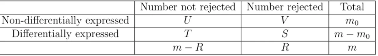
TABLE I: Number of errors committed when testing m null hypotheses Number not rejected Number rejected Total
Non-differentially expressed U V m0
Differentially expressed T S m−m0
m−R R m
In the microarray setting, there is a null hypothesisHifor each geneiand rejection ofHi
corresponds to declaring that gene i is differentially expressed. In general, we’d like to minimize the numberV corresponding to Type I error and the numberT corresponding to Type II error. When testing a single hypothesis H, the probability of Type I error is controlled at prespecified level α. This may be achieved by choosing a critical value
cα so that P r(|T| ≥cα|H) ≤ α and rejecting the null hypothesis when |T|> cα. The
Type I error rates shown below are the most standard ones Shaffer (1995).
• The per-comparison error rate (PCER):the expected value of the number of Type I errors divided by the number of hypotheses, that is,P CER=E(V)/m.
• The per-family error rate (PFER):the expected number of Type I errors, E(V).
• The family-wise error rate (FWER):the probability of at least one Type I error, that is,F W ER =P r(V ≥1).
• The false discovery rate (FDR) of Benjamini and Hochberg (1995):the expected proportion of Type I errors among the rejected hypotheses.
It is easy to prove that P CER ≤ F DR ≤ F W ER ≤ P F ER. Note that the error rates are defined under the true and typically unknown data generating distribution for gene expression data X = (xji) = (X1, . . . , Xm) where a gene expression profile is
of null hypotheses is true for this distribution. Weak control refers to control of Type I error rate when all the null hypotheses are true. In the microarray setting, it seems more appropriate to have strong control of the Type I error rate, that is, control under any combination of true and false null hypothesis.
1.2.1.3 Adjusted p-values
The multiple testing procedure may be defined in terms of unadjusted p-values or adjusted p-values. Unadjusted p-value gives the probability of obtaining a value of a test statistic that is at least as unfavorable to H0 as the observed one, that is, pj = P r(|Tj| ≥ |tj||Hj) for hypothesis Hj. The adjusted p-value for Hj is defined as
the nominal level of the entire test procedure at which Hj to be rejected, provided
that the values of all test statistics are given. For FWER controlling procedure, ˜pj is
defined as inf{α∈[0,1] :Hj is rejected at nominalF W ER=α}. For FDR controlling
procedure, ˜pj is defined as inf{α∈[0,1] :Hjis rejected at nominalF DR =α}(Yekutieli
1.2.2
Simes Inequality And
M T P
2Property
To test the overall null hypothesis H0 =Tni=1Hi with their correspondingP values
at a prespecified significance level α is a common problem in practice. For example, when identifying differentially expressed genes, multiple studies are often performed: the simultaneous multiple test for each gene. Type I error should be controlled at preassigned level in multiple testing procedure. Simes method is one of the methods to control type I error. We intend to identify the correlation structure among the genes. It is said thatM T P2 property may characterize a general class of positive dependence
structures among the genes. We introduce this concept along with positive regression dependence.
The classical and well-known Bonferroni method rejects H0 IF Pi ≤ α/m for at least
one i. But this method is very conservative, particulary when the dependence among the test statistics is very high. Simes (1986) proposed modified Bonferroni methods. LetP(1) ≤, . . . ,≤P(m) be the ordered P values. Simes suggested the test procedure to
reject H0 if Pi ≥ iαm at least one i. Under Simes inequality, this method controls the
typeI error rate for the test statistics having the folllowing distributions.
The null distributions of test statistics, X1, . . . , Xm, have probability densities of the
form
Z m Y
i=1
f(xi, z)g(z)dz (1)
for some probability densitiesf(x, z) andg(z), wheref(x, z) isT P2 in (x, z). Statistics
distribu-tions have densities of the form (1). The following M T P2 property Karlin and Rinott
(1980) characterizes a class of positive dependent distribution. A multivariate distri-bution is said to have positive regression dependency (PRDS) if for any increasing set
D, P(X ∈ D|X1 = x1, . . . , Xi = xi) is nondecreasing in (x1,· · · , xi). A stricter
con-dition, that is, positive regression dependency, is multivariate total positivity of order 2, M T P2 if for all x and y, f(x)·f(y) ≤f(min(x,y))· f(max(x,y)) where f is either the joint density or the joint probability function, and the minimum and maximum are evaluated componentwise.
LetX(1), . . . , X(m)be the ordered values of a set ofM T P2 random variablesX1, . . . , Xm
with a marginal F. Then P r(X(j) ≤ aj, j = 1, . . . , m) ≤ 1−α. If {aj} are such that
F(aj) = jαm, with the equality holding when when {Xi} are independent. The Simes
inequality holds in general for all M T P2 distributions. However, Karlin and Rinott
(1980) considered the strongly multivariate reverse rule of order two (S−M RR2)
con-dition characterizing negatively dependent multvariate distributions. They proved that the Simes conjecture is not true in general for such distributions.
1.2.3
Control Of FWER
The common approach to the multiplicity problem is to control the FWER at preas-signed level. The FWER is said to be controlled at level α by a particular multiple testing procedure if FWER≤α. We shall introduce the existing FWER methodologies here.
• Single-step procedures: Strong control of FWER is provided based on Boole’s inequality.
F W ER=P r(V ≥1) =P r(
m0
[
j=1
{P˜j ≤α})≤ m0
X
j=1
P r( ˜Pj ≤α) = m0
X
j=1
P r(Pj ≤
α
m)≤
m0α
m .
fol-lowing ˜Sid´ak’s procedure controls for FWER for test statistics that satisfy the ˜
Sid´ak’s inequality.
P r(|T1| ≤c1, . . . ,|Tm| ≤cm)≤ m
Y
j=1
P r(|Tj| ≤cj).
The single-step ˜Sid´ak’ adjusted p-values are given by ˜pj = 1−(1−pj)m.
Westfall and Young (1993) proposed adjusted p-values for less conservative pro-cedures which take into account the dependence structure among test statistics. The single-step min P adjustedp-values are given by
˜
pj =P r(min1≤l≤mPl ≤pj|H0C).
The single-step maxT adjusted p-values are given by
˜
pj =P r(max1≤l≤mTl ≤tj|H0C).
• Step-down procedures: Step-down FWER procedures achieve higher power rather than by single-step procedures. Let pr1 ≤ pr2 ≤ · · · ≤ prm denote the observed
ordered unadjustedp-values andHr1, Hr2, . . . , Hrm denote the corresponding null
hypotheses. The Holm (1979) procedure operates in the following manner. Define
j∗ =min{j :prj > α/(m−j+1)}and reject hypothesesHrj, forj = 1, . . . , j ∗−1.
If no suchj∗ exists, reject all hypotheses. Similarly, the step-down Holm adjusted
p-values are given by ˜prj = maxk=1,...,j{min((m−k+ 1)prk,1)}. The step-down
˜
Sid´ak adjusted p-values are defined as ˜prj = maxk=1,...,j{1−(1−prk)
(m−k+1)}.
The Westfall and Young (1993) step-down min P adjusted p-values are defined by
˜
prj =maxk=1,...,j{P r(minl∈{rk,...,rm}Pl ≤prk|H
C
And the step-down maxT adjusted p-values are defined by
Pp˜rj =maxk=1,...,j{P r(maxl∈{rk,...,rm}|Tl| ≥ |trk||H
C
0 )}.
where|tr1| ≥ |tr2| ≥ · · · ≥ |trm| denote the observed ordered test statistics.
• Step-up procedures: Under the complete null hypothesisHC
0 and for independent
test statistics, the ordered unadjusted p-values P(1) ≤ P(2) ≤ · · · ≤ P(m) satisfy P r(P(j) ≥ jαm, ∀j = 1, . . . , m|H0C) ≥ 1−α with equality in the continuous
case. Step-up procedures start with this Simes inequality (1986). Hochberg (1988) applied the Simes inequality to derive the following FWER controlling procedure. Letj∗ =max{j :prj ≤α/(m−j+ 1)}and reject hypothesesHrj, for j = 1, . . . , j∗. If no such j∗ exists, reject no hypotheses. The step-up Hochberg adjustedp-values are given by ˜prj =mink=j,...,m{min(m−k+ 1)prk,1)}.Related
procedure are those of Hommel (1988) and Rom (1990). All procedures based upon the Simes inequality have the assumption that the result derived under independence is a conservative procedure for dependent tests.
However, Benjamini and Hochberg (1995) argued that this FWER approach has the following limitations.
• Much of the methodology of FWER controlling procedures is concerned with com-parisons of multiple treatments and families whose test statstics have multivariate normal (ort).
• Strong control of the FWER tends to be less powerful than the per comparison procedure of the same levels.
In many situations, control of the FWER is too restrictive at the expense of substan-tially lower power in detecting false hypotheses. One may wish tolerate some Type I errors, provided their number is small in comparison to the number of rejected hy-potheses.
1.2.4
Control Of FDR
As we have seen before, control of the FWER is too conservative when there are many hypotheses such as in microarray experiments. The number of erroneous re-jections should be considered in many multiplicity problems. At the same time, the seriousness of the loss by erroneous rejections is related to the number of rejected hy-potheses.
Benjamini and Hochberg (1995) introduced the concept of the false discovery rate (FDR) in order to control for the conservativeness of the FWER. Let the unobserved random variableQ= VV+S-the proportion of the rejected null hypothses which are erro-neously rejected. Q= 0 when V +S=0. We define the FDR Qe to be the expectation
of Q, Qe =E(Q) =E{VV+S}=E{VR}. Under the complete null hypotheses, control of
the FDR implies control of the FWER in the weak sense. Whenm0 < m, the FDR is
smaller than or equal to the FWER.
Benjamini and Hochberg (1995) proposed the following step-up FDR controlling proce-dure. Consider testing H1, H2, . . . , Hm with the corresponding p-values P1, P2, . . . , Pm.
LetP(1) ≤P(2) ≤, . . . ,≤ P(m) be the ordered p-values, and denote by H(i) the null
hy-pothesis corresponding to P(i). Define the following Bonferrroni type multiple-testing
procedure :
Benjamini and Liu (1999) derived a new step-down procedure when test statistics are independent. Define the m critical values by
δi ≡1−[1−min(1,
m
(m−i+ 1)q)]
1
(m−i+1) ,1≤i≤m.
The step-down procedure then operates as follow . Let k be the smallest i for which
P(i) > δi. RejectH(1), . . . , H(k−1). This procedure controls the FDR at levelqBenjamini
and Liu (1999). They proved that their procedure neither dominates nor is dominated by the step-up procedure.
Benjamini and Yekutieli (2001) showed that if the joint distribution of the test statis-tics is PRDS on the subset of test statisstatis-tics corresponding to true null hypotheses, the Benjamini-Hochberg procedure controls the FDR at less than or equal to m0mq. They also introduced a simple conservative modification of the procedure which controls the FDR for arbitrary dependence structures. Adjustedp-values for this modified step-up procedures are ˜prj =mink=j,...,m{min(
mPm j=11/j
k prk,1)}.
Choosing the critical valuesc1 ≤ · · · ≤cm subject to a preassigned levelα, is equivalent
to finding constants a1 ≤ · · · ≤ am satisfying the following set of inequalities Sarkar
(2000):P(X1:k ≤ a1, . . . , Xk:k ≤ ak)≥ 1−α where X1:k ≤ . . . Xk:k denote the ordered
components of (X1, . . . , Xk). Finner and Roters (1998) illustrated this, which provided
that the critical values (a1 ≤ a2 ≤ a3) satisfying this inequality involving an equicor-related trivariate standard normal distribution is in fact monotone when the common correlation is positive and at most (z2
α/2−z 2 1/4)/(z
2
α/2+z 2
1/4), where zα/2 is the upper
100α percent point ofN(0,1). This example is generalized to the fact that the desired monotonicity property holds in general for M T P2 test statistics.
explicit expression of the FDR of a generalized step-up-step-down procedure of orderr, in terms of right-tailed test based onX1, . . . , Xm with the corresponding critical values
c1, . . . , cm. Starting with the formulaF DR=Pi∈I0
Pm−1
j=0 1
m−jP[{Xi ≥c(j+1)}]∩B r j,m,
where{Hi, i∈I0}is the list of true null hypotheses.
F DR = 1
m−r+ 1
X
i∈I0
P{Xi ≥c(r)}
+ X
i∈I0 r−1
X
j=1
E[φrj,m(Xi)(
I(Xi ≥c(j))
m−j+ 1 −
I(Xi ≥c(j+1))
m−j )]
+ X
i∈I0 m−1
X
j=r
E[Ψrj,m(Xi)(
I(Xi ≥c(j+1))
m−j −
I(Xi ≥c(j))
m−j+ 1 )
with φr
j,m(Xi) = P{X(j)≥c(j), . . . , X(r) ≥c(r)|Xi}
and Ψr
j,m(Xi) =P(X(r) < c(r),· · · , X(j)< c(j)|Xi).Sarkar (2004)
Under a variety of distributional settings of the Xi0s, the c0(i)s can be obtained such that the FDR in above formula is controlled at less than or equal to m0α/m, and
hence less than or equal to α. For example, when the Xi0s are stochastically inde-pendent, or have a multivariate distribution exhibiting a positive dependence propo-erty in the sense that the Xi0s are PRDS on the subset {Xi, i ∈ I0}, c
0
(i)s satisfying F(c(i)) = 1− (m− i+ 1)α/m, i = 1, . . . , m with F(·) being the common marginal
null cumulative distribution function of the Xi0s, provide a control of the FDR at
α (Sarkar,2002). These are the Simes (1986) critical values used in the Benjamini-Hochberg step-up test with independent test statistics. It is important to note that the step-up test with these critical values in the independent case is actaully exactly equal tom0α/m (Benjamini and Yekutieli 2001; Finner and Roters 2001; Sarkar 2002).
step-down procedure are such that F(c(i)) =
1−min(1,mi α)1/i, i = 1, . . . , m. This step-down procedure controls the FDR atα for the independent statistics. Sarkar (2002) has strengthened this fact by proving that the FDR-controlling property still holds when the test statistics are positively dependent in the sense of being M T P2
under any alternatives, and exchangeable under the null distribution.
The proportion of false negatives among the accepted null hypotheses is defined as
N =T /A ifA >0 and = 0 ifA= 0, and then we define the false negatives rate (FNR) by E(N). The FNR of a generalized step-up-step-down procedure of order r is given by
F N R = 1
r
X
i∈I1
P{Xi ≤c(r)}
+ X
i∈I1 r
X
j=2
E[φrj,m(Xi){
I(Xi ≤c(j))
j−1 −
I(Xi ≤c(j))
j }]
+ X
i∈I1 n
X
j=r+1
E[Ψrj,m(Xi){
I(Xi ≤c(j))
j −
I(Xi ≥c(j−1))
j−1 }]
Sarkar (2004) A step-down procedure can be used to control the FNR under certain conditions, for example, independence or PRDS, on the test statistics.
The difference 1−(F DR+F N R) indicates the strength of unbiasedness as well as a measure of power of a multiple testing procedure. Between two procedures, the one with higher value of this difference is more powerful, in that it maintains either a higher proportion of corretly accepted null hypotheses or a low proportion of falsely rejected null hypotheses. Based on simulation data from equi-correlated multivariate normals, the performance of the Benjamini-Hochberg test performs better than any other step-up-step-down test.
repre-senting how the results show FDR-or-FNR-controlling single-step procedure, like Bon-ferroni or Sidak procedure, can be improved by borrowing information about m0 or
m1 in the sprit of Benjamini and Hochberg (2000), Benjamini, Krieger, and Yekutieli (2002), Storey (2002) and Storey, Taylor, and Siegmund (2004). Storey, Taylor, and Siegmund (2004) provided procedures modifying the BH procedure using estimates of
m0 and proved that they control the FDR under independence. Two families of proce-dures ,one modifying the FDR-controlling and the other modifying the FNR-controlling Sidak procedures are proposed. These control FDR or FNR under independence less conservatively than the corresponding families modifying the FDR-or FNR-controlling Bonferroni procedure by using the estimates of m0 considered in Storey, Taylor, and
Siegmund(2004). Sarkar extends Storey’s (2002, 2003) result to dependent case by considering a mixture model where different configurations of true and false null hy-potheses are assumed to have certain probabilities Sarkar (2004).
However, it was shown that most of all FDR controlling procedures were shown to control the FDR in cases of restricted dependency but they were not designed to make use of the dependency structure to gain more power when possible. Denote the true null hypotheses by {H01, . . . , H0m0} and the false null hypotheses by {H11, . . . , H1m1}.
The corresponding vectors of p-values are P0 and P1, respectively. Knowing how P0 is distrubuted, we can construct more powerful MCPs. Resampling-based FDR con-trolling procedure along the line of Westfall and Young(1993) for FWE control, use
The BH FDR local estimator is defined asQBH est (p) =
m·p/r(p) if r(p)≥1
0 otherwise
Based on the resampling-based distributionR∗, Benjamini and Yekutieli also introduced two resampling-based estimators differing in their treatment of s(p): point estimator and an upper limit. The first estimator is r(p) −mp. Using this downward biased estimator, the resampling-based FDR local estimator is given by
Q∗(p) =
ER∗ R
∗(p)
R∗(p)+r(p)−p·m if r(p)−rβ∗(p)≥p·m
P rR∗{R∗(p)≥1} otherwise
The second estimator is r(p)-rβ∗(p), assuming subset pivotality conditioning on
S(p) = s(p), The resampling based 1−β FDR upper limit is defined as
Q∗β(p) =supx∈[0,p]
ER∗ R
∗(p)
R∗(p)+r(p)−r∗
β(p) if r(p)−r ∗
β(p)≥0
P rR∗R∗(p)≥1 otherwise
Based on ˆQ, the FDR local estimator computed, the size q MCP based on the FDR local estimator is :if kq = maxk{Qˆ(p(k) ≤q}, reject H(1)0 , . . . , H(0kq) Yekutieli and
Ben-jamini (1999).
The traditional FDR controlling procedures involve sequentialp-value rejection meth-ods. For example, Benjamini and Hochberg (1995) provided a sequential p-value method. A sequential p-value method gives us an estimate ˆk that leads to reject
p(1), p(2), . . . , p(ˆk), where p(1) ≤ p(2) ≤ · · · ≤ p(ˆk) are the ordered observed p-values.
However, ˆk may not be reliable case by case. Secondly, the method controls the error rate for all possible values ofm0, which is the number of true null hypotheses simulta-neously without any information about m0. Instead of fixing the error rate and then estimating k, we propose the opposite approach to fix the rejection region and then estimate α.
the conditional FDR given that there is at least one rejection. pFDR protects false discovery better than FDR since it is conditioned on the occurence of discovery. Let
F DR(t) denote the FDR when rejecting all null hypotheses withpi ≤tfori= 1, . . . , m.
Fort∈[0,1], letV(t), S(t), andR(t) denote the number of{null pi :pi ≤t}, the
num-ber of{alternativepi :pi ≤t}, andV(t)+S(t), respectively. In terms of these empirical
processes, F DR(t) = E[RV(t()t∨)1]. Similarly, pF DR=E(RV((tt))|R(t)>0).
Storey proposed a bootstrap-based algorithm to control F DR and pF DR. Similarly,
pF DR(λ) is estimated by pF DRˆ (λ)(t) = ˆπ0ˆ (λ)t
P r(P≤t){1−(1−t)
m}. ForB bootstrap
sam-ples of p1, . . . , pm, caculate the bootstrap esimates pF DRˆ
∗b
λ (b = 1, . . . , B).
Form a 1−α upper confidence interval forpF DR(t) by taking the 1−αquantile of the ˆ
pF DR∗λb(t) as the upper confidence bound. Since FDR is not conditioned on at least one rejection occuring, we can setF DRˆ λ(t) =
π0(λ)t
ˆ
P r(P≤t). Tibshirani et al (2001) develop
the software package SAM applying this approach. Let’s look at the finite sample setting of m.
Theorem 1.2.1 If the p-values for the true null hypotheses are independent and have
uniform distribution, E{pF DRˆ λ(t)} ≥pF DR(t) and E{F DRˆ λ(t)} ≥F DR(t) for all
t and π0.
ˆ
F DRλ(t) and pF DRˆ λ(t) is a conservative point esimate of F DRλ(t) and pF DRλ(t),
respectively.
Storey (2002)
Theorem 1.2.2 If the p-values corresponding to the true null hypotheses are
independent, then, for λ >0, F DR{(tα(F DRˆ
∗
λ} ≤(1−λπ0m)α≤α.
Storey et al. (2004)
Hence, the thresholding procedure using F DRˆ λ(t), which is a family of conservatively
sense. So, the goals of the BH procedure and this procedure can be met with this one family of estimates.
Now, let’s look at the case when m is large. For large m, the assumption of independence can be weakened to ”weak dependence”. The following three assumptions are needed for large m results.
limm→∞{Vm0(t)} =G0(t), limm→∞{ S(t)
m1
}=G1(t) a.s.t∈(0,1] (1),
0< G0(t)≤t , t∈(0,1]; (2),
limm→∞m0m ≡π0 (3).
whereG0 and G1 are continous functions.
ˆ
F DR∞λ (t) ={1−G0(t)
1−λ π0+
1−G1(t)
1−λ π1}G0(t)/{π0G0(t) +π1G1(t)}.
This is the pointwise limit ofF DRˆ λ(t) under the assumptions (1)-(3)Storey et al.
(2004).
Theorem 1.2.3 Suppose that the convergence assumptions of equations (1)−(3)
hold. For each δ >0,
limm→∞inft≥δ{F DRˆ λ−F DRλ(t))} ≥0 and limm→∞inft≥δ{F DRˆ λ− RV(t()t∨)1} ≥0
with probability 1.
Storey et al. (2004)
Hence, an estimate of F DR(t) proposed in Storey (2002) a conservative estimate of the error rate over all significance regions simultaneously in the asymptotic setting. Thus, the goals of the traditional sequentialp-value method and a new method are equivalent.
that the test statistics have a random mixture of the null and alternative
distributions, the pFDR can be restated as a simple Bayesian posterior probability as shown below. Second, these properties remain asymtotically under general conditions, even under certain form of dependence in that the realizd V /R, the FDR, and the pFDR all converge to the Bayesian form of the pFDR simultaneously over all significance regions. Third, the pFDR can be used to define the q-value, a natural pFDR analogue to the p-value.
For an observed statisticT =t, the q-value of t is defined as
q(t) = inf{Γα:t∈Γα}{pF DR(Γα)}. In words, the q-value is a measure of the strenth of
an observed statistic with respect to pFDR. The q-value is ”posterior Baysian
p-value”-the minimum posterior probability H = 0 over all significance containing the statistic. Fourth, the pFDR has a connection to classification theory, and the set of Bayes rule can be used to minimize (1−w)·pF DR+w·pF N R, where the pFNR is the natural counterpart to the pFDR,wherepF N R=E[WT |W >0].
We have shown that in both finite sample and asymptotic settings, the goals of two approaches are equivalent. Using this new approach, we reject a greater number of hypotheses while controlling the same error rate as the Benjamini and Hochberg (1995) method, which leads to higher power. If the number of tests is large, it’s appropriate to tolerate more than one false rejection provided the number of such cases is controlled, therefore increasing the ability of the procedure to detect false null hypotheses. E.L.Lehmann and J.P.Romano (2005) derived single-step and stepdown
k-FWER procedures, controlling the probability of k or more false rejections, without any assumptions about the dependence structure of the p-values Lehmann and
Romano (2005).
Theorem 1.2.4 For testing Hi :P ∈wi, i= 1, . . . , m,suppose pˆi satisfies the
that rejects any Hi for which pˆi ≤kα/s. This procedure controls the k-FWER, so that
P{pˆi ≤u} ≥P{X ∈Si(u)}. holds. Equivalently, if each of the hypotheses is tested at
level kα/s, then the k-FWER is controlled.
Theorem 1.2.5 (i) Let the αi be given below.
αi =
kα
m i≤k kα
m+k−i i > k
For any i≥k there exists a joint distribution for pˆ1, . . . ,pˆs such that m+k−i of the
ˆ
pi are uniformly distributed on (0,1) and the following holds.
P{p(1)ˆ ≤α1,p(2)ˆ ≤α2, . . . ,p(ˆi−1) ≤αi−1,p(ˆi) ≤αi}=α.
(ii) For testing Hi :P ∈wi, i= 1, . . . , m, suppose pˆi satisfies the following:
P{pˆi ≤u} ≤u for any u∈(0,1). Let α1 ≤α2 ≤ · · · ≤αm be constants. If pˆ(1) > α1,
reject no null hypotheses. If hatp(1) ≤α1, . . . ,pˆ(r) > αr, reject hypotheses
H(1), . . . , H(r). For this stepdown procedure with αi , one cannot increase even one of
the constants αi (for i≥k) without violating the k-FWER.
Lehmann and Romano (2005)
Lehmann and Romano (2005) proposed one stepdown procedure to control the FDP under mild conditions on the dependence structure of p-values. ˆp1, . . . ,pˆs denotes the
p-values of the individual tests. Also let ˆq1, . . . ,qˆ|I| denote the p-values corresponding
to the|I|=|I(P)|ture null hypotheses. Soqi =pji, wherej1, . . . , j|I| correspond to
the indices of the true null hypotheses. Also let ˆr1, . . . ,rˆs−|I| denote the p-values of
Theorem 1.2.6 Assume the following condition: P{qˆi ≤u|rˆ1, . . . ,rˆs−|I|} ≤u, the
stepdown procedure with αi given by αi = s(+bbγiγicc+1)+1α−i controls the FDP in the sense that
P{F DP > γ} ≤α. They also proposed more conservative stepdown methods without
any dependence assumptions.
Lehmann and Romano (2005)
Lehmann and Romano constructed stepdown procedures to control the FDR with a dependence assumptions on the joint distribution of thep-values.
Theorem 1.2.7 For testing Hi :P ∈wi, i= 1, . . . , s, suppose pˆi satisfies
P{pˆi ≤u} ≤u for any u∈(0,1).Consider the stepdown procedure with constants
α∗i =min{ sα
(s−i+1)2,1} and assume the condition P{qˆi ≤u|rˆ1, . . . ,ˆrs−|I|} ≤u. Then
FDR ≤α.
Lehmann and Romano (2005)
1.2.5
Recent Proposals For DNA Microarray Experiments
Let us review the recent proposals for DNA Microarray Experiments. Golub et al. (1999) proposed neighborhood analysis for identifying genes that are differentially expressed in patients with two types of leukemias: acute lymphoblastic leukemia (ALL) and acute myeloid leukemia (AML). The authors computed a test statistic tj
for each gene, tj =
x1j−x2j
s1j+s2j where xkj and skj denote the average and standard
deviation of the expression measures of genej in the classk = 1,2
samples,respectively. Golub et al.used the termneighborhood to refer to sets of genes with test statisticsTj greater in absolute value than a given critical value c >0, sets
of rejected hypotheses {j :Tj ≥c} or {j :Tj ≤ −c}. The ALL/AML labels were
permuted B = 400 times to estimate the complete null distribution of the numbers
R(c) =V(c) =Pm
j=1I(Tj ≥c) of false positives for different critical values c.
further guidelines for selecting the critical value c or discussion of the Type I error control of the procedure. The error rate controlled by this analysis is in fact a p-value for the number of rejected hypotheses under the complete null,
G(c) =P r(R(c)≥r(c)|H0C). A critical value cis selected to control this unusual error at a preassigned nominal level α. G(c) is not, in fact, decreasing overall and there may be several values of cwith G(c) = α. Dudoit, Shaffer, and Boldrick
(2002)considered a step-down and a step-up version of neighborhood analysis in order to handle the monotonicity ofG(c) and they derived corresponding adjustedp-values. Since neighborhoood analysis is based on the distribution of order statistics under the complete null, this analysis controls the Type I error rate in the weak sense. The step-down version controls the FWER weakly, whereas the step-up analysis does not control any error rate.
We consider the Significance Analysis of Microarrays. The earlier version of SAM procedure (Efron et al.,2000) and Tusher, Tibshirani and Chu (2001) version of SAM procedure seems very similar. SAM procedure from Tusher, Tibshirani and
Chu(2001).
1. compute a test statistic tj for each gene j and define order statistics t(j) such that t(1) ≥t(2)· · · ≥t(m).
2. Perform B permutations of the response/covariatesy1, . . . , yn. For each
permutationb compute the test statistic tj,b and the corresponding order statistics
t(1),b ≥t(2), b≥ · · ·t(m), b.
3. From the B permutations, estimate the expected value(under the complete null) of the order statistics by t(j)= (1/B)Pbt(j),b.
4. Form a quantile-quantile plot of the observedt(j) versus the expected t(j).
5. For a fixed threshold ∆, let
j2 =min{j > j0 :t(j)−t(j) ≤ −∆}. All genes withj ≤j1 are called significant
positive and all genes withj ≥j2 are called significant negative. Define the uppper cut point, cutup(∆) =min{t(j) :j ≤j1}=t(j1), and the lower cut point,
cutlow(∆) =max{t(j) :j ≥j2}=tj2). If no such j1(j2) exists, set cutup(∆) =∞(cutlow(∆) =−∞).
6. For a given threshold ∆, the expected number of false positives, PFER, is
estimated by computing for each of the B permutations the number of genes withtj,b
above cutup(∆) or below cutlow(∆), and averaging this number over permutations.
7. A threshold ∆ is chosen to control the expected number of false positives, PFER, under the complete null, at an acceptable nominal level.
The only difference between the latter version of SAM and standard procedures which rejects the nullHj for |tj| ≥cis in the use of asymmetric critical values chosen from a
Q-Q plot. Otherwise, SAM does not provide any new definition of Type I error rate nor any new procedure for controlling this error rate. However, there are number of problems linked to the implementation of the Tusher, Tibshirani and Chu (2001) SAM procedure.
1.2.6
Classification Of Genes
There are various clustering techniques of the genes which has their own issues. First, various clustering algorithms produce different sets of clusters. There is not a
within each cluster) and for finding outliers. For these problems, a model-based clustering method using a normal mixture model and a well-conceived penalized likelihood was proposed Fujisawa et al. (2004). Ridge regression, Principal components regression, and Partial least squares regression which are regularized regression models were proposed to deal with classification problems in gene
expression studies Ghosh (2003). These regression procedures were used to classify the genes with the optimal scoring algorithm. A combination of the results across several microarray experiments helps to gain significant increases in power of identifying differentially expressed genes.
1.2.7
The Chen-Stein Method
The following method may be a useful tool to approximate a distribution to the Poisson distribution. Arratia, Goldstein and Gordon (1989) verify the following theorem. Write L(Y) for the law of Y.
One may write ||L(Y0)− L(Y1)||=2supA|P(Y0 ∈A)−P(Y1 ∈A)|=2minP(Y0 6=Y1).
For each α∈I, let Xα be a Bernoulli random variable with pα=P(Xα = 1)>0. Let
W =P
α∈IXα and λ=EW. Z is denoted as a Poisson random variable with the
same mean as W. For each α∈I, we choose Bα ⊂I with α∈Bα. Define
b1 =
X
α∈I
X
β∈Bα pαpβ,
b2 =
X
α∈I
X
α6=β∈Bα pαβ,
and b3 =
X
α∈I
E|E{Xα−pα|σ(Xβ :β /∈Bα)|,
wherepαβ =E[XαXβ]. In applications where Xα is independent of the collection
Theorem 1.2.8 ||L(W)− L(Z)|| ≤2(b1+b2+b3)
Arratia et al. (1990)
1.3
Overview of Research
This dissertation was motivated by high-dimension low-sample size perspective for identifying differentially expressed genes among thousands of genes. It involves defining an appropriate multiple testing procedure with the associated test statistics for each gene. The traditional approach to the multiplicity is familywise error rate (FWER), but it is known to be unduly conservative. As stated before, false discovery rate (FDR) is the better procedure in the microarray setting and genomic sequence, in that we are interested in detecting as many differentially expressed genes as possible. Main concerns are to estimate the underlying null distribution of test statistics, that is, genes. Many researchers tried to oversimplify this distribution under independence or restrictive dependence structure among the genes. Or they have exploited unfeasible conditions under which central limit theorems apply, resulting in too much restrictive mathematical assumptions. It is natural that we don’t know the real dependence structures among the genes. Besides, the assumption among the genes has been a practical issue and checking this distributional
differentially expressed genes crucial to sort plausible dependence patterns out. A suitable false discover rate procedure must provide the exact estimation of true FDR and attain better power than other procedures.
Developing this false discovery rate in the high dimension low sample size data in miroarray experiment is discussed in Chapter 2. First, the first-stage FDR procedure is derived and then we take another testing procedure to this procedure. This
procedure is designed to minimize V and maximize S in FDR. We do not estimate a smaller false discovery rate than truly exists. In Chapter 3, we address the complexity of high-dimension categorical genomic models that the full multisample,
higher signal-noise ratio in microarray data, traditional approaches do not work properly. For these reasons, we propose the test statistics for each gene based on robust M-estimator insensive to outlier arrays. Union-Intersection principle is used to construct these test statistics. However, such tests are in general conservative. The locally smoothed Kendall’s tau statistics is also illustrated in microarray study with continuous responses. In Chapter 5, numerical studies are conducted assessing
CHAPTER 2
FALSE DISCOVERY RATE IN
MICROARRAY STUDIES
2.1
Dependence structures among tested genes
2.1.1
Introduction
Mostly, current FDR controlling procedures developed thus far control the FDR under independence or positive regression dependence using M T P2 property or do not exploit the joint distribution of the test statistics, resulting in unduly
conservativeness. This motivates us to find out another approach to account for more general dependence structures.
Most of the FDR controlling procedures in microarray data focused on estimating an underlying null distribution of genes (or test statistics). This required a rather restricted dependence assumption among thousands of genes. In fact, correlation structures among tested genes (or p-values) is still unknown. This motivates us to take into account that test genes might have more general dependence structures. They have assumed some regularity conditions under which central limit theorems may work. Unfortunately, without some knowledge of any positional ordering of the genes, it was hard to find these conditions. For these reason, we propose a new approach to false discovery rates, which directly estimate the distributions of V and R, accounting for more general dependence structures among tested genes. One fundamental property underlying the analysis of microarray data is that p-values from non-differentially expressed genes, the null hypotheses are uniformly distributed on (0,1) (Casella and Berger, 1990). There are another two assumptions behind our model: the classification into two subsets of non-differentially expressed genes and differentially expressed genes. One important assumption is that any correlation between a non-differentially expressed gene (a null hypothesis) and a differentially expressed gene (an alternative hypothesis) appears to be negligible. The other important assumption is that any correlation between non-differentially expressed genes is small. Non-differentially expressed gene expression levels having
dependence among differentially expressed genes may be significant. Incorporating these fairly milder regularity conditions, this problem motivates us to utilize
alternative limit theorems by the Chen-Stein theorem where Poission approximations for more general dependent sequences are allowed.
2.1.2
Model
Consider a DNA microarray expression data on large m genes, of whichm0 is the
number of non-differentially expressed genes and m1 is the number of differentially
expressed genes. m1m is assumed to be close to 0 ,that is, m1 may not be small.
Numerous false positives are due to the large number of non-differentially expressed genes. There is a null hypothesis Hi for each genei and rejection ofHi corresponds to
declaring that a gene iis differentially expressed. For each hypothesis Hi, a test
statisticTi is calculated with the correspondingPi =P r(|Ti| ≥ti). LetVm0 denote the
number of genes among them0 genes erroneously rejected, Sm1 the number of genes
among the m1 genes, declared to be differentially expressed and Rm0 =Vm0 +Sm1 be
the number of genes rejected by a procedure. Letαm denote Pr(a non-differentially
expressed genes will be errorneously rejected), for example, αm = mα. Let αm∗ denote
Pr(a differentially expressed gene will be declared to be differentially expressed), for example,α∗m = 1−(1−αm)λ. α∗m is assumed to be greater than αm.
2.1.3
Distributions
Theorem 2.1.1 Vm0, Sm1, and Rm0 follow Poisson distribution with rates µm0, λm1,
and µ∗m0, respectively, where µm0 =m0·αm, λm1 =m1·α∗m, and
The theorem follows from the Chen-Stein methods, whose proof is given in Appendix A. For this theorem to hold we must use the two assumptions described above. In fact. if two variables are Poisson variables, it is obvious that given the sum of two variables, one variable has Binomial distribution. The following elementary corollaries, whose proof is omitted, incorporate the distributions we need for deriving the FDR.
Corollary 2.1.2 Vm0, given Rm0 =r, follows Binomial distribution with r and
µm0
µ∗
m0 =
m0αm
m0αm+(m−m0)α∗m.
Corollary 2.1.3 Sm1 given Rm0 =r follow Binomial distribution with r and
1−µm0
µ∗
m0
= (m−m0)α∗m
m0αm+(m−m0)α∗m.
2.1.3.1 FDR
Using the distribution results above, we prove the following theorem giving an explicit expression of FDR. We consider the large m case in that data of interest is
high-dimension (large m) genomic data.
Theorem 2.1.4 F DR= 1
1+m1
m0( α∗m αm)
(1−exp(−(mαm+m1(α∗m−αm)))
Proof.
[Proof of the Main Theorem]
F DR = E(Vm0
Rm0
|Rm0>0)·P r(Rm0>0) =
m
X
r=1
E[Vm0
Rm0
|Rm0=r]·P r(Rm0=r|Rm0>0)·P r(Rm0>0) =
m
X
r=1 1
r·r· µm0
µ∗
m0 ·exp(
−µ∗m
0)(µ ∗
m0)
r
r! /P r(Rm0>0)·P r(Rm0>0) = µm0
µ∗
m0
(1−exp(−µ∗m
0))
= m0αm
m0αm+ (m−m0)α∗
m
·(1−exp(−(m0αm+ (m−m0)α∗m)))
= 1
1 +m1
m0( α∗m αm)
In fact, as m goes to infinity,m1(α∗m−αm) becomes small butmαm becomes large.
exp(−(mαm+m1(α∗m−αm)) goes to 0. The ratio m1m0 · α
∗
m
αm(=
λm1
µm0) is much larger than
1. Since the dominating term 1
1+m1
m0(
α∗m αm)
becomes much smaller than 1, the FDR becomes much smaller. Hence, FDR is controlled at prespecified levelα , where 0< α <1.
2.1.4
Stochastic ordering
In this section, we prove some elementary stochastic ordering results for FDR and FNR. These results are used to prove the monotonicities of FDR and FNR. Let
Vm0−1, Sm1+1, andRm0−1 be the number of genes among the m0−1 genes erroneously
rejected, the number of genes among them1+ 1 genes, declared to be differentially
expressed and the number of genes rejected by a procedure, respectively after a non-differentially expressed gene becomes infected to a differentially expressed gene. LetFVm0, FSm1 , and FRm0denote the distribution functions of Vm0, Sm1,and Rm0
respectively. Likewise,FVm0−1,FSm1+1, FRm0−1denote the distribution functions of
Vm0−1, Sm1+1, andRm0−1, respectively. In fact, the relationship between Vm0−1 and Vm0 is defined based on the probabilityαm.
P r{Vm0−1 =v−1|Vm0 =v}=P r{Pi < cα}=αm i= 1,2, . . . , m0.
P r{Vm0−1 =v|Vm0 =v}=P r{Pi ≥cα}= 1−αm i= 1,2, . . . , m0.
Theorem 2.1.5 Vm0 >st Vm0−1.
[Proof of the Main Theorem]
FVm0−1 = P r(Vm0−1 ≤v)
= E(I(Vm0−1 ≤v))
= E(E(I(Vm0−1 ≤v)|Vm0 =vm0))
= αmE(I(Vm0 −1≤v)) + (1−αm)E(I(Vm0 ≤v)))
= αmFVm0(v+ 1) + (1−αm)FVm0(v)
FVm0−1(v)−FVm0(v) = αmFVm0(v+ 1) + (1−αm)FVm0−1(v)−FVm0(v)
= αm(FVm0(v + 1)−FVm0(v))
= αm·P r(Vm0 =v)≥0, v ≥0.
By the relationship between cumulative distribution function and stochastic ordering, we can prove
FVm0 ≥FVm0−1 ⇔Vm0 > st V
m0−1.
Similarly, there is a relationship betweenSm1+1 and Sm1 is defined based on the
probabilityα∗m.
P r{Sm1+1 =s+ 1|Sm1 =s}=P r{Pi < cα}=α∗m i=m0+ 1, . . . , m
P r{Sm1+1 =s|Sm1 =s}=P r{Pi ≥cα}= 1−α∗m i=m0+ 1, . . . , m.
Theorem 2.1.6 Sm1+1 >st Sm1
[Proof of the main theorem]
FSm1+1 = P r(Sm1+1 ≤s)
= E(I(Sm1+1 ≤s))
= E(E(I(Sm1+1 ≤s)|Sm1 =sm1))
= α∗mE(I(Sm1 + 1≤s)) + (1−α∗m)E(I(Sm1 ≤s)))
= α∗mFSm1(s−1) + (1−α
∗
m)FSm1(s)
FSm1+1(s)−FSm1(s) = FSm1(s)−α ∗
mFSm1(s−1)−(1−α ∗
m)FSm1(s)
= α∗m(FSm1(s)−FSm1(s−1))
= α∗m·P r(Sm1 =s−1)≥0, s ≥1
The corollary 2.17 directly comes from theorem 2.16, whose proof is omitted.
Corollary 2.1.7 Sm1+1 <st Sm1 + 1
Proof.
F1+Sm1(s)−FSm1+1(s) = 1−FSm1(s−1)−(1−α
∗
mFSm1(s−1)−(1−α ∗
m)FSm1(s))
= −FSm1(s) +α ∗
m(FSm1(s−1) + (1−α ∗
m)FSm1(s))
= (α∗m−1)·FSm1(s−1) + (1−α
∗
m)FSm1(s))
= (1−α∗m)P r(Sm1 =s−1)≥0, s≥1
the following theorem.
P r {Rm0−1=r|Rm0=r}
= P r(Vm0−1=v, Sm1 +1=s|Vm0=v, Sm1=s) + P r(Vm0−1=v−1, Sm1 +1=s+ 1|Vm0=v, Sm1=s)
= P r(Sm1 +1=s|Vm0−1=v, Vm0=v, Sm1=s)·P r(Vm0−1=v|Vm0=v, Sm1=s)
+ P r(Sm1 +1=s+ 1|Vm0−1=v−1, Vm0=v, Sm1=s)·P r(Vm0−1=v−1|Vm0=v, Sm1=s) = (1−α∗m)·(1−αm) +α∗m·αm
= 1−αm−α∗m+ 2α
∗
m·αm
P r {Rm0−1=r+ 1|Rm0=r}
= P r(Vm0−1=v, Sm1 +1=s+ 1|Vm0=v, Sm1=s)
= P r(Sm1 +1=s+ 1|Vm0−1=v, Vm0=v, Sm1=s)·P r(Vm0−1=v|Vm0=v, Sm1=s) = (1−αm)·α∗m
Theorem 2.1.8 Rm0−1 >st Rm0
Proof.
[Proof of the main theorem]
FRm
0−1(r) −FRm0(r)
= 1−(1−αm−α∗m+ 2α
∗
m·αm)FRm0(r)−(1−αm)·α∗mFRm0(r−1)−1 +FRm0(r)
= (1−αm)·α∗m(FRm
0(r)−FRm0(r−1)) + (1−α ∗
m)·αmFRm
0(r)≥0, r≥1
Like Vm0, Sm1, and Rm0, Vm0−1, Sm1+1, and Rm0−1 follow Poisson distribution with
rates (m0−1)αm,(m1+ 1)α∗m, and (m0−1)αm+ (m1+ 1)αm∗, respectively.
2.1.5
Monotonicity property of FDR
By using stochastic ordering, we can prove the following theorem.
Proof.
Given Rm0 >0 and Rm0−1 >0,
Vm0−1 Rm0−1
= Vm0 + (Vm0−1−Vm0)
Rm0 + (Rm0−1−Rm0)
<st Vm0 Rm0
E(Vm0−1
Rm0−1
|Rm0−1 >0)< E( Vm0
Rm0
|Rm0 >0)
E(Vm0
Rm0|Rm0 >0) is a nonincreasing function of m1. Since α ∗
m ≈αm,
P r(Rm0−1 >0)−P r(Rm0 >0) =exp(−µ∗m0)·[1−exp(−(α
∗
m−αm))] ≈0
.
2.1.6
FNR
We will derive in this section an explicit expression of FNR analogous to that of FDR.
F N R = E(Tm1
Am0
|Am0>0)·P r(Am0>0) = E(m1−Sm1
m−Rm0
|Rm0< m)·P r(Rm0< m) =
m−1 X
r=0
E[m1−Sm1
Rm0
|Rm0=r]· P r(Rm0=r)
P r(Rm0< m)
·P r(Rm0< m) =
m−1 X
r=1 1
m−r·[m1−E(Sm1|Rm0=r)]· exp(−µ∗m
0)(µ ∗
m0)r
r!
=
m−1 X
r=1 1
m−r·[m1−r·
(m−m0)α∗m
m0αm+ (m−m0)α∗m
]·exp( −µ∗m
0)(µ ∗
m0)
r
r!
2.1.7
Monotonicity property of FNR
Theorem 2.1.10 FNR is a monotone increasing function of m1.
Proof.
Givenm−Rm0 >0 andm−Rm0−1>0
m1+ 1−Sm1+1
m−Rm0−1
= m1+ 1−Sm1 + (1 +Sm1 −Sm1+1)
m−Rm0−(Rm0−1−Rm0)
whereRm0−1>st Rm0 and Sm1+1 <st1 +Sm1.
m1+ 1−Sm1+1
m−Rm0−1
>st m1−Sm1
m−Rm0
E(m1+ 1−Sm1+1
m−Rm0−1
|Rm0−1 < m)> E(
m1−Sm1
m−Rm0
|Rm0 < m)
P r(Rm0 < m) = 1−P r(Rm0 =m)
= 1−exp(−m0·αm−m1·α
∗
m)·(m0·αm+m1·α∗m)m
m!
P r(Rm0−1 < m) −P r(Rm0 < m)
= exp(−m0·αm−m1·α
∗
m)·(m0·αm+m1·α∗m)m
m!
− exp(−(m0−1)·αm−(m1+ 1)·α
∗
m)·((m0−1)·αm+ (m1+ 1)·α∗m)m
m!
≤ exp(−m0·αm−m1·α
∗
m)(1−exp(αm−α∗m))·((m0−1)·αm+ (m1+ 1)·α∗m)m
m!
≈ 0
2.2.1
Introduction
In last section, we find out the strategy to allow for more general dependence
structures among tested genes. Researchers are aware of high rate of false positives in microarray data studies. Many small microarray studies has reported the large FDR problem. We propose two-stage procedure to add the first stage FDR derived in last section to another testing procedure. This leads to not only minimize the FDR level but also increase power. We still have two great concerns involved in developing an appropriate FDR procedure. For FDR estimation purpose, we don’t want to report a smaller false discovery rate than truly exists. On the other hand, FDR procedure must be controlled at preassigned level α. Optimal FDR procedure maximizes the expected number of true positives (S) for each fixed level of expected false positives (V), which ideally corresponds to better estimate of false-discovery rates (estimation) and minimized false positives and false negatives (Power) Storey (2007). We develop proposed FDR procedure to achieve these goals. We will show stochastic ordering thoroughly in this section. The number of rejected hypotheses, R, the number of accepted hypotheses in favor of the alternative, the number of true null hypotheses
m1 turn out to be stochastic in nature. It is feasible only when data are continous.
However, for the categorical models, another techiniques will be needed. We will investigate this case in details in Chapter 3.
2.2.2
Model
Consider the following two-stage FDR procedure. There is a null hypothesis Hi for
each genei , with the corresponding alternative hypothesis Hc
i and rejection of Hi
corresponds to declaring that gene iis differentially expressed. For each hypothesis
Hi, a test statistic Xi is caculated with the corresponding Pi =P r(Xi ≥xi) for a
Stage 1 : H0 :
Tm
i=1Hi vs H1 :
Sm
i=1H
c i.
Letα1m =P r(Pi < Cα, i= 1, . . . , m0) denote Pr(a underexpressed gene will be
errorneously rejected at the first stage), for example, α1m = mα. Let
α∗1m =P r(Pi < Cα, i=m0+ 1, . . . , m) denote Pr(an overexpressed gene will be
declared to be differentially expressed at the first stage), for example,
α∗1m = 1−(1−α1m)λ. α1∗m is assumed to be greater than α1m. Assume that the Pi0s
are uniformly distributed among the m0 genes. Let V1(m0) denote the number of genes
among the m0 genes erroneously rejected, S1(m1) the number of genes among the m1
genes, declared to be differentially expressed and R1(m0) =V1(m0)+S1(m1) be the
number of genes rejected by a procedure. There is a Type I error that inactive genes are declared to be active genes.
Stage 2 : Among the set of genes not rejected at the first stage,m0−R1(m0) genes,
repeat performing the same testing procedure with different critical values. Let
α2m =P r(Pi < Cα∗|Pi > Cα, i= 1, . . . , m0) denote Pr(a underexpressed gene will be
errorneously rejected at the second stage), for example,α2m = mα. Let
α∗2m =P r(Pi < Cα∗|Pi > Cα, i=m0+ 1, . . . , m) denote Pr(an overexpressed gene
will be declared to be differentially expressed at the second stage), for example,
α∗2m = 1−(1−α2m)λ. α2∗m is assumed to be greater than α2m. Assume that the Pi0s
are uniformly distributed among the m0−R1(m0) genes. LetV2(m0) denote the number
of genes among them0−V1(m0) genes erroneously rejected, S2m1 the number of genes
among the m1−S1(m1) genes, declared to be differentially expressed and R2(m0) =V2(m0)+S2(m1) be the number of genes rejected by a procedure.
2.2.3
Distributions
Theorem 2.2.1 V1(m0), S1(m1), and R1(m0) follow Poisson distribution with rates
µ1(m0), λ1(m1), and µ∗1(m0), respectively, where µ1(m0)(= m0·α1m), λ1(m1)(=m1·α∗1m),
and µ∗1(m0)(=m0·α1m+m1·α1∗m).
Similarly, V2(m0), S2(m1), and R2(m0) , given V1(m0), S1(m1), and R1(m0) ,follow Poisson
distribution with rates µ2(m0), λ2(m1), and µ∗2(m0), respectively, where
µ2(m0)(= (m0−V1(m0)α2m), λ2(m1)(= (m1 −S1(m1))α∗2m), and
µ∗2(m0)(= (m0−V1(m0))α2m+ (m1−S1(m1))α∗2m).
The corollaries are directly proven by the theorem above.
Corollary 2.2.2 V1(m0), given R1(m0)=r1, follows Binomial distribution with r1 and
µ1(m0)
µ∗1(m 0)
= m0α1m
m0α1m+(m−m0)α∗1m.
Corollary 2.2.3 S1(m1) given R1(m0) =r1 follow Binomial distribution with r1 and
1−µ1(m0) µ∗1(m
0)
= (m−m0)α∗1m
m0α1m+(m−m0)α∗1m.
2.2.4
F DR
(2)Using the distibutional settings ofV, S, and R at both stages, we get an explicit form of the FDR. It is important to note that F DR(2) is a little bit smaller than the FDR
in section 2.1.2.1. Analogous to the FDR, we derive two stage pFDR in the theorem.
Theorem 2.2.4 F DR(2) = 1
1+m1(α
∗
1m·e α∗
2m+α∗2m)
m0(α1m·eα2m+α2m)
[Proof of the Main Theorem]
F DR(2) = E(E(V1(m0 )+V2(m0 )
R1(m
0 )+R2(m0 ) |V1(m
0 )=v1, S1(m1 )=s1)|R1(m0 )>0)·P r(R1(m0 )>0) = E(V1(m0 )+V2(m0 )
R1(m
0 )+R2(m0 ) |R1(m
0 )>0)·P r(R1(m0 )>0) =
m
X
r1 =1
E(
V1(m
0 )+V2(m0 )
R1(m
0 )+R2(m0 )
|R1(m0 )=r1)·P r(R1(m0 )=r1|R1(m0 )>0)·P r(R1(m0 )>0) =
m
X
r1 =1
E(V1(m0 )+V2(m0 )
R1(m0 )+R2(m0 ) |R1(m
0 )=r1)·P r(R1(m0 )=r1>0) =
m
X
r1 =1
m0
X
v1 =0
m0
X
v2 =0
m
X
r2 =0
V1(m
0 )+V2(m0 )
R1(m0 )+R2(m0 )
P r(V1(m
0 )=v1, V2(m0 )=V2, R2(m0 )=r2|R1(m0 )=r1) × P r(R1(m0 )=r1)
P r(R1(m0 )>0)
·P r(R1(m0 )>0)
= E(V1(m0 )+V2(m0 )
R1(m0 )+R2(m0 )
)
In fact,R =R1(m0)+R2(m0) is always positive in this FDR formula due to two stage
rejection procedures. The distribution ofV1(m0)+V2(m0) is as below.
P r(V1(m
0 )+V2(m0 )=v) = E(P r(V2(m0 )=v−v1|V1(m0 )=v1)) =
v
X
v1 =0
P rV1(m
0 )(v1)P rV2(m0 )|V1(m0 )(v −v1)
=
v
X
v1 =0
e−m0·α1m·(m0·α1m) v1
v1!
∗e−(m0−v1 )α2m·(m0−v1)·α2m) v−v1
(v−v1)! =
v
X
v1 =0
e−m0·(α1m+α2m)·eα2m·v1·m v1 0 ·α
v1 1m
v1!
αv−v1 2m
(m0−v1)v−v1 (v−v1)! = mv0·e
−m0·(α1m+α2m)
v! ·
v
X
v1 =0 „v
v1 «
αv2−mv1(α1meα2m)v1(1− v1
m0 )v−v1 = mv0·e
−m0·(α1m+α2m)
v!
· v
X
v1 =0 „v
v1 «
αv−v1
2m (α1meα2m)v1e
(v−v1 )ln(1−v1
m0) = mv0·e
−m0·(α1m+α2m)
v! ·
v
X
v1 =0 „v
v1 «
αv−v1
2m (α1meα2m)v1e(v−v1 )g(v1 )
= mv0·e
−m0·(α1m+α2m)
v! ·
v
X
v1 =0 „v
v1 «
(α2m·eg(v1 ))v−v1(α1meα2m)v1 = mv0·e
−m0·(α1m+α2m)
v! ·
v
X
v1 =0
„v
v1 «
·eg(v1 )θv−v1(1−θ)v1·(α2m+α1meα2m)v
= mv0·e
−m0·(α1m+α2m)
v! ·E(e
g(v1 ))·(α2m+α1meα2m)v
= mv0·e
−m0·(α1m+α2m)
v!
·(1− 1
m0
· α1me α2m
α2m+α1meα2m)
·(α2m+α1meα2m)v
= e
−m0·(α1m+α2m)
v!
·(1− 1
m0
· α1me α2m
α2m+α1meα2m)
·(m0(α2m+α1meα2m))v
whereθ = α2m
α2m+α1meα2m. The distribution has the form of Poisson distibution with
rate m0·(α1m+α2m), except for the second term (1−m01 · α1me
α2m