Service systems with balking based on queueing time

Service Systems with Balking Based on Queueing Time

Liqiang Liu

A dissertation submitted to the faculty of the University of North Carolina at Chapel Hill in partial fulfillment of the requirements for the degree of Doctor of Philosophy in the Department of Statistics and Operations Research.

Chapel Hill 2007

Approved by,

Advisor: Professor Vidyadhar G. Kulkarni Reader: Professor Chuanshu Ji

c 2007 Liqiang Liu

ABSTRACT

Liqiang Liu: Service Systems with Balking Based on Queueing Time (Under the direction of Dr. Vidyadhar G. Kulkarni)

We consider service systems with balking based on queueing time, also called queues with wait-based balking. An arriving customer joins the queue and stays until served if and only if the queueing time is no more than some pre-specified threshold at the time of arrival. We assume that the arrival process is a Poisson process.

We begin with the study of theM/G/1 system with a deterministic balking thresh-old. We use level-crossing argument to derive an integral equation for the steady state virtual queueing time (vqt) distribution. We describe a procedure to solve the equa-tion for general distribuequa-tions and we solve the equaequa-tion explicitly for several special cases of service time distributions, such as phase type, Erlang, exponential and de-terministic service times. We give formulas for several performance criteria of general interest, including average queueing time and balking rate. We illustrate the results with numerical examples.

ACKNOWLEDGMENTS

I am sincerely grateful to my advisor, Dr. Vidyadhar G. Kulkarni for his priceless guidance and persistent encouragement. Dr. Kulkarni has earned my respect and admiration as a wise and witty scholar. His enlightening direction and unselfish help over the past three years makes my pursuit of the doctorate a truly rewarding journey. I would like to express my gratitude to the committee members, Dr. Chuanshu Ji, Dr. Jasleen Kaur, Dr. Haipeng Shen and Dr. Serhan Ziya, for their involvement and inspiring comments. In particular, I am thankful to Dr. Shen for introducing me to the service engineering area which motivates this work, and Dr. Ziya who offered his generous help in my searching of a research topic.

I would also like to thank Dr. David Perry and Dr. Wolfgang Stadje for bringing the first passage time problem to our attention. They had suggested using martingale methods to solve it, which motivated us to seek a numerically easier method presented in this thesis.

I appreciate the flexibility offered by my manager at SAS Institute Inc., Dr. Gehan A. Corea, in accommodating my school schedule.

TABLE OF CONTENTS

List of Figures . . . viii

1 Introduction . . . 1

1.1 Overview . . . 1

1.2 Single Sever Queues . . . 4

1.2.1 Steady State Distribution . . . 4

1.2.2 Busy Period . . . 6

1.3 Multi-Server Queues . . . 7

2 M/G/1 Queues with Wait-based Balking: Steady State Distributions . . . 10

2.1 Introduction . . . 10

2.2 AnM/G/1 Queue with Balking . . . 11

2.3 Equilibrium Distribution of Workload Process . . . 13

2.4 RationalG∗(s) and M/P H/1 Queue with Balking . . . 17

2.4.1 M/P H/1: Transform Method . . . 18

2.4.2 M/P H/1: Differential Equation Approach . . . 21

2.4.3 Special Cases . . . 24

2.5 An Example of Non-rationalG∗(s): M/D/1 . . . 28

2.6 Numerical Examples . . . 29

3 M/P H/1 Queues with Wait-based Balking:

Busy Period Analysis . . . 37

3.1 Introduction . . . 37

3.2 The Fluid Model . . . 38

3.3 First Passage Time: the Fluid Model . . . 40

3.4 A Special Case of the Fluid Model . . . 44

3.5 First Passage Time: the Balking Queueing Model . . . 50

3.6 Special Case: Exponential Service Times . . . 53

3.7 Numerical Results . . . 55

3.8 Concluding Remarks . . . 57

4 Balking and Reneging in M/G/s Systems: Exact Analysis and Approximations . . . 66

4.1 Introduction . . . 66

4.2 The M/M/sBalking Model . . . 67

4.3 The M/G/sBalking Model . . . 72

4.3.1 Approximation I: ˙J = ¨J = ¯S. . . 79

4.3.2 Approximation II: ˙J = ¯S, ¨J = ˆS. . . 83

4.4 Connection Between Balking and Reneging . . . 83

4.5 Design of Simulation Experiments . . . 86

4.6 Numerical Results . . . 87

4.7 Concluding Remarks . . . 89

List of Figures

2.1 A typical sample path of W(t) . . . 12

2.2 A sample path ofW(t) whenλ→ ∞ . . . 16

2.3 f(x) for different service time distributions, ρ= 0.8, b= 5 . . . 32

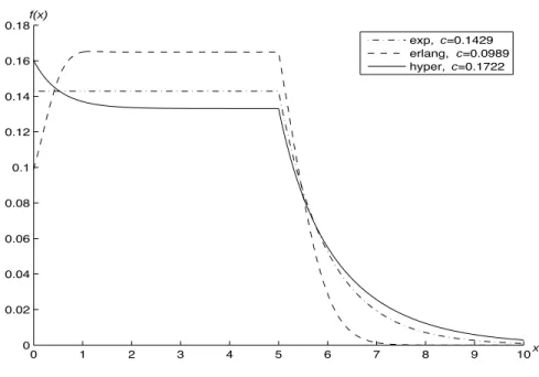
2.4 f(x) for different service time distributions, ρ= 1, b= 5 . . . 32

2.5 f(x) for different service time distributions, ρ= 1.2, b= 5 . . . 33

2.6 f(x) for different ρ, exponential service time, b= 5 . . . 33

2.7 W¯ vs. ρ for different service time distributions, b = 5 . . . 34

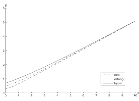
2.8 W¯ vs. b for different service time distributions, ρ= 0.8 . . . 34

2.9 W¯ vs. b for different service time distributions, ρ= 1 . . . 35

2.10 ¯W vs. b for different service time distributions, ρ= 1.2 . . . 35

2.11 cvs. λ for different service time distributions . . . 36

3.1 A Typical Sample Path ofXr(t) . . . 45

3.2 Construction ofW(t) . . . 51

3.3 Construction ofXr(t) . . . 51

3.4 Mean Plot,b = 2, ρ= 0.8 . . . 58

3.5 Mean Plot,b = 2, ρ= 1 . . . 58

3.6 Mean Plot,b = 2, ρ= 1.2 . . . 59

3.7 Mean Plot, Exponential Service Time,b = 2 . . . 59

3.8 Distribution Plot,b = 2, ρ= 0.8 (two sets of three curves for x=1 and x=2) . . . 60

3.9 Distribution Plot,b = 2, ρ= 1 (two sets of three curves for x=1 and x=2) . . . 60

3.10 Distribution Plot, b = 2, ρ= 1.2 (two sets of three curves for x=1 and x=2) . . . 61

3.11 Distribution Plot, Erlang Service Time, b= 2, x= 1 . . . 61

3.13 Density Plot, b = 2, ρ= 0.8, (two sets of three curves

for x=1 and x=2) . . . 62

3.14 Density Plot, b = 2, ρ= 1 (two sets of three curves for x=1 and x=2) . . . 63

3.15 Density Plot, b = 2, ρ= 1.2 (two sets of three curves for x=1 and x=2) . . . 63

3.16 Density Plot, Erlang Service Time, b= 2, x= 1 . . . 64

3.17 Density Plot, Erlang Service Time, b= 2, ρ= 0.8 . . . 64

3.18 Mean Plot, Exponential Service Time, ρ= 0.8 . . . 65

4.1 A sample path ofW(t) andN(t) . . . 68

4.2 Long-run Average Queueing Time for All Served Customers . . . 90

4.3 Fraction of Rejected Customers . . . 90

4.4 Relative Errors of Approximations: s = 3 . . . 91

4.5 Relative Errors of Approximations: s = 10 . . . 91

Chapter 1

Introduction

1.1

Overview

A significant aspect in modeling call centers is customer impatience (cf. Koole and Mandelbaum [27], Garnett et al. [15], Whitt [48]). Motivated by analyzing the call center operations, we consider anM/G/squeueing system with impatient customers. The customers arrive according to a Poisson process with rate λ, and request iid (independent and identically distributed) service times with a general distribution. There ares≥1 servers in the system available to serve the customers. All servers are identical and unit-rate, i.e., each server is capable of processing one unit of service requirement per unit time.

getting served if the wait in line becomes too long. This is the reneging behavior. Of course, there can be a combination of the two.

Queueing models with balking incorporate the characteristics of the customers’ impatience or a specific admission control policy in force at a service system. In a typical queueing model with balking the service requirement of an arriving customer may not be (completely) accepted if the system is “too congested” at the time of its arrival. From the perspective of an arriving customer one natural measurement of system congestion is the queueing time he/she faces to get service started. A no-join decision based on this congestion measurement is the aforementioned wait-based balking. The model considered in this thesis uses a wait-based balking rule. Before stating the balking rule, we define thevirtual queueing time (vqt) in the system. The vqt at timetin the system, denoted by W(t), is the queueing time (i.e., time spent in the system before commencing service) that would be experienced if a customer joins the system at timet. The process{W(t), t≥0} is referred as vqt process. We call a queueing system with balking based on the vqt a wait-based balking queue. It works as follows. We assume that each customer knows his/her exact queueing time at the time of arrival. A customer arriving at time t joins the system if and only if W(t−) is no more than a pre-specified threshold (possibly random). The balking customers (i.e., customers who do not join) are lost forever. The entering customers wait in an infinite capacity FCFS (first-come, first-served) queue until a server is available and leave when the service completes.

policy based on the system workload. Such a policy is shown to be optimal under certain conditions by Johansen and Stidham [25]. This threshold type policy gener-ates the model considered here. The usefulness of the wait-based balking model for studying reneging systems will become clear in Chapter 4, where we reveal a close relation between two models.

not depend on the number in the system, then the exact analysis of such models can be done using the methods developed here.

The vqt process is also known as work-in-system, or virtual-delay process, which is introduced by Beneˇs [6] and Tak´acs [44]. See Heyman and Sobel [19] (pages 383–390) for details. Many system performance measures of the queue can be derived from the steady state distribution of the vqt process. The central topic of this thesis is the steady state analysis of this process in several particular wait-based balking queues.

1.2

Single Sever Queues

Single server wait-based balking queues are studied under a variety of names in the literature: “finite workload capacity”, “dams”, “workload-dependent arrival rates”, or “queues with limited accessibility”. See Prabhu [42], Perry et al. [41], Perry and Stadje [39], Bekker et al. [5] and Bekker [4]. Wait-based balking queues also have found applications in the study of clearing models, see Boxma et al. [9].

Notice for single server systems with a FCFS service discipline, the vqt coincides with the workload (work content) of the system, i.e., sum of the service times of all customs in queue and the remaining service time of the customer in service (see page 10 for an alternative definition). Therefore, we use two terms interchangeably in the single server context.

1.2.1

Steady State Distribution

In Chapter 2 we deal with the steady state distribution of the workload process in the M/G/1 queue with wait-based balking.

sys-tem with workload restrictions in terms of that of the corresponding queue without restrictions. This requires the unrestricted system to be stable so as to solve the restricted system. But clearly the system with workload restriction is always stable. The inability to solve the restricted system when the corresponding unrestricted sys-tem is unstable is inevitable due to the “cut and paste” technique they use, since the basic idea of such a method is to obtain the steady state distribution of the limited access queueing models in terms of known steady state distribution of simpler models with no access constraints.

Level-crossing argument is an appropriate tool to analyze such queueing models. Cohen [11] introduces Level-Crossing Theory (LCT) for regenerative processes of the GI/G/1 type. Doshi [13] generalizes the theory to stationary dam process and presents applications of level-crossing analysis to many queueing systems, especially to single-server queues. Gavish and Schweitzer [16] use level-crossing analysis to study an M/G/1 system where arrivals are rejected if their queueing plus service times would exceed a fixed amount (note that the service time for each customer is known upon arrival, which is different from the wait-based balking queue we consider here). Hokstad [22] uses the method of level crossing method and computes explicitly the steady state distribution in the M/D/1 queue with wait-based balking. Perry and Asmussen [38] deal with the most general type of single server wait-based balking models with several variations. They develop the integral equation for the steady state distribution of the workload. The solution is given in terms of an infinite sum of iterated convolution integrals. The authors give explicit solution for the M/M/1 queue, and mention that explicit solutions can be obtained for M/P H/1 queues, but do not give the expressions. We have been unable to find the explicit expressions in the literature.

general distributions and we solve the equation explicitly for several special cases of service time distributions, such as phase type, Erlang, exponential and deterministic service times. For the M/P H/1 case we show that the integral equation can be reduced to a differential equation with constant coefficients, and hence can be solved by standard methods. We illustrate the results with several numerical examples.In Chapter 2, we use level-crossing argument to derive an integral equation for the steady state workload distribution. We describe a procedure to solve the equation for general distributions and we solve the equation explicitly for several special cases of service time distributions, such as phase type, Erlang, exponential and deterministic service times. For theM/P H/1 case we show that the integral equation can be reduced to a differential equation with constant coefficients, and hence can be solved by standard methods. We illustrate the results with several numerical examples.

1.2.2

Busy Period

The busy period is the first passage time that the vqt process enters the state 0. There are relatively few papers studying the busy period of the wait-based balking systems. Perry and Asmussen [38] find the LST of the busy period for the M/M/1 system via differential equations and martingales. They further extend the results to the case where b is an exponential random variable. Perry et al. [40] give closed-form expression for the LST of the busy period for anM/G/1 queue with wait-based balking as a function of the LSTs of certain stopping times. The paper also analyzes the busy periods inG/M/1 queues by exploiting the duality between theM/G/1 and G/M/1 queues.

paper by Kulkarni [30]. Various authors have studied the first passage times in fluid models. See Asmussen and Bladt [3], Chen and Samalam [10], Kulkarni and Narayanan [31], Boxma and Dumas [8] and Kulkarni and Tzenova [32]. In particular, Kulkarni and Tzenova [32] developed a differential equation method which is more suitable for numerical algorithms. We extend the method and use it to solve the first passage time problem arising in wait-based balking queues. In Chapter 3 we begin by considering a fluid model where the buffer content changes at a rate determined by an external stochastic process with finite state space. We derive systems of first-order linear different equations for both the mean and LST (Laplace-Stieltjes Transform) of the busy period in this model and solve explicitly. We obtain the mean and LST of the busy period in the M/P H/1 queue with wait-based balking as a special limiting case of this fluid model. We illustrate the results with numerical examples.

1.3

Multi-Server Queues

In Chapter 4 we extend the method used in the single server case to the analysis of the multi-server case.

heuristic for the M/G/s case. A severe restriction is that the formula is valid only when the traffic intensity is less than 1, which is not required for the reneging queue to be stable. The method we use in this thesis overcomes the preceding drawbacks and can be easily extended to the general case. Although we are unable to give the joint distribution for the workload and busy servers, we don’t lose much since many common performance measures can be derived directly from the limiting distribution of the vqt process.

Even in the absence of the balking behavior the M/G/s queueing system is no-torious for its complexity which forbids analytical solutions. Analytical results are available for only a few special cases, while a handful of approximations for the lim-iting analysis have been proposed in the past decades (cf. Chapter 13, Heyman and Sobel [19]). In this thesis we focus on system approximations, i.e. approximations that take the results from an exact analysis of a simpler system as approximations of the true operating characteristics of the original system. Although the approximate methods vary by motivations and the techniques used, it turns out that all results can be viewed as the so-called “systems interpolation”, i.e., some mixture of the known analytical results for a few special cases, such as M/M/s, M/Ek/s, M/D/s, and M/G/∞. See Kimura [26] for details. We cannot find any system approximations of

the M/G/s queueing system with impatient customers in the literature.

Chapter 2

M/G/

1

Queues with Wait-based

Balking: Steady State

Distributions

2.1

Introduction

In this chapter, we analyze a single server first-come first-served (FCFS) wait-based balking system that operates as follows: an arriving customer joins the queue only if he/she sees that the workload in the system is no more than a fixed amount b. We assume the customer knows the exact amount of the workload in the system at the time of arrival. We also assume that once a customer decides to join the queue, he/she stays in the system until service completion.

than b unit of time for start of service.

The assumption of FCFS discipline is not necessary if we do not require vqt to be the same as workload. The analysis in this chapter proceeds identically without this assumption since in general, the workload process is invariant under work-conserving service disciplines. Here we assume FCFS in which case the work content also repre-sents the queuing time, and hence the model reprerepre-sents customers balking in face of long waits.

The rest of this chapter is organized as follows. Section 2.2 is a description of the model. In Section 2.3, level-crossing argument is used to derived the integral equation for the steady state distribution of the workload process. Section 2.4 deals with the case when service time distribution has a rational Laplace transform (LT). In particu-lar, if the service time has a phase type distribution, we show a method to reduce the integral equation to a differential equation that can be solved by standard methods and give explicit formulas for probability distribution and selected performance mea-sures. Special cases, namely, exponential, phase type and hyper exponential service time distributions are included. Section 2.5 deals with the M/D/1 case. We give several numerical examples in Section 2.6. The chapter is concluded with a comment on other performance measures and balking rules (Section 2.7).

2.2

An

M/G/1

Queue with Balking

We begin with an M/G/1 system with Poisson arrivals with rate λ, and iid service times. Let S be a generic service time random variable, and

Pr{S > x}=G(x), E(S) =τ, Var(S) = σ2. (2.1)

Thus, the traffic intensity is

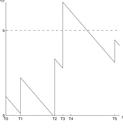
Let{W(t), t≥0}be the workload or vqt process. The balking rule is characterized by a constant b <∞as follows: A customer arriving at time t joins the system (and stays until service completion) ifW(t−)≤b, else he/she leaves and is lost. A typical sample path of W(t) is shown in Figure 2.1. The arriving times are denoted by Ti. Note that the arrival at T4 balks sinceW(T4−)> b.

T0 T1 T2 T3 T4 T5

0 b

t W(t)

Figure 2.1: A typical sample path of W(t)

It is known that the{W(t), t≥0}process has a limiting distribution ifE(S)<∞ (cf. [38]), which we will assume in this thesis. Let

F(x) = lim

t→∞Pr{W(t)≤x},

¯

W = lim

for x >0. We focus on computing c, f(x)(x≥0) andF(x)(x≥0).

2.3

Equilibrium Distribution of Workload Process

In this section, we derive the equation for f(x) and c in Theorem 1. We describe a procedure to find the solution in Theorem 2. We also discuss several limiting cases of parameters b and ρ.

Theorem 1. The equilibrium probability density function (pdf ) of the workload

pro-cess of the M/G/1 queue with balking satisfies:

f(x) = λ

Z x∧b

0

f(u)G(x−u)du+cλG(x), (2.3a)

Z ∞

0

f(x)dx+c= 1, (2.3b)

where x∧b = min(x, b).

Proof. We prove this by level-crossing argument. Suppose the process {W(t), t≥0} is stationary. Then, during interval (t, t+ h), the probability that the workload down-crosses level x is:

[F(x+h)−F(x)](1−λh). (2.4)

Thus this is also the expected number of down-crossings during (t, t+h). Similarly, the probability that the workload up-crosses level x is:

Z x∧b

0

f(u)λhPr{S ≥x−u}du+ Pr{W(∞) = 0}λhPr{S ≥x}, (2.5)

which, using our notations yields

Z x∧b

0

Thus this is also the expected number of up-crossings during (t, t+h).

The level-crossing argument implies that (2.4) must equal to (2.6) (cf. [13]). Now divide both side byh and let h→0. We get Equation (2.3a). Equation (2.3b) is the normalizing equation.

Notice that the first term in the right hand side of Equation (2.3a) is just the convolution off(x) andG(x) multiplied byλ, when x∧b is replaced byx. Let f1(x)

be the solution to

f1(x) =λ

Z x

0

f1(u)G(x−u)du+G(x), x≥0. (2.7)

Let

f2(x) =λ

Z b

0

f1(u)G(x−u)du+G(x), x≥b (2.8)

The solution to Equation (2.3) is given in the following theorem.

Theorem 2. The solution to (2.3) is:

f(x) =



 

 

cλf1(x) if 0≤x≤b

cλf2(x) if x > b

(2.9)

where

c=

λ

Z b

0

f1(x)dx+λ

Z ∞

b

f2(x)dx+ 1

−1

. (2.10)

Proof. The solution is easy to verify by substitution.

From the above theorem it is clear that a possible procedure to obtain f(x) is to find f1(x) first, then compute f2(x) by using Equation (2.8). By the normalizing

Let G∗(s) be the LT of G(x). From (2.7) we get the LT of f1(x) (assuming its

existence):

f₁∗(s) = G

∗_(s)

1−λG∗_(s). (2.11)

To continue our procedure, we need the inverse LT of f₁∗(s). A close form inversion is possible if G∗(s) is rational. However, in this case, there is an alternative method to solve Equation (2.7). We demonstrate these in Section 2.4.

We can instantly obtain several interesting results from Theorem 2 under some limiting values of b and λ. The first case is b → 0. Under this regime, the system reduces to a normal M/G/1/1 queue. From Theorem 2, as b→0,

c→ 1

1 +ρ, (2.12)

f(x)→ λ

1 +ρG(x), x >0 (2.13) ¯

W → λ

2(1 +ρ)(σ

2_+τ2_{). (2.14)}

It is easy to verify that the results above coincide with the results of an M/G/1/1 queueing system.

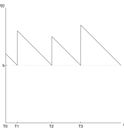
Next consider the limiting regimeλ→ ∞. A sample path of workload is illustrated in Figure 2.2. Obviously,

lim

T0 T1 T2 T3 b

t W(t)

Figure 2.2: A sample path of W(t) when λ→ ∞ Using the fact above we get

f(x)→0, when 0≤x≤b, (2.15) f(x)→ 1

τG(x−b), when x > b, (2.16)

c→0, (2.17)

¯

W →b+ 1 2τ(σ

2

+τ2). (2.18)

is stable for ρ <1. Notice that

Z ∞

0

f1(x)dx=f1∗(0),

G∗(0) =τ, ¯

W =− df

∗_(s)

ds

_s=0

.

From Theorem 2 and Equation (2.11), we get the following limiting results which are consistent with the usual M/G/1 results.

f(x)→cλf1(x), (2.19)

c→1−ρ, (2.20)

¯

W → λ(σ

2_+τ2₎

2(1−ρ) . (2.21)

In Section 2.4 and 2.5 we focus mainly on solving Equation (2.7) for several specific service time distributions by transform or directly.

2.4

Rational

G

(s)

and

M/P H/1

Queue with

Balk-ing

Suppose G∗(s) is rational, i.e.,

G∗(s) = N(s)

D(s), (2.22)

where D(s) is a pdegree polynomial in s, N(s) is a polynomial in s whose degree is less than p. Then

f∗(s) = N(s)

Letθi,i= 1,2,· · · , p, be the roots to

D(s)−λN(s) = 0. (2.24)

We assume they are distinct. Then from general method of computing inverse LT (cf. [28]), we obtain a closed form expression for f1(x) as follows:

f1(x) =

p

X

i=1

Aieθix, (2.25)

where

Ai = lim s→θi

(s−θi)G∗(s)

1−λG∗_(s) , i= 1,2,· · · , p. (2.26)

Next, as a specific example, we apply our method to solve the M/P H/1 case (which has a rational G∗(s)). In addition, we give results for Erlang, hyper exponential and exponential distributions as three more special cases of the phase type distribution.

2.4.1

M/P H/

1

: Transform Method

For a common phase type distribution with parameter (α, M) (cf. [29]), the comple-mentary cumulative distribution function (ccdf)G(x) is given by

G(x) =αeM x~1, (2.27)

where~1 is a column vector with all coordinates equal to 1, α = (α1, α2,· · · , αn) is a

non-negative row vector andα~1 = 1, andM is annbynsub-matrix of the generator of an irreducible CTMC (continuous time Markov chain), with the following properties:

• M is invertible;

It is well known that these properties imply that all eigenvalues of M have negative real part. We need this condition in the computation of f2(x). In this case the LT of

G(x) is

G∗(s) =α(sI −M)−1~1, (2.28)

where I is an n byn identity matrix.

Following the procedure described in Section 2.3, we collect our results for the M/P H/1 with wait-based balking in Theorem 3.

Theorem 3. Let the service time distribution be a common phase type distribution

with ccdf given by (2.27). The equilibrium pdf of the workload process of theM/P H/1

wait-based balking queue with threshold b is:

f(x) =

         cλ n X i=1

Aieθix if 0≤x≤b

cλα

eM x+ n

X

i=1

λAieM x(θiI−M)−1(e(θiI−M)b−I)

~_{1 if x > b} (2.29)

where θi, i= 1,2,· · · , n, are n distinct roots to Equation (2.24). Ai, i= 1,2,· · · , n,

are given by Equation (2.26), and G∗(s) is given by Equation (2.28). The probability that the system is empty is:

c=

n

X

i=1

λAi θi

(eθib₋₁₎

−αh n

X

i=1

λ2AiM−1eM b(θiI−M)−1(e(θiI−M)b−I)

i

~₁

−λαM−1eM b~1 + 1

−1

.

(2.30)

Proof. Use Equation 2.25 to take inverse LT of f₁∗(s) and apply Theorem 2.

A straight forward computation yields the following corollaries.

wait-based balking queue with threshold b is:

F(x) =

                      

c+cλ n

X

i=1

Ai

θi(e

θix−_{1), if 0}≤_x≤_b,

F(b) +cλαM−1(eM x−eM b) × I+ n X i=1

λAi(θiI−M)−1(e(θiI−M)b_−I)

~_{1, if x > b.}

Corollary 2 (Mean workload in equilibrium). The expected value of the workload in steady state of the M/P H/1 wait-based balking queue with threshold b is:

¯

W =b−bc−cλ n X i=1 Ai θ2 i

(eθib _−θ

ib−1)

+cλαM−2eM b

I+ n

X

i=1

λAi(θiI −M)−1(e(θiI−M)b _−I)

~_1.

Remarks:

1. If we write Equation (2.24) as 1−λα(sI−M)−1~1 = 0, it is easy to see that when ρ= 1, i.e.,−λαM−1_{~1 = 1, thenθ}

1 = 0 is one of the roots. In this case, we replace

the zero-dividing terms which appear in our results by the limits. These terms and the limits are: limθ1→0(e

θ1b−1)/θ

1 =band limθ1→0(e

θ1b−θ

1b−1)/θ21 =b2/2.

Therefore, we do not give the results separately for the case whenρ= 1.

2. Computing cneeds the integralR_b∞eM x to converge. This is guaranteed by the aforementioned fact that all eigenvalues of M have negative real part.

3. Notice that

E(S) =−αM−1_{~1 = τ, (2.31)}

It can be verified that the formulas above for limiting parameters b and ρ are consistent with those given for general service time distribution in Section 2.3. This is also illustrated by numerical examples in Section 2.6.

2.4.2

M/P H/

1

: Differential Equation Approach

In practice it can be hard to compute G∗(s), i.e., specifying the polynomials, for a general phase type distribution. Therefore, we seek an alternative way to solve Equation (2.7) directly. In order to solve for f(x), we first solve the integral equation (2.3a) for the case x≤bby solving a derived differential equation. Then we compute f(x) for the casex > bby the integral equation. We describe the method in Theorem 4.

First we introduce some notations that will be used in the statement and proof of Theorem 4.

Let ai, i = 0,1,· · · , n, be the coefficients of the characteristic polynomial of M, i.e. :

det(xI−M) = n

X

j=0

ajxj. (2.33)

Let

P(θ) = n

X

i=0

αaiI+λ i

X

j=0

ajMj−i−1

~₁

θi (2.34)

be an n-th order polynomial in θ. We assume P(θ) has n distinct roots. Note that if −αM−1_{~1 = 1/λ (i.e. traffic density ρ=−λαM}−1_{~1 = 1), then θ}

1 = 0 is one of the

roots.

Let M0 =I, and defineMj, j ≥1 recursively by:

Let

mi =αMi~1, i= 0,1,· · · , n−1 and m= (m0, m1,· · · , mn−1)T.

(2.36)

With these notations, we are ready to state the following theorem.

Theorem 4. The constants θi, i = 1,2,· · · , n, in Theorem 3 are the roots of P(θ)

given in (2.34). The coefficient A = (A1, A2,· · · , An)T is uniquely determined by:

ΘA=m, (2.37)

where Θis the Vandermonde matrix of θ1, θ2,· · · , θn, i.e.:

Θ =            

1 1 · · · 1

θ1 θ2 · · · θn θ2

1 θ22 · · · θn2

..

. ... . .. ...

θ₁n−1 θn₂−1 · · · θn_n−1

            .

Proof. Plugging (2.27) in Equation (2.7) and simplifying, we get:

f1(x) =λαeM x

Z x

0

f1(u)e−M udu+I/λ

~_{1. (2.38)}

f₁(i)(x) to denote the i-th order derivative of f1(x) with respect to x):

f₁(0)(x) = λαhM0_eM x

Z x

0

f1(u)e−M udu+I/λ

i

~_1, f₁(1)(x) = λαhM1eM x

Z x

0

f1(u)e−M udu+I/λ

+f₁(0)(x)Ii~1, f₁(2)(x) = λαhM2_eM x

Z x

0

f1(u)e−M udu+I/λ

+M f₁(0)(x) +f₁(1)(x)Ii~1, ..

.

f₁(n)(x) = λαhMn_eM x

Z x

0

f1(u)e−M udu+I/λ

+ n−1

X

j=0

Mj_f(n−1−j)

1 (x)

i

~_1.

(2.39) Now multiply thei-th equation above by coefficientaiin the characteristic polynomial of M as defined in (2.33) and add. We get:

n

X

i=0

aif

(i)

1 (x) =λα

h_Xn

i=0

aiMieM x

Z x

0

f1(u)e−M udu+I/λ

+ n

X

i=0

i−1

X

j=0

aiMjf

(i−1−j) 1 (x)

i

~_1. (2.40) By Cayley-Hamilton Theorem, we know

n

X

i=0

aiMi = 0. (2.41)

Using this and doing algebraic manipulations, Equation (2.40) can be simplified and rewritten as:

n

X

i=0

αaiI+λ i

X

j=0

ajMj−i−1

~₁

f₁(i)(x) = 0. (2.42)

This is simply an n-th order differential equation with constant coefficients. Using standard methods of solving such equations (cf. [28]), we get the polynomial (2.34) and the solution f1(x) =

Pn

The initial conditions can be found by plugging x= 0 in (2.39):

lim x→0f

(j)

1 (x) =mj, j = 0,1,· · · , n−1, (2.43)

where mj are as defined in (2.36). This yields (2.37). Since all θi are distinct by assumption, Θ is invertible (cf. [20]) thus A is uniquely determined.

2.4.3

Special Cases

Next, we consider three special cases of service time distribution: Erlang, hyper-exponential and hyper-exponential. These belong to the common phase type distribution category, and have special parameters (α, M). For these cases we can, more or less, simplify the results for a general phase type distribution.

Erlang

An Erlang distribution with parameter (n, µ) is simply a phase type distribution with parameter:

α= (1,0,· · ·,0)1×n,

M =             −µ µ −µ µ . .. ... −µ µ −µ            

n×n

(We display only the non-zero entries ofM).

We solve f1(x) by transform. Using Equation (2.28), G∗(s) can be shown to be

G∗(s) = (s+µ) n_−µn

Finding the roots to 1−λG∗(s) is equivalent to solving the following equation:

1

s[(s−λ)(s+µ) n

+λµn] = 0. (2.45)

Note that the left hand side is actually ann degree polynomial ins. It can be proved that there are exactly n distinct roots, θ1, θ2,· · · , θn. So, writingf1∗(s) as

f₁∗(s) = G

∗_(s)

1−λG∗_(s)

=

1

s[(s+µ)

n_−µn_]

1

s[(s−λ)(s+µ)n+λµn] = (s−λ)

−1_[Qn

i=1(s−θi)−

Qn

i=1(λ−θi)]

Qn

i=1(s−θi)

,

(2.46)

then computing Ai by Equation (2.26) yields

Ai =

Y

j6=i

λ−θj θi−θj

, i= 1,2,· · · , n.

Next, we compute the matrix exponential explicitly and give the result in Theorem 5. Before that, we introduce two more notations. We denote the well known incomplete gamma function by:

Γ(n, x) =

Z ∞

x

tn−1e−tdt = (n−1)!e−x n−1

X

k=0

xk k!.

Let

di = µ µ+θi

, i= 1,2,· · · , n.

Theorem 5. The equilibrium pdf of the workload process of the M/En/1 wait-based

balking queue with threshold b is:

f(x) =cλ n

X

i=1

and

f(x) = cλ2 n

X

i=1

Ai θi(n−1)!

dn_ieθix_{Γ n,(µ+θi)x−Γ n,(µ+θi)(x−b)}

+eθib_{Γ n, µ(x−b)−Γ(n, µx)}

+cλΓ(n, µx)

(n−1)!, if x > b.

c−1 =λ n

X

i=1

Ai θi

(eθib_{−1) +} λ

µ(n−1)![Γ(n+ 1, µb)−µbΓ(n, µb)] + 1 +λ2

n

X

i=1

Ai µθ2

i(n−1)!

{µ(1 +θib)Γ(n, µb)−µdnie

θib_{Γ n,(µ+θ}

i)b

−θiΓ(n+ 1, µb) +θieθibn!−µeθib(1−dni)(n−1)!}

Hyper-exponential

If the service time S has a hyper-exponential distribution (cf. [29]), then

α= (α1, α2,· · · , αn)T,

M =       −µ1 . .. −µn       .

In this case, f1(x) can be solved either by transform or directly. Here we only show

some results by using Theorem 4 to solve f1(x) directly.

The characteristic polynomial of M is: n

X

i=0

aixi = n

Y

i=1

(x+µi).

Equation (2.34) in terms of the moments of S as follows:

P(θ) = n

X

i=0

biθi,

where

bi =ai+λ i+1

X

j=1

ai+1−j(−1)j E(Sj)

j! .

Unfortunately, the initial conditions do not simplify, hence we keep the remaining results in terms of m of (2.36) and A of (2.37).

Exponential

Exponential distribution is the most special case of phase type distribution. It is also a special case of Erlang or hyper-exponential distributions. All matrices and vectors we use in a common phase type distribution degenerate to scalars in an exponential distribution. The parameters are simply α = (1) and M = (−µ). Using either transform of direct method, the formulas are much simplified.

We give the simplified solution in the following theorem and skip the proof.

Theorem 6. The equilibrium pdf of the workload process of the M/M/1 wait-based

balking queue with threshold b is:

f(x) =



 

 

cλe−(µ−λ)x if 0≤x≤b cλeλbe−µx if x > b

,

where

c=



 

 

1−ρ

1−ρ2_e−(µ−λ)b if ρ6= 1

1

2.5

An Example of Non-rational

G

(s)

:

M/D/1

As we mentioned before, it can be difficult to find the inverse LT off₁∗(s) whenG∗(s) is not rational. In this case, we try to solve Equation (2.7) directly. Here we give the solution when the service time is deterministic, i.e.,

G(x) =



 

 

1 if 0≤x < τ 0 if x≥τ

(2.47)

In this case, the LT of f1 is given by

f₁∗(s) = 1−e sτ

s−λ+λe−sτ. (2.48)

Computing its inverse is intractable. We show how we solve (2.7) directly in this case. First we partition [0,+∞) into intervals of length τ: [0, τ),[τ,2τ),· · · and denote them as I0, I1,· · · respectively. Since G(x) is 1 when x ∈ I0 (or bx_τc = 0) and 0

elsewhere, we rewrite Equation (2.7) as follows:

λ

Z x

0

f1(u)du+ 1 =f1(x), whenx∈I0,

λ

Z kτ

x−τ

f1(u)du+λ

Z x

kτ

f1(u)du=f1(x), whenx∈Ik, k= 1,2,· · ·.

(2.49)

We solve these equations recursively and obtain f1(x) for each interval. That is, we

solve the first equation and get f1(x) = eλx when x∈I0. Plugging this in the second

equation, we are able solve for f1(x) when x∈I1, and so on. Suppose

f1(x) = Qk(x)eλ(x−kτ), when x∈Ik, k = 0,1,2,· · ·, (2.50)

take derivative with respect to x, we get

Q0_k(x) = −λQk−1(x−τ), k= 1,2,· · · . (2.51)

Therefore,Qk(x) can be computed recursively as

Qk(x) =−λ

Z x

0

Qk−1(u−τ)du+Bk, k = 1,2,· · · . (2.52)

The constantBk can be computed by the fact thatf1(τ−) = f1(τ+) + 1 andf1(x) is

continuous at 2τ,3τ,· · ·. We get

B1 =eρ+ρ−1,

Bk=Qk−1(kτ)eρ+λ

Z kτ

0

Qk−1(u−τ)du, k = 2,3,· · · .

In the special case whenb < τ, the computation is fairly easy. We give the results here.

f(x) =



       

       

cλeλx _{if 0≤x≤b} cλeλb _{if b < x < τ} cλ(eλb_−eλ(x−τ)_{) if τ ≤x < b+τ}

0 elsewhere

(2.53)

In this case the probability that the system is empty is

c= 1

τ λeλb_{+ 1}. (2.54)

2.6

Numerical Examples

1. Exponential (exp): µ= 1 (τ = 1, σ2 = 1);

2. 5-Erlang (erlang): µ= 5 (τ = 1, σ2 = 0.2);

3. Hyper-exponential (hyper): µ1 = 4, µ2 = 2, µ3 = 1, µ4 = 0.8, µ5 = 0.5, α1 =

· · ·=α5 = 0.2 (τ = 1, σ2 = 1.75).

All of them have mean service time of one. The variances are different, with 5-Erlang the smallest and hyper-exponential the largest.

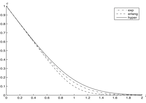
The first set of figures, Figure 2.3, 2.4, 2.5 illustrate the shapes off(x) for different service time distributions, with ρ= 0.8,1,1.2 respectively and b = 5. Then, we pick curves for exponential service time from Figure 2.3, 2.4, 2.5 and put them together in Figure 2.6 to show how f(x) is affected by the traffic intensity. As ρ gets larger, the turn at x=b becomes sharper. When ρ1 (in our experiment, ρ= 10 is large enough), f(x) is almost 0 when x < b. Note that f(x) is a decreasing function of x forx > b. However, for 0< x < b, the density function can exhibit complex behavior. It may be increasing, decreasing, constant or non-monotonic.

The second set of figures, Figure 2.7, 2.8, 2.9 and 2.10, are about the expected workload in steady state ( ¯W). In Figure 2.7, we fix b = 5 and compare ¯W for dif-ferent service time distributions against ρ (since τ = 1, ρ =λ). When ρ gets larger,

¯

W clearly converges to the levels as expected (see Equation (2.18)), to be specific, to 6, 5.6 and 6.375 for exponential, Erlang and hyper-exponential distributions, respec-tively.

Finally, Figure 2.11 shows the probability that the system is empty in steady state. As expected, cis decreasing in arrival rate λ.

2.7

Concluding Remarks

It is possible to extend the method used in this chapter to handle more complicated cases, e.g., models with load dependent service rates and vacations, or random balking threshold. We do not cover those in order to emphasize a basic idea by relatively simple models.

Although we focus on the steady state distribution of the workload process in this chapter, typically several other system performance measures are of interest. For example, the steady state rejection rate can be easily computed as 1−F(b), where F is the steady state cdf of the vqt process. Secondly, the expected busy period can be computed from the standard regenerative analysis as (1−c)/(λc), where c is the probability that the workload is zero in steady state. Similarly, the expected number in the system can be computed by using Little’s law. However, the distribution of the busy period would require further analysis. We shall study this topic in Chapter 3. Also, since we have computed the steady state distribution of the workload, the expected values of its functionals are easy to compute.

0 1 2 3 4 5 6 7 8 9 10 0

0.05 0.1 0.15 0.2 0.25 0.3 0.35

x f(x)

exp, c=0.2616 erlang, c=0.2266 hyper, c=0.2874

Figure 2.3: f(x) for different service time distributions,ρ= 0.8, b = 5

0 1 2 3 4 5 6 7 8 9 10

0 0.02 0.04 0.06 0.08 0.1 0.12 0.14 0.16 0.18

x f(x)

exp, c=0.1429 erlang, c=0.0989 hyper, c=0.1722

0 1 2 3 4 5 6 7 8 9 10 0

0.05 0.1 0.15 0.2 0.25 0.3 0.35

x f(x)

exp, c=0.0686 erlang, c=0.0341 hyper, c=0.0938

Figure 2.5: f(x) for different service time distributions,ρ= 1.2, b = 5

[ I[

嘑 :

Figure 2.7: ¯W vs. ρ for different service time distributions, b= 5

嘑 :

嘑 :

Figure 2.9: ¯W vs. b for different service time distributions,ρ= 1

嘑 :

0 0.2 0.4 0.6 0.8 1 1.2 1.4 1.6 1.8 2 0

0.1 0.2 0.3 0.4 0.5 0.6 0.7 0.8 0.9 1

!

c

exp erlang hyper

Chapter 3

M/P H/

1

Queues with Wait-based

Balking: Busy Period Analysis

3.1

Introduction

Consider the M/P H/1 wait-based balking queue with a fixed balking thresholdb, as described in Chapter 2 (see page 18 for phase type distribution).

In this chapter, we are interested in the first passage time

B = min{t ≥0 :W(t) = 0}.

Specifically, we compute the mean

m(x) = E[B|W(0) =x] (3.1)

and the LST

ψ(s, x) = E[e−sB|W(0) =x]. (3.2)

[32] studied the first passage times in fluid models. They developed a differential equation method which is more suitable for numerical algorithms. We slightly extend the method so that it can be applied to the fluid model we construct, and obtain the mean and LST of the first passage time. The precise formulation of our fluid model is given in Section 3.2.

The rest of the chapter is organized as follows. We formulate the relevant fluid model in Section 3.2 and give a general treatment of the first passage time problem for this fluid model in Section 3.3. In Section 3.4, we consider a special case of the fluid model and give the mean and LST in Theorems 10 and 11. In Section 3.5 we show that the balking model is a limiting case of the fluid model analyzed in Section 3.4. Then we take the limits of the results given in Theorems 10 and 11 and obtain explicit formulas for the mean and LST of the first passage time for the balking model in Theorems 12 and 13. In Section 3.6, we illustrate the usage of these formulas to compute the first passage time in the M/M/1 case and verify several known results. We present several numerical examples in Section 3.7.

3.2

The Fluid Model

Consider a fluid model with an infinite capacity buffer where the net flow rate is gov-erned by a stochastic process{Z(t), t≥0}with a finite state space S ={0,1,· · · , n} as follows: if Z(t) = i the buffer level changes at rate ri. For convenience, we as-sume that ri 6= 0,∀i ∈ S. It will be clear later that this assumption is not a severe restriction in the context of our application. LetS− ={i:ri <0}, S+={i:ri >0},

n− =|S−| and n+=|S+|.

buffer content process X ={X(t), t ≥0} is given by:

dX(t) dt =



 

 

ri if Z(t) = i, X(t)>0, max(ri,0) if Z(t) = i, X(t) = 0.

TheXprocess is called afluid input-output process driven by theZ process(cf. Kulka-rni [30]). The driving process Z behaves as a CTMC whose infinitesimal generator matrix Q(x) depends on the current buffer levelx as follows:

Q(x) =



 

 

Q if 0≤x≤b, ¯

Q if x > b,

where Q = [qij] ( ¯Q = [¯qij]) is the generator of a CTMC. We assume that Q and ¯Q have exactly one irreducible class. Such CTMCs have unique limiting distributions that are independent of their initial states.

A more general version of a such a model is studied by Scheinhardt et al. [43] under the name “feedback fluid queue”.

Clearly the joint process {(X(t), Z(t)), t ≥0} is a Markov process which is char-acterized by the matrices Q, ¯Q and R = diag(r0, r1,· · · , rn). Let p = [p0, p1,· · · , pn] be the solution to

pQ= 0, p~1 = 1

and ¯p= [¯p0,p¯1,· · · ,p¯n] be the solution to

¯

pQ¯ = 0, p~¯1 = 1.

Let

d=X i∈S

and

¯ d=X

i∈S

¯ piri.

It is easy to see that ¯d <0 is a sufficient condition for the joint process to be stable ( Kulkarni [30]). We assume this condition holds, i.e., the joint process is stable.

3.3

First Passage Time: the Fluid Model

In this section, we compute the mean and LST of the first passage time

T = min{t ≥0 :X(t) = 0}.

Let

πi(x) = E[T|Z(0) =i, X(0) =x]

and denote

π(x) = [π0(x), π1(x),· · · , πn(x)]T.

Theorem 7. The vector π(x) satisfies the following system of differential equations

Rπ0(x) =



 

 

−~1−Qπ(x), if 0< x < b,

−~1−Qπ(x),¯ if x > b,

(3.3)

with boundary conditions:

πi(0) = 0, i∈ S−,

π(b−) = π(b+).

(3.4)

Proof. For 0< x < b, consider an infinitesimal time interval [0, h] and use first step analysis to obtain:

or

πi(x−rih) = h+ (1 +qiih)πi(x) +

X

j6=i

qijhπj(x), ∀i.

Divide both sides by h and leth↓0. After some algebra, we get:

−riπ0i(x) = 1 +

X

j

qijπj(x). (3.5)

The system of differential equations is obtained by rearranging the terms and writing the (n+ 1) equations in a matrix form. Same argument goes for the casex > b. The boundary conditions are obvious.

Notice that Equation (3.5) shows that it is possible to eliminate an unknownπj(x) if rj = 0. Hence assumingri 6= 0, ∀i∈ S is not a severe restriction.

Similar equations are derived and solved in Kulkarni and Tzenova [32] by using well-known techniques. We slightly extend the method that is used in Theorem 3.3 in Kulkarni and Tzenova [32] and apply it to the problem we consider here. First we state the following lemma.

Lemma 1. (From Theorem 11.5, Kulkarni [30]). Suppose Q¯ has exactly one irre-ducible class. Then there are n+ 1 (possibly repeated) eigenvalues of −R−1_{Q¯. When}

¯

d <0, exactly n+ have positive real parts, one is zero, and n−−1 have negative real parts.

Order the eigenvalues ¯θi as follows:

Re(¯θ0)≤Re(¯θ1)≤ · · · ≤Re(¯θn−−2)≤Re(¯θn−−1) = 0< Re(¯θn−)≤ · · · ≤Re(¯θn).

Let ¯vi be the right eigenvector corresponding to eigenvalue ¯θi.

Similarly, we use the notation θi and vi (i = 0,1, ..., n), respectively, for the eigenvalues and right eigenvectors of −R−1_{Q. But we do not order θ}

We give the main result in the following theorem. The proof is similar to that of Theorem 3.3 in Kulkarni and Tzenova [32] and is omitted here.

Theorem 8. Let I be the (n+ 1)×(n+ 1) identity matrix. The solution to Equa-tion (3.3) and (3.4) is given by:

π(x) =



 

 

Pn

j=0ajvjeθjx− ~1x

d +c, if 0≤x≤b,

Pn−−1

j=0 a¯jv¯je

¯

θjx₋~1x

¯

d + ¯c, if x > b,

(3.6)

where cis any solution to the linear system

Qc= (R/d−I)~1,

¯

c is any solution to the linear system

¯

Q¯c= (R/d¯−I)~1,

and the coefficients {aj,0≤j ≤n} and {¯aj : 0≤j ≤n−−1} are obtained by using the boundary conditions given in Equation (3.4).

Next, we compute the LST of the first passage time T:

φi(s, x) = E[e−sT|Z(0) =i, X(0) =x].

Let

φ(s, x) = [φ0(s, x), φ1(s, x),· · · , φn(s, x)]T.

Theorem 9. The vector φ(s, x)satisfies the following system of differential equations

Rdφ(s, x)

dx =



 

 

(sI−Q)φ(s, x), if 0< x < b,

(sI−Q)φ(s, x),¯ if x > b,

(3.7)

with boundary conditions:

φi(s,0) = 1, i∈ S−,

φ(s, b−) = φ(s, b+).

(3.8)

Proof. For 0< x < b, consider an infinitesimal time interval [0, h] and use first step analysis to obtain:

φi(s, x) =e−sh(1 +qiih)φi(s, x+rih) +

X

j6=i

e−shqijhφj(s, x+rih), ∀i,

or

φi(s, x−rih) =e−sh(1 +qiih)φi(s, x) +

X

j6=i

e−shqijhφj(s, x), ∀i.

Divide both sides by h and leth↓0. After some algebra, we get:

−ri

dφi(s, x)

dx +sφi(s, x) =

X

j

qijφj(s, x), ∀i.

The system of differential equations is obtained by rearranging the terms and writing the (n+ 1) equations in a matrix form. Same argument goes for the casex > b. The boundary conditions are obvious.

3.4

A Special Case of the Fluid Model

In this section we consider a special case of the fluid model whoseR,Qand ¯Qmatrices are as given below. As we shall see, this helps us solve the first passage time problem for the balking model we have described at the beginning of this chapter. Let M and α be the parameters of the phase type distribution as defined in Section 2.4.1 and λ be the arrival rate. The fluid model is parameterized by a real number r >0. Let

r0 =−1, ri =r >0 for i= 1,2,· · · , n, R= diag(r0, r1,· · · , rn),

(3.9)

Q=



 

−λ λα

−M r~1 M r





, (3.10)

¯ Q=



 

0 0

−M r~1 M r





. (3.11)

To understand the motivation behind this model consider two cases.

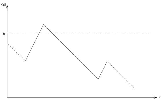
Case 1: The buffer content is no more thanb. Then the buffer content increases at rate r as long as the Z process is in the set {1,2, .., n} (we say it is “up”), and it decreases at rate 1 when the Z process is in state 0 (we say it is “down”). The Z process alternates between up and down periods. The down times are iid exp(λ) ran-dom variables, and the up times are iid with phase type distribution with parameters α and M.

Case 2: The buffer content is more than b. Then the buffer content increases at rate r as long as the Z process is up, and it decreases at rate 1 when the Z process is down. Once the Z process is down, it stays down until the buffer content drops below b and we switch to case 1 above.

parameters Q, Q, R¯ given above. A typical sample path of the {Xr(t), t ≥ 0} process is shown in Figure 3.1.

X_r(t)

t b

Figure 3.1: A Typical Sample Path of Xr(t)

Now define some special notation for this special case as follows:

Tr = min{t≥0 :Xr(t) = 0},

πi(x, r) = E[Tr|Z(0) =i, X(0) = x],

π(x, r) = [π0(x, r), π1(x, r),· · · , πn(x, r)]T,

φi(s, x, r) = E[e−sTr_{|Z(0) =i, X(0) =x],}

φ(s, x, r) = [φ0(s, x, r), φ1(s, x, r),· · · , φn(s, x, r)]T,

A(s, r) =R−1(sI−Q) =



 

−λ−s λα

M~1 −M +s_rI



and

¯

A(s, r) = R−1(sI−Q) =¯



 

−s 0

M~1 −M +s_rI



 .

First we give an explicit formula for the mean first passage time π(x, r) in the following theorem.

Theorem 10. With R, Q and Q¯ as specified in Equation (3.9), (3.10) and (3.11), respectively, the solution to Equation (3.3) and (3.4) is

π(x, r) =



 

 

eA(0,r)x_(c−Rx

0 e

−A(0,r)t_R−1_{~1dt), if 0≤x≤b,}

(x−b)~1 +π(b, r), if x > b,

where c=    u1

M~1,−M

eA(0,r)b



 

−1

 

0 (1 + 1/r)~1 +

M~1,−M

eA(0,r)bRb

0 e

−A(0,r)t_R−1_~1dt



 ,

and u1 is the first row of the identity matrix.

Proof. Substituting Qand ¯Q in Equation (3.3), we get:

dπ(x, r)

dx =−R

−1_~

1 +A(0, r)π(x, r), if 0< x < b, (3.12a) dπ(x, r)

dx =−R

−1_{~1 + ¯A(0, r)π(x, r), if x > b. (3.12b)}

It is well known (cf. Finizo and Ladas [14]) that the solution to Equation (3.12a) is

π(x, r) =eA(0,r)x(c−

Z x

0

e−A(0,r)tR−1~1dt), 0< x < b, (3.13)

Then

dπ(x, r)

dx =

d[(x−b)~1 +π(b, r)]

dx =~1, x > b. (3.14) Consider the value limx↓b

dπ(x,r)

dx . From Equation (3.14) and (3.12b), use the fact π(b−, r) = π(b+, r), we get:

−R−1_{~1 + ¯A(0, r)π(b−, r) =~1,}

which reduces to:

[M~1,−M]π(b−, r) = (1 + 1/r)~1.

Using Equation (3.13) for π(b−, r) we get:

[M~1,−M]eA(0,r)b(c−

Z b

0

e−A(0,r)tR−1~1dt) = (1 + 1/r)~1.

Sinceπ0(0, r) = 0, the first component ofcis 0. Writing this condition as an additional

row of the equation above, we get:



 

u1

M~1,−M

eA(0,r)b



 c=



 

0 (1 + 1/r)~1 +M~1,−M

eA(0,r)bRb

0 e

−A(0,r)t_R−1_~1dt



 .

Remark: Since A(0, r) is singular, it makes the computation of the integral

Rx

0 e

−A(0,r)t_{dttricky. There are several numerical methods for computing this integral.} The method we use in our computations is based on the following observation. Since π(x, r) = dφ(s,x,r_ds )|s=0, we have

Z x

0

e−A(0,r)tdt= lim s→0

Z x

0

e−A(s,r)tdt= lim s→0A

−1_{(s, r)(I−e}−A(s,r)x_).

First we need the following lemma.

Lemma 2. The matrix A(s, r)¯ has an eigenvalue −s with geometric multiplicity 1 and the corresponding right eigenvector:

¯ v0(r) =



 

1

(M −s(1 + 1/r)I)−1_M~1



 .

Proof. It is easy to verify that

(−sI −A(s, r))¯¯ v0(r) = 0,

and the null space of sI+ ¯A(s, r) has dimension 1.

The explicit formula for φ(s, x, r) is given in the following theorem.

Theorem 11. With R, Q and Q¯ as specified in Equation (3.9), (3.10) and (3.11), respectively, the solution to Equation (3.7) and (3.8) is

φ(s, x, r) =



 

 

eA(s,r)x_{c if 0≤x≤b,} e−s(x−b)_eA(s,r)b_{c if x > b,}

where

c=ke−A(s,r)b¯v0(r),

k is the scalar such that u1c= 1.

Proof. Substituting Qand ¯Q in Equation (3.3), we get:

dφ(s, x, r)

dx =A(s, r)φ(s, x, r), if 0< x < b, (3.15a) dφ(s, x, r)

It is well known that the solution to Equation (3.15a) is

φ(s, x, r) = eA(s,r)xc, 0< x < b, (3.16)

where cis some constant vector to be determined. Notice that for x > b

φi(s, x, r) = E[e−sTr|Z(0) =i, X(0) =x] = E[e−s(x−b+Tr)_{|Z(0) =i, X(0) =b]}

=e−s(x−b)φi(s, b, r).

Then

dφ(s, x, r)

dx =

d[e−s(x−b)_{φ(s, b, r)]}

dx =−se

−s(x−b)_{φ(s, b, r), x > b. (3.17)}

Consider limx↓b dφ(_ds,x,r_x ). From Equation (3.17) and (3.15b), using the factφ(s, b−, r) = φ(s, b+, r), we get:

¯

A(s, r)φ(s, b−, r) = −sφ(s, b−, r).

Using Equation (3.16) for φ(s, b−, r) we get

¯

A(s, r)eA(s,r)bc=−seA(s,r)b_c,

which implies thateA(s,r)bcis a right eigenvector of ¯A(s, r) corresponding to the eigen-value−s, i.e.:

eA(s,r)bc=k¯v0(r),

3.5

First Passage Time: the Balking Queueing Model

In this section, we compute the mean and LST of the first passage time for the balking queuing model. First we give the following construction which shows that the balking model is a limiting case of the fluid model we analyze in the previous section.

We construct the sample path of {W(t), t ≥ 0} in the balking model and the sample path of {Xr(t), t ≥ 0} in the fluid model on a common probability space as follows. Without loss of generality, assume the process{Xr(t), t≥0}start in “down” time.

Let {Ui, i≥1} be iid random variables with phase type distribution with param-eterα andM;{Di, i≥1}be iid random variables with exponential distribution with parameter λ. We think of Ui as the service time of the i-th arriving customer (who may or may not balk) andDi as the inter-arrival time between thei-th and (i+ 1)-st arriving customer. Then the sample path of the {W(t), t≥0} process in the balking model is completely described by these two sequences and the parameter b. It is shown in Figure 3.2. Note that the second customer (arriving at timeD1+D2) finds

the workload above b and hence balks.

Next we construct a sample path of the buffer content process {Xr(t), t ≥0} by using the same two sequences {Ui, i≥1} and {Di, i≥1}. It is shown in Figure 3.3. Here we use Di as the i-th down time, and Ui/r as the i-th up time. Note that if the i-th down time finishes while the buffer content is above b, we do not use the i-th uptime at all, and immediately start the next down time. This is equivalent to

having a null transition in the Z process from state 0 to 0. Such a transition occurs in Figure 3.3 at time D1+ U_r1 +D2.

Then, clearly,

{Xr(t), t≥0} a.s.

U₁

U 3

D₁ D₃

x W(t)

t

D₂ b

Figure 3.2: Construction ofW(t)

U

1 / r D2 U3 / r

D

1

U

3

U₁ x

X_r(t)

t b

D

3

Recall that B = min{t ≥ 0 : W(t) = 0} and Tr = min{t ≥ 0 : Xr(t) = 0}. It follows from the preceding construction that

Tr a.s. → B

as r→ ∞. Let

A(s) = lim

r→∞A(s, r) = 

 

−λ−s λα M~1 −M



 ,

¯

A(s) = lim r→∞

¯

A(s, r) =



 

−s 0

M~1 −M



 ,

and

¯

v0 = lim

r→∞¯v0(r) = 

 

1

(M −sI)−1M~1



 .

It is clear that if we take the limit of the results given in Theorem 10 and 11, then the first component of the vector is the first passage time for the balking model. We summarize the results in Theorems 12 and 13. The proof is straightforward and hence is omitted.

Theorem 12. The mean first passage time defined in Equation (3.1) is given by

m(x) =     

u1eA(0)x(c+

Rx

0 e

−A(0)t_uT

1dt), if 0≤x≤b,

(x−b) +m(b), if x > b,

where c=    u1

M~1,−M

eA(0)b



 

−1

 

0 ~₁₋

M~1,−M

eA(0)bRb

0 e

−A(0)t_uT 1dt



and u1 is the first row of the identity matrix.

Theorem 13. The LST of the first passage time defined in Equation (3.2) is given

by

ψ(s, x) =



 

 

u1eA(s)xc if 0≤x≤b,

u1e−s(x−b)eA(s)bc if x > b,

where

c=ke−A(s)bv¯0,

k is the scalar such that u1c= 1.

Remark: Differential equations similar to (3.3) and (3.7) also hold for other first passage times. For example, suppose T = min{t ≥ 0 : X(t) = 0 or X(t) = b}. This case is actually easier since the constant vector in the solution to Equation (3.3) is completely determined by the boundary conditions πi(0) = 0, i∈ S− and πi(b) = 0, i∈ S+. Similarly, the constant vector in the solution to Equation (3.7) is completely

determined by the boundary conditions φi(s,0) = 1, i∈ S− and φi(s, b) = 1, i∈ S+.

3.6

Special Case: Exponential Service Times

In this section, we illustrate the results of the previous section with exponential service time with rate µ, and verify the known results.

The exponential distribution is simply a phase type distribution with parameters:

M = [−µ], α= [1].

Thus we have

A(s) =



 

−s−λ λ

−µ µ   , ¯ A(s) =    0 0 −µ µ   ,¯v0 =



 

1 µ/(µ+s)



Using Theorem 12, after tedious algebra, we get the following result for the mean first passage times

m(x) =      1

(µ−λ)2[µ(µ−λ)x− λ 2

µe

−(µ−λ)(b−x)₊λ2 µe

−(µ−λ)b_{], if 0≤x≤b,}

(x−b) +m(b), if x > b,

. (3.18)

Equation 3.18 is equivalent to the formula given in Proposition 3.1 in Perry and Asmussen [38].

Using Theorem 13, after simplification, we get the following formula which is consistent with Theorem 3.1 in Perry and Asmussen [38]:

ψ(s, x) =

          

γ1eθ1x−γ2eθ2x

γ1−γ2 if 0≤x≤b,

e−s(x−b)ψ(s, b) if x > b,

(3.19)

where

θ1 =

(µ−s−λ) +p(s+λ−µ)2_{+ 4µs}

2 , (3.20)

θ2 =

(µ−s−λ)−p(s+λ−µ)2_{+ 4µs}

2 , (3.21)

are the eigenvalues of A(s) and

γi = (µ−θi − λµ s+µ)e

−θib_{, i= 1,2.}

From Equation (3.18) and (3.19), by taking the limitb → ∞, we obtain the mean and LST of the first passage time for the classical M/M/1 queueing model:

lim

b→∞m(x) =

µ

lim

b→∞ψ(s, x) =e

θ2x_{. (3.23)}

Equation (3.23) is exactly Equation (3.4) in Perry and Asmussen [38]. Inversion of the LST given by Equation (3.23) yields identical result given in Theorem 8 in Prabhu [42]. It is also worth noting that

− de θ2x

ds

s=0

=−xeθ2xdθ2

ds

s=0

= µ

µ−λx,

which matches with Equation (3.22).

3.7

Numerical Results

In this section, we illustrate our results numerically. We consider three different phase type service time distributions: exponential, Erlang and Hyper-exponential. The parameters are the same as those used in Section 2.6 on page 29. The balking threshold b is set to be 2.

In addition to the plots of the mean of B, we also include the plots of the cdf and pdf of B which are defined as follows,

F(t, x) = Pr{B ≤t|W(0) =x}, t≥x,

and

f(t, x) = dF(t, x)

dt , t > x.

Recall that ψ(s, x) = E[e−sB_{|W(0) = x], then F(t, x) and f(t, x) can be calculated} as the inverse Laplace transform of ψ(s, x)/s and ψ(s, x) respectively. Note that the distribution of B has a mass att =x, since

We make different plots by varying the service time distributions, ρ orx as sum-marized in Table 3.1.

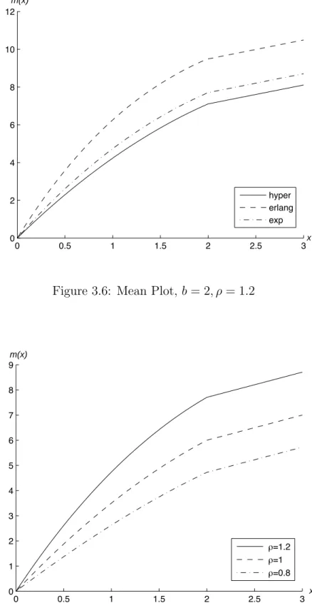
ρ= 0.8 Figure 3.4

Mean: m(x) ρ= 1 exp, erlang, hyper Figure 3.5

ρ= 1.2 Figure 3.6

Mean: m(x) ρ= 0.8,1,1.2 exp Figure 3.7

ρ= 0.8 Figure 3.8

Distribution: F(t, x= 1,2) ρ= 1 exp, erlang, hyper Figure 3.9

ρ= 1.2 Figure 3.10

Distribution: F(t, x= 1) ρ= 0.8,1,1.2 erlang Figure 3.11 Distribution: F(t, x= 1,2,3) ρ= 0.8 erlang Figure 3.12

ρ= 0.8 Figure 3.13

Density: f(t, x= 1,2) ρ= 1 exp, erlang, hyper Figure 3.14

ρ= 1.2 Figure 3.15

Density: f(t, x= 1) ρ= 0.8,1,1.2 erlang Figure 3.16 Density: f(t, x= 1,2,3) ρ= 0.8 erlang Figure 3.17

Note:

1. Figure 3.8,3.9,3.10 3.13, 3.14 and 3.15 include two sets of three curves for x=1 and x=2.

2. b= 2.

Table 3.1: Plots Summary

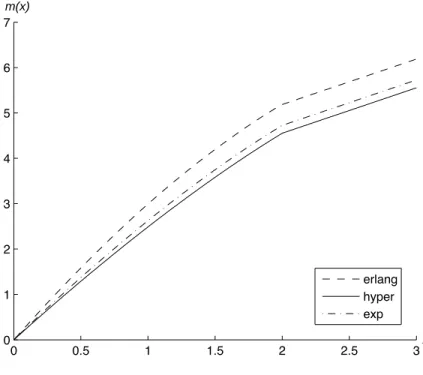
From Theorem 12, we have m(x) = (x−b) +m(b) when x > b. The linearity is illustrated in all mean plots. Also, from Theorem 13, we haveψ(s, x) = e−s(x−b)_{ψ(s, b)}

when x > b. This is reflected as a shift of the pdf curve as shown in Figure 3.17. Surprisingly, it is worth noting that as the variance of the service time becomes smaller, the meanm(x) becomes larger. Figure 3.4, 3.5 and 3.6 indicate thatmhyper(x)<

mexp(x) < merlang(x), x > 0. Moreover, in Figure 3.8,3.9 and 3.10, it is easy to see

that Bhyper <st. Bexp <st. Berlang.

Letm(x, b) be the mean first passage time parameterized by the balking threshold b. Figure 3.18 numerically verifies the following obvious identity:

by using the exponential service time and x∗ = 1, b = 3.

3.8

Concluding Remarks

In this chapter, we have developed an alternative method to study the first passage time problem for the M/P H/1 queues with wait-based balking via fluid models. The two models are connected by the construction illustrated in Section 3.5. We used elementary techniques to analyze the first passage time problem for the fluid model and obtained explicit solutions for the balking model. The method can also be applied to the dam model where service requirement is truncated if the complete admission of an arriving customer causes the workload to go beyond a given level.