5411.pdf



















DISEASE
MAPPING
OF
SYPHILIS
IN
FORSYTH
COUNTY,
NORTH


CAROLINA
WITH
ENHANCED
GEOPRIVACY
AND
SPATIAL


RESOLUTION














Lani
Clough














A
thesis
submitted
to
the
faculty
of
the
University
of
North
Carolina
at


Chapel
Hill
in
partial
fulfillment
of
the
requirements
for
the
degree


of
Masters
in
Science
in
the
Gillings
School
of
Global
Public
Health


(Environmental
Sciences
and
Engineering).











Chapel
Hill


2012





Approved
by:





Dr.
Marc
Serre





Dr.
Jacqueline
MacDonald

















ABSTRACT





LANI
CLOUGH:
Disease
mapping
of
syphilis
in
Forsyth
County,
North
Carolina
with
enhanced
 geoprivacy
and
spatial
resolution


(Under
the
direction
of
Dr.
Marc
Serre)
 



 This
paper
refines
the
spatial
resolution
of
disease
maps
by
making
use
of
geomasked


syphilis
cases
moved
by
a
random
displacement
to
preserve
their
anonymity.

Syphilis
cases
are


processed
using
the
Uniform
Model
Bayesian
Maximum
Entropy
(UMBME)
method
to
correct


for
the
small
number
problem.
Furthermore,
a
moving
window
approach
is
introduced
to
create


ubiquitous
areas
where
geomasked
cases
are
aggregated.
The
introduction
of
these
ubiquitous


areas
can
control
the
modifiable
areal
unit
problem
and
the
edge
effect
present
in
conventional


methods.

Our
hypothesis
is
this
approach
will
better
delineate
the
geographical
extent
of


clusters,
improving
outbreak
detection
and
reducing
the
ambiguous
and
spatially
incorrect


results
of
past
methodologies.
This
study
reveals
the
appearance
of
new
hotspots,
increased


connectivity
between
hotspots,
and
places
hot
spots
in
their
actual
locations.

This
specific


information
is
extremely
relevant
for
public
health
intervention
as
it
provides
the
ability
to


target
precise
locations.







iii








TABLE
OF
CONTENTS


LIST
OF
TABLES ...iv


LIST
OF
FIGURES ...v


Chapter


I.



INTRODUCTION ...1


II.



METHODS...5






Study
Population
and
Data
Preparation ... 5






Incidence
Areas... 7






Syphilis
Incidence
Rates ... 9






Spatial‐temporal
Analysis
and
Incidence
Mapping...11






Cross
Validation
of
BME
Methods...12


III.



RESULTS... 14


IV.



CONCLUSIONS... 19


REFERENCES... 20


















































LIST
OF
TABLES


Table



 1.
MSE
of
UG,
AG
methods
and
PCMSE
as
a
function
of
population
percentile

……….

16







































































v


LIST
OF
FIGURES


Figure


1. Arbitrary
and
ubiquitous
incidence
areas
in
Forsyth
County,
NC
………...8


2. Spatial
and
Temporal
Covariance
Models………...15


3. The
percent
change
in
MSE
from
AG
to
UG
as
a
function
of
the



population
percentile………..16
 


4. BME
maps
of
the
AG
&
UG
methods
in
February‐July,
2009
(the



peak
of
the
outbreak)………..17

 


5. UG
method
time
series
of
the
Forysth
County
Outbreak
(2009‐2010)………19



































1.
INTRODUCTION


The
southeastern
region
of
the
United
States
has
consistently
experienced
higher
rates


of
syphilis
than
other
areas
in
the
US
(Sena,
2007,
Rosenberg
1998).
The
southeast’s
persistent


syphilis
 prevalence
 is
 likely
 a
 result
 of:
 the
 racial/ethnic
 distribution
 of
 residents;
 the


population’s
 sexual
 mixing
 patterns;
 drug
 use;
 the
 exchange
 of
 drugs
 and
 money
 for
 sex;


poverty;
 and
 reduced
 access
 and
 poor
 usage
 of
 health
 care
 (Doherty,
 2011;
 NC,
 2010;


Rosenberg,
 1998;
 Sena,
 2007).
 In
 1999,
 the
 Centers
 for
 Disease
 Control
 (CDC)
 created
 the


Syphilis
 Elimination
 program
 (SEP)
 for
 the
 southeast
 region.
 
 In
 North
 Carolina
 extensive


funding
was
focused
on
the
counties
with
the
highest
incidence
of
syphilis
(Mecklenburg,
Wake,


Durham,
Guilford,
Forsyth,
and
Robeson)
and
syphilis
incidence
statewide
was
greatly
reduced.


In
2004,
resources
provided
for
SEP
began
to
decline
and
syphilis
rates
increased
(NC,
2010).




In
2009,
North
Carolina
experienced
an
84%
(937
cases)
increase
in
infectious
syphilis


cases
 from
 2008
 (509
 cases).
 
 This
 resurgence
 occurred
 throughout
 the
 state,
 especially
 in


counties
the
interstate
highways
85
and
40
pass
through.

The
increase
was
clearly
evident
in


Forsyth
County
which
encountered
more
than
a
fourfold
rise
in
infectious
syphilis
cases
from


46
in
2008
to
195
in
2009
(NC,
2010).

In
2010,
the
Forsyth
syphilis
epidemic
began
to
wane


and
only
103
cases
were
reported
(NC,
2011).

The
incidence
significantly
decreased
again
in


2011
to
47
cases
returning
to
the
county’s
endemic
levels
(NC,
2012).
In
North
Carolina,
syphilis


outbreaks
 in
 the
 past
 20
 years
 have
 been
 concentrated
 in
 counties
 with
 elevated
 syphilis


incidence
 where
 rates
 during
 outbreaks
 increase
 to
 levels
 seldom
 found
 in
 the
 United
 States


(Doherty,
2011).




Beyond
 the
 concern
 for
 syphilis
 morbidity,
 ulcerative
 sexually
 transmitted
 infections





2


HIV
 positive
 (NC,
 2010;
 Sena,
 2008).
 In
 the
 outbreak
 in
 Forsyth
 County,
 the
 syphilis
 cases


increased
significantly
within
the
HIV
positive
community.
There
are
considerable
concerns
a


syphilis
outbreak
will
lead
to
increased
HIV
morbidity
in
North
Carolina
(NC,
2010).



Understanding,
 targeting
and
controlling
syphilis
outbreaks
is
an
evident
and
genuine


concern
 for
 the
 state
 of
 North
 Carolina
 (NC,
 2010).
 
 
 Spatiotemporal
 analysis
 of
 sexually


transmitted
 infections
 has
 been
 effective
 in
 defining
 core
 areas
 of
 infection,
 providing
 insight


into
patterns
of
transmission
and
assisting
health
policy
makers
in
increasing
the
effectiveness


and
reducing
the
costs
of
interventions
(Choi,
2003;
Gesink,
2006;
Hampton,
2011;
Hanafi‐Bojd,


2012;
Law,
2004;
Zenilman,
1998).



The
 Bayesian
 Maximum
 Entropy
 (BME)
 approach
 of
 contemporary
 geostatistics
 is
 a


spatiotemporal
 analysis
 structure.
 BME
 analyses
 have
 long
 been
 successfully
 used
 in
 a
 wide


range
 of
 applications
 for
 both
 public
 health
 and
 environmental
 concerns
 and
 the
 theory
 is


highly
developed
(Allhouse,
2009;
Choi,
2003;
De
Nazelle,
2010;
Gesink,
2006;
Hampton,
2011;


Law,
2006;
Orton,
2008;
Serre,
2004).




Modern
non‐linear
geostatistics,
such
as
BME
can
incorporate
both
known
data
(hard)


and
 data
 modeled
 by
 various
 distributions,
 such
 as
 uniform
 (soft).
 
 In
 the
 field
 of
 linear


geostatistics,
 methods
 such
 as
 kriging
 are
 used
 to
 predict
 unknown
 values
 (k)
 given
 a
 prior


knowledge
base
of
known
observations
(h).

The
unknown
random
variable
is
assumed
to
be


normally
 distributed,
 with
 a
 mean
 of
mk|h,
 and
 a
 variance
Ck|h,
 where
C
 is
 the
 covariance
 of
k


given
h.

mk|h
is
the
kriging
mean
and
referred
to
as
the
best
linear
unbiased
estimator
(BLUE)
in


geostatistics
 and
 the
 best
 linear
 unbiased
 predictor
 (BLUP)
 in
 statistics.
 
 The
 kriging
 mean
 is


linear,
unbiased
and
the
best
estimator
that
minimizes
the
estimation
error
variance.




In
 public
 health
 analyses,
 BME
 techniques
 that
 can
 incorporate
 soft
 data
 have


fundamental
benefits
over
other
methods.
Disease
incidence
measures
express
varying
levels
of


space
and
time.

This
is
especially
relevant
for
STD
outbreaks
which
can
fluctuate
greatly
within


geographic
areas
and
temporal
periods.
The
BME
techniques
provide
predictions
that
minimize


the
mean
squared
error
of
space/time
random
fields
(S/TRFs)
to
accurately
model
rates
(Choi,


2003).



Geospatial
 analysis
 of
 incidence
 rates
 can
 be
 challenging.
 
 Universally,
 incidence
 rates


are
 created
 by
 aggregating
 individual‐level
 data
 to
 pre‐existing
 administrative
 areas,
 such
 as


counties
 or
 census
 block
 groups
 (CBGs)
 and
 assigning
 the
 data
 to
 the
 centroid
in
an
effort
to


protect
 patient
 privacy.
 
 Protecting
 patient
 privacy
 with
 this
 method
 generally
 destroys


pertinent
information
needed
to
address
important
public
health
concerns
(Kamel,
2006)
and


produces
spatial
uncertainty
also
known
as
the
Modifiable
Areal
Unit
Problem
(MAUP)
(Bailey


and
Gatrell
1995;
Kamel,
2006;
Ratcliffe,
1999).

The
MAUP
is
composed
of
two
problems‐
1)


the
 size
 of
 each
 of
 the
 aggregation
 zones
 and
2)
 the
 shapes
 of
 the
 areal
 units.
 
 The
 size
issue


concerns
the
large
differences
in
rates
that
can
be
obtained
when
aggregation
areas
are
reduced


or
enlarged,
such
as
enlarging
census
block
group
rates
to
county
or
state
rates.

Furthermore,


the
 shape
 problem
 refers
 to
 the
 variance
 of
 sizes
 and
 shapes
 within
 a
 set
 areal
 zones.
 
 For


example,
 the
 areas
 of
 California
 and
 Alaska
 are
 tremendously
 larger
 than
 the
 areas
 of
 Rhode


Island
 or
 Maryland,
 although
 they
 are
 each
 categorized
 as
 the
 same
 aggregation
 unit,
 a
 state.



This
variation
creates
considerable
differences
in
rates
for
each
state.




The
 capacity
 of
 an
 investigator
 to
 identify
 disease
 clusters
 or
 the
 progression
 of
 an


outbreak
is
increasingly
limited
when
the
data
is
aggregated
to
large
areas,
such
as
counties
or


states.
 Displacing
 rates
 to
 the
 centroids
 of
 these
 administrative
 boundaries
 can
 produce


misleading
results
that
are
exaggerated
when
a
hot
spot
is
located
on
the
boundary
of
two
or


more
aggregation
areas.

An
example
of
this
effect
is
the
displacement
of
a
hot
spot
from
its
true


location
on
a
boundary
to
an
artificial
location
at
the
centroid
or
the
complete
loss
of
a
hot
spot.






4


The
edge
effect
can
be
lessened
by
reducing
the
aggregation
level.

However
reducing


the
scale
of
the
data
also
introduces
uncertainty
or
noise
resulting
from
unreliable
rates,
known


as
the
“small
number
problem”.
The
small
number
problem
can
obscure
spatial
patterns
and
if


not
 corrected
 result
 in
 an
 inappropriate
 interpretation
 of
 the
 health
 outcome.
 When


researching
rare
diseases
such
as
syphilis,
computing
crude
rates
from
data
with
high
spatial


resolution
 creates
 statistical
 concerns
 due
 to
 the
 scarcity
 of
 the
 data
 set.
 
 The
 variation
 in


populations
 within
 the
 aggregation
 areas
 will
 lead
 to
 a
 field
 of
 disease
 counts
 dominated
 by


locations
 with
 relatively
 low
 populations
 because
 their
 incidence
 rates
 will
 be
 artificially


elevated
(Choi,
2003;
Hampton,
2011;
Goovaerts,
2005a;
Goovaerts,
2005b).



Extensive
 work
 has
 been
 performed
 to
 remove
 the
 small
 number
 problem
 while


preserving
 spatial
 resolution.
 
 Multiple
 smoothing
 algorithms
 have
 been
 developed
 to
 more


accurately
 assess
 true
 incidence
 rates
 (also
 known
 as
 latent
 rates)
 and
 penalize
 areas
 with


small
populations
to
create
a
more
even
rate
field.
These
methods
introduce
a
variance
measure


which
is
a
function
of
the
population
providing
a
measure
of
uncertainty
for
each
location
and


penalizing
 aggregation
 areas
 with
 small
 populations
 
 (Hampton,
 2011;
 Goovaerts,
 2005a;


Goovaerts,
2005b).



Two
 advanced
 smoothing
 methods
 are
 Poisson
 Kriging
 (PK)
 and
 Uniform
 Model


Bayesian
Maximum
Entropy
(UMBME).
Poisson
Kriging
exhibits
a
strong
smoothing
effect
and


has
 been
 shown
 to
 be
 more
 accurate
 in
 estimating
 latent
 disease
 rates
 than
 unsmoothed


methods.

UMBME,
however
has
been
found
to
produce
more
accurate
rate
estimates
than
PK
in


a
 study
 of
 HIV
 in
 North
 Carolina
 while
 reducing
 over‐smoothing
 and
 retaining
 the
 ability
 to


effectively
detect
hotspots
(Hampton,
2011).


Additional
 increases
 in
 spatial
 resolution
 can
 be
 acquired
 while
 maintaining
 patient


privacy
by
employing
the
Donut
Method
of
geomasking.

This
method
randomly
relocates
each


of
patient
privacy
while
maintaining
the
spatial
resolution
necessary
for
cluster
and
outbreak


detection.
It
is
especially
effective
in
locations
with
high
threats
to
geoprivacy
(Allhouse,
2010;


Hampton,
 2010).
 
 Unfortunately
 no
 studies
 have
 been
 conducted
 which
 take
 advantage
 of


geomasked
 data
 sets.
 
 Currently
 maps
 created
 without
 geomasked
 data
 exhibit:
 1)
 islands
 of


higher
and
lower
incidence
at
the
centroids;
2)
the
edge
effect;
3)
masking
of
hotspots;
and
4)
a


background
rate
greater
than
zero.



Using
 state
 health
 department
 data,
 the
 goal
 of
 this
 paper
 is
 the
 Bayesian
 Maximum


Entropy
space/time
analysis
of
the
infectious
syphilis
incidence
among
the
population
tested
in


Forsyth
County
from
1999‐2011.
This
paper
advances
the
methodology
for
outbreak
analysis


by
 refining
 spatial
 resolution
 with
 the
 use
 of
 geomasked
 data.
 
 The
 small
 number
 problem
 is


also
removed
by
employing
Uniform
Model
Bayesian
Maximum
Entropy.
Additionally,
a
global


moving
window
approach
is
utilized
to
control
the
MAUP
and
the
edge
effect.

Our
hypothesis
is


this
 method
 will
 better
 delineate
 the
 geographic
 extent
 of
 clusters,
 reducing
 some
 of
 the








2.
METHODS


Study
Population
and
Data
Preparation



 The
 study
 population
 for
 this
 work
 includes
 all
 Forsyth
 County
 residents
 in
 the
 time


period
 of
 1999‐2011.
 
 A
 syphilis
 case
 is
 defined
 as
 a
 Forsyth
 County
 resident
 infected
 with


syphilis,
and
diagnosed
between
January
1,
1999
and
April
30,
2011.

The
data
for
the
study
was


acquired
from
the
North
Carolina
Department
of
Public
Health’s
Communicable
Disease
Branch.



North
Carolina
Health
Care
providers
and
laboratories
are
required
to
complete
communicable


disease
 report
 cards
 for
 each
 diagnosed
 case
 of
 syphilis
 and
 submit
 these
 reports
 to
 the


appropriate
county
health
department.

These
report
cards
include
information
on
the
patient’s


disease,
 report
 date,
 date
 of
 disease
 onset,
 residence
 at
 diagnosis,
 syphilis
 disease
 stage
 and


limited
 demographic
 information.
 Both
 the
 University
 of
 North
 Carolina
 institutional
 review


board
 and
 the
 CDC
 internal
 review
 board
 have
 approved
 the
 use
 of
 this
 data
 for
 space‐time


analysis.



Self‐reported
 case
 residential
 addresses
 were
 reformated
 and
 corrected
 with
 Satori


Bulk
Mailer
software
(Satori
Software
Inc.,
Seattle,
WA)
before
geocoding
to
optimize
the
match


rate
 of
 addresses.
 Patient
 residences
 were
 then
 geocoded
 using
 ESRI’s
 ArcGIS
 9.3.1
 (ESRI,


Redlands,
 California)
 and
 matched
 to
 three
 geographic
 locators
 used
 by
 the
 State
 of
 North


Carolina.
The
primary
locator
was
created
by
the
North
Carolina
Department
of
Transportation


and
 contains
 street‐level
 geographic
 data.
 The
 secondary
 locator
 was
 created
 by
 the
 North


Carolina
 Emergency
 Response
 System
 and
 contains
 point
 locations
 for
 North
 Carolina


households.
 
 The
 tertiary
 locator
 was
 created
 using
 ESRI’s
 2006
 Street
 Map
 shapefile
 (ESRI,


and
 military
 bases.
 Cases
 with
 a
 post
 office
 box
 address
 were
 spatially
 assigned
 to
 that
 post


office
address.

Demographic
information
was
removed
prior
to
the
geocoding
of
the
data.





Approximately
83%
of
the
records
in
the
time
period
were
successfully
geocoded
to
a


location
(497).

Cases
which
were
not
geocoded
(104)
are
excluded
from
the
analysis.

Of
the


cases
not
geocoded,
36
were
in
2009
and
16
in
2010.

The
primary
reasons
why
these
addresses


did
not
geocode
are:
1)
no
address
was
provided;
2)
non‐existent
addresses
were
provided;
3)


the
 locators
 are
 missing
 street
 segments;
 4)
 incorrect
 addresses
 (misspellings,
 abbreviated


street
 names
 and
 improper
 use
 of
 rural
 routes).
 
 After
 geocoding,
 the
 data
 were
 geomasked


using
the
Donut
Method
(Allshouse,
2010;
Hampton,
2010).



The
focus
of
this
study
is
incidence
rates
thus
the
syphilis
diagnosis
stage
was
used
to


estimate
the
date
the
patient
acquired
the
disease.

Five
stage
codes
are
included
in
the
dataset


and
represent
the
following:
Stage
1
is
a
primary
syphilis
infection,
Stage
2
is
secondary
syphilis


infection
and
the
third
stage
is
early
latent
syphilis.

Cases
with
primary,
secondary
and
early


latent
syphilis
are
generally
categorized
as
‘early
syphilis’
and
are
the
stages
when
the
disease


can
be
transmitted
to
sexual
partners.

The
fourth
and
fifth
stages
are
considered
latent
syphilis


and
 not
 infectious
 thus
 are
 excluded
 from
 the
 analysis
 (Doherty,
 2002;
 NC,
 2010).
 
 We


estimated
the
date
of
infection
using
the
provided
diagnosis
date
and
median
latency
period
for


each
 syphilis
 disease
 stage.
 Primary
 syphilis
 cases
 were
 back
 estimated
 45
 days,
 secondary


syphilis
 was
 back
 estimated
 90
 days,
 and
 early
 latent
 syphilis
 was
 back
 estimated
 183
 days


(Schumacher,
2005).






Incidence
Areas



 The
 incidence
 area
 is
 the
 geographic
 foundation
 on
 which
 a
 rate
 is
 defined.
 
 It
 can
 be


thought
of
as
a
set
of
cases
in
a
defined
area.
An
incidence
area
may
be
a
circular
or
complex





8


incidence
 area,
 a
 rate
 can
 be
 calculated
 and
 is
 assigned
 to
 an
 area’s
 centroid.
 
 Virtually
 all


incidence
 rates
 are
 calculated
 using
 administrative
 boundaries
 as
 their
 incidence
 areas.
 
 The


centroids
of
these
incidence
areas
are
often
arbitrarily
located
in
space
with
varying
distances


between
the
centroids.

This
creates
an
uneven
clustering
of
centroids
and
is
illustrated
in
the


arbitrary
 groups
 (AG)
 shown
 in
 Figure
 1.
 In
 this
 case,
 the
 AGs
 are
 census
 block
 groups
 in


Forsyth
County.
The
boundaries
of
the
census
block
groups,
now
referred
to
as
AGs
are
shown


as
thin
black
lines
and
their
centroids
are
black
triangles.
The
distribution
of
AG
centroids
and


the
large
variations
in
the
AG
sizes
and
shapes
in
Figure
1
clearly
shows
a
MAUP
and
a
strong


edge
effect.

……….




Figure
1:
Arbitrary
and
ubiquitous
incidence
areas
in
Forsyth
County,
NC







 The
MAUP
and
edge
effect
created
when
aggregating
to
arbitrary
incidence
groups
can


be
corrected
by
enriching
an
AG
dataset
with
incidence
area
centroids
based
on
a
regular
grid


(shown
as
turquoise
circles
in
Figure
1).

A
moveable
sub‐region
of
overlapping
perfect
circles


without
 the
 variability
 caused
 by
 size
 and
 shape
 creating
 a
 framework
 for
 the
 analysis
 and


removing
 the
 MAUP
 (Bailey,
 1995).
 
 Furthermore,
 overlapping
 the
 boundaries
 of
 the
 circles


reduces
the
edge
effect.




 The
 size
 of
 the
 circles/incidence
 areas
 and
 density
 of
 the
 grid
 can
 be
 increased
 or


decreased
according
to
project
needs.

Cases
located
within
each
of
these
grid‐based
incidence


areas,
which
we
will
refer
to
as
ubiquitous
groups
(UG)
are
identified
and
utilized
to
calculate
a


rate.

A
rate
is
then
assigned
to
each
centroid
(grid
point)
of
the
incidence
areas.

In
this
study,


two
data
sets
of
syphilis
incidence
were
created
and
compared,
AG
and
UG.







Syphilis
Incidence
Rates



 To
 create
 the
 AG
 dataset,
 the
 populations
 and
 boundaries
 of
 census
 block
 groups
 in


2000
packaged
in
a
US
Census
census
block
group
shapefile
(US
Census,
2009)
were
used.

The


AG
 geographic
 centroids
 were
 calculated
 using
 this
 shapefile
 in
 ESRI’s
 ArcGIS
 10
 (ESRI,


Redlands,
CA).

AG
cases
were
aggregated
spatially
by
AG
boundaries
(in
this
case
census
block


groups),
 and
 temporally
 with
 a
 rolling
 time
 period
 of
 6
 months
 to
 lessen
 the
 small
 number


problem.

The
crude
incidence
rate
at
location
si
and
incidence
period
of
duration
T expressed
in


years
(i.e.
T =
0.5yr
for
a
6
month
incidence),
centered
at
time
tj
is
denoted
as
Rij
and
calculated


as
Rij=yij/(nijT). Where yij
is
the
number
of
syphilis
cases
within
the
incidence
area
i,
nij
is
the


population
 at
 time
tj.
 
 The
 population
 growth
 was
 also
 incorporated
 into
 the
 crude
 rate


calculation
 through
 a
 linear
 interpolation
 of
 the
 census
 block
 group
 population
 for
 all
 12‐64‐

year‐olds
in
2000
and
2007
assuming
positive
growth
over
the
time
period.
Time
periods
that


did
not
contain
syphilis
records
were
assumed
to
have
a
rate
of
0.



 The
UG
dataset
consists
of
the
AG
data
combined
with
grid‐based
ubiquitous
incidence





10


€

D=1

n Aa

π

∑

    

 * f ,
where
D
is
the
distance
between
UG
centroids
in
the
grid,
Aa
is
the
area


of
 each
 AG
 and
f
 is
 the
 factor
 to
 increase
 or
 reduce
 the
 grid.
 For
 this
 study,
f
 =
 .65
 and
D =


0.5miles
to
create
a
fine
grid
lattice
throughout
the
study
area
and
comprehensively
reduce
the


MAUP.

Grid
points
outside
of
Forsyth
County
were
discarded.
Each
grid
point
was
used
as
the


centroid
of
a
UG.





 The
UG’s
associated
area
of
influence
is
a
perfect
circle
and
it’s
area
is
calculated
by
π

€

ri 2_,

where


€

ri
 is
 the
 optimized
 radius
 length.
 


€

ri
 is
 calculated
 from
 the
 inverse
 weighted
 distance


average
 of
 the
 radius
 of
 the
 five
 closest
 AGs
 where
 distance
 is
 penalized
 in
 the
 following


formula:


€

r

_i

=

w

_j

*

r

_j

j=1 5

∑

,
where


€

w

_j

=

d

_ij−1

*

d

_ij−1

j=1 5

∑

,


and
w
is
the
weight
given
to
each
area
value


in
the
mean
calculation,
d
is
the
distance
of
the
AG
centroid
to
the
UG
centroid,
i
is
the
spatial


location
and
j
is
the
identifier
for
each
AG
centroid.

The
changing
size
of
the
UGs
in
relation
to


their
local
AGs
can
also
be
seen
in
Figure
1.





 Next,
the
population
for
each
UG,
 
was
calculated
from
as
a
function
of
the
area
of
the


AGs
lying
within
the
UG:


€

ni=

Aa∩ i

Aa

∑

*PAa,
where
Aa
is
the
area
of
the
AGs
and
PAa
is
the


population
of
Aa
at
the
time
period.

The
population
was
assumed
to
be
uniformly
distributed


within
the
AG.





 The
number
of
cases
within
each
UG
was
calculated
as
a
function
of
the
probability
each


case
 is
 within
 a
 UG
 at
 a
 selected
 time
 period.
 The
 following
 is
 known
 about
 the
 geomasked


points:
1)
each
point
is
geomasked
within
the
AG
they
are
located
in
and
2)
the
maximum
and


minimum
distance
a
case
can
be
moved
from
its
original
location,
creating
a
donut
around
each


case
 (this
 information
 can
 only
 be
 accessed
 at
 the
 NC
 Public
 Health
 Department
 by
 selected


calculated
 as:


€

R

_i

≈

w

_li l=1

N

∑

n

_i

*

T

.
 Where


€

w_li
 is
 the
 probability
 case
 
 is
 in
 area
 ,
N
 is
 the
 total


number
of
cases
in
 
and


€

w

_li

=

AR

l

∩

UG

i

AR

_l .

Furthermore,


€

AR

_l

=

DR

_l

∩

AG

_lwhere


€

DR

_l
is


the
 size
 of
 the
 geomask
 donut
 before
 the
 restriction
 the
 area
 of
 the
 donut
 outside
 of
 the
 AG


must
be
removed,


€

AGis
the
area
of
the
AG.



€

AR

_l
is
the
area
the
geomasked
point
was
located


at
geocoding
and
prior
to
geomasking.



 Finally,
 to
 comprehensively
 remove
 the
 small
 number
 problem,
 UMBME
 rates
 were


calculated
for
both
the
AG
and
UG
data
sets.

The
Uniform
Model
BME
method
can
be
described


as
 follows.
 
 A
 soft
 datum
 for
 the
 true
 incidence
 rate,
Xij,
 can
 be
 described
 by
 a
 uniform


probability
 distribution
 and
 constructed
 where
 α
 >
 0.5
 and

€

R

_ij

−

α

n

_ij

*

T

<

X

ij

<=

R

ij

+

α

n

_ij

*

T

.



Data
that
have
been
smoothed
by
UMBME
should
be
considered
and
treated
as
soft
data
in
the


mapping
process
(Hampton,
2011).







Spatial­temporal
Analysis
and
Incidence
Mapping




 This
 work
 uses
 a
 BME
 geostatistical
 analysis
 to
 estimate
 the
 syphilis
 incidence
 in


Forsyth
County,
NC.

BME
utilizes
random
field
theory
to
create
incidence
estimates
where
the


mean
square
error
is
minimized
at
nodes
on
an
estimation
grid.

The
BME
framework
allows
for


the
incorporation
of
soft
data
modeled
by
a
distribution,
such
as
the
UMBME
data.
The
analysis


is
 performed
 over
 a
 space/time
 random
 field
 (S/TRF),
 which
 estimates
 the
 distribution
 of


incidence
rates
over
space
and
time
as
a
function
of
possible
field
moments.





 The
BME
analysis
can
be
broken
into
three
main
steps.

The
first
step
is
to
examine
the


data
 to
 obtain
 a
 prior
 probability
 density
 function
 (PDF)
 of
 the
 S/TRF
 for
 syphilis
 incidence.





12


Third,
the
posterior
PDF
is
used
to
isolate
the
incidence
to
derive
space‐time
maps
of
Forsyth


County
incidence
represented
as
spatial
random
fields.




 The
inputs
for
the
spatial
temporal
model
are:
the
mean
trend
for
the
data,
a
covariance


model,
and
the
calculation
parameters:
1)
the
UBME
rates
(soft
data);
2)
the
maximum
number


of
data
points
that
can
contribute
to
an
estimate;
3)
the
estimate’s
spatial
search
radius
4)
and


the
 coordinate
 of
 the
 estimate
 point.
 
 The
 output
 for
 the
 BME
 analysis
 is
 the
 moments
 of
 the


BME
 posterior
 PDF,
 specifically
 the
 expected
 value
 for
 the
 estimate
 point
 and
 the
 variance
 of


the
moment
(Akita,
2007;
Allhouse,
2009;
De
Nazelle,
2011;
Hampton,
2011;
Law,
2004;
Serre,


2004).

The
numerical
processing
of
this
data
was
performed
using
MATLAB
7.8
(Mathworks,


Natick,
MA)
and
the
BMElib
package
(BMElab,
UNC‐CH).





 The
 mean
 trend
 is
 considered
 to
 be
 a
 deterministic
 function
 and
 the
 residual
 S/TRF


models
the
uncertainties
and
variability
associated
with
the
dataset
over
space
and
time
(Serre,


2004).
Prior
to
the
BME
analysis,
the
mean
trend
was
removed
from
the
dataset,
smoothing
the


spatiotemporal
 fluctuations
 and
 resulting
 in
 a
 residual
 field
 that
 is
 homogenous
 in
 space
 and


stationary
in
time.






 Covariance
 is
 a
 measure
 of
 association
 between
 two
 variables,
 whereas
 a
 covariance


function
describes
the
variance
and
characterizes
the
consistent
tendencies
and
dependencies


of
 a
 random
 field
 or
 variable,
 such
 as
 a
 space/time
 random
 field
 (Serre,
 2004).
 
 S/TRF


covariance
 functions
 provide
 a
 quantitative
 description
 of
 the
 correlation
 between
 pairs
 of


observations
 as
 a
 function
 of
 the
 inter‐pair
 distances.
 The
 overall
 disease
 patterns
 are


illustrated
by
the
nature
of
the
model
as
the
distance
from
the
sill
increases.

The
general
spatial


variability
is
shown
in
the
sill
(the
covariance
at
distance
0)
and
by
the
slope
of
the
model
near


the
origin.
The
larger
the
sill
and
the
steeper
the
slope,
the
greater
the
spatial
variability.

The


or
loses
95%
of
the
inter‐pair
correlation)
identifies
the
area
in
which
neighboring
observations


influence
the
rate
at
a
location
(De
Nazelle,
2010;
Law,
2004).






Cross­Validation
of
BME
Methods




 A
cross‐validation
of
the
AG
and
UG
methods
was
conducted
and
compared
to
identify


the
most
accurate
method
to
model
the
syphilis
rates.

In
the
cross
validation,
an
observed
value


was
 removed
 from
 the
 dataset
 and
 the
 BME
 method
 was
 used
 to
 calculate
 the
 rate
 at
 that


location.

The
observation
is
then
returned
to
the
data
set
and
the
next
value
is
removed
and
its


estimate
is
calculated.

This
process
is
repeated
for
each
of
the
data
points.

The
error
for
each


data
point
is
then
calculated.
The
cross‐validation
errors
for
each
method
are
then
summarized


as
 a
 function
 of
 the
 mean
 square
 errors
 (MSE).
 The
 MSE
 quantifies
 the
 amount
 an
 estimator


varies
from
a
known
rate
and
can
assess
the
performance
of
an
estimator
through
its
variation


and
 unbiasedness.
 
 An
 MSE
 of
 zero
 demonstrates
 the
 estimator
 perfectly
 predicts
 an


observation,
 and
 the
 MSE
 is
 always
 a
 positive
 value.
 
 The
 MSE
 is
 effective
 for
 comparing
 the


ability
 of
 varying
 estimators
 to
 predict
 known
 observations,
 where
 the
 estimator
 with
 the


smallest
MSE
is
considered
the
best
predictor
for
the
data
set.
To
compare
the
MSE
between
the


methods,
only
the
AG
data
points
contained
within
the
UG
and
AG
datasets
are
evaluated
in
the


MSE
estimate
(28,290
points).

The
MSE
formula
is:




€

MSE

_AG

=

1

n

A

ˆ

G

_ij

−

AG

_ij

(

)

2

∑

MSE

_UG

=

1

n

U

ˆ

G

_AGij

⊂

U

G

ˆ

_ij

(

)

−

AG

_ij

(

)

2

∑




where
 
is
the
value
estimated
in
the
cross
validation,
i
is
the
spatial
location,
and
j
is
the


temporal
period.

AG
is
the
calculated
rate,
 
are
the
cross
validation
estimated
values
for
UG





14


€

UG

AGij

⊂

UG

ij

=

AG

ij

∩

UG

ij.

To
compare
the
MSE
between
the
methods,
the
percent
change


in
the
mean
square
error
(PCMSE)
is
calculated
by:



€

PCMSE_UG =100 * MSEUG−MSEAG

MSE_AG      .
A
negative
PCMSE
demonstrates
the
percent
improvement
 in
the
estimation
accuracy
from
the
first
method
to
the
second
(De
Nazelle,
2011).
 
 The
latent
rate
is
the
most
appropriate
measure
to
compare
the
ability
of
a
method
to


predict
 a
 rate.
 
 The
 latent
 incidence
 rate
 of
 disease
 in
 a
 given
 region i can
 be
 defined
 as:

€

X

_i

=

ni→∞

lim

r

j

n

_iwhereXi is
the
latent
disease
rate,
Yi is the number of new cases of disease, andniis


the
size
of
the
population
at
risk
in
areai. This
states
as
the
population
approaches
infinity,
the


observed
rate
reaches
the
latent
rate.

In
practice,
the
latent
rate
can
be
estimated
by
stratifying


the
 MSE
 results
 by
 the
 population
 percentile
 (Hampton,
 2011).
 
 A
 method
 is
 effective
 if
 the














3.
RESULTS






 The
analysis
of
the
mean
trend
resulted
in
the
following
equation:
mZ(s,t) = ms(s) + mt(t)


,
where:
ms(s)
is
the
spatial
component
of
the
mean
trend
and
mt(t)
is
the
temporal
component


of
 the
 mean
 trend
 using
 an
 exponential
 kernal
 smoothing
 to
 obtain
 geographic
 and
 temporal


averages.
 
 For
 this
 model,
ms(s) is
 40km
 with
 a
 1km
 smoothing
 range
 and
mt(t)
 is
 15
 months


with
a
6
month
smoothing
range.





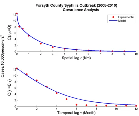
 Next
 the
 experimental
 covariances
 of
 the
 residual
 space‐time
 incidence
 field
 and
 a


covariance
model
of
these
experimental
values
were
calculated
and
are
shown
in
Figure
2.

For


this
 data
 set
 the
 covariance
 model
 is
 a
 non‐separable
 model
 with
 the
 superposition
 of
 three


exponential
 and
 gaussian
 models
 with
 varying
 spatial
 and
 temporal
 scales,
 as
 shown
 in
 the


following
 equation:
 ………


Cx(r,t) = c1 exp(-3r/ar1)(-3t/at1) + c2 exp(-3r/ar2)(3t22/at22) + c3 exp (-3r/ar3)(-3t/at3),
 where
c1=


3cases/10,000person‐yrs2_,
ar

1=
0.2km,
at1=
8months,
c2=
.5cases/10,000person‐yrs2,
ar2=
4km,



at2=24months
 and
c3=
 8.9cases/10,000person‐yrs2,
ar3=
 5.5km,
 
at3 =
 11
 months.
 
 The
 spatial


covariance
model
indicates
high
variability
within
the
observations
and
an
autocorrelation
with


a
relatively
short
range‐
4km
(less
than
10%
of
the
study
area)
that
sharply
drops.
Temporally,


there
 is
 significantly
 less
 variability
 and
 the
 drop
 in
 autocorrelation
 is
 slow
 and
 smooth
 over


long
time
periods‐
2
years,
the
duration
of
the
Forsyth
outbreak.







16





Figure
2:
Spatial
and
Temporal
Covariance
Models






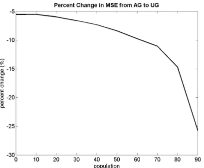
 Next,
 a
 cross‐validation
 analysis
 was
 performed
 on
 the
 two
 methods,
 AG
 and
 UG
 to


define
 the
 method
 which
 most
 accurately
 models
 the
 latent
 rate.
 
 The
 cross‐validation


demonstrated
the
UG
model
performed
noticeably
better
in
predicting
the
latent
rate
than
the


AG
model.
This
is
revealed
in
the
PCMSE
which
decreases
as
the
population
percentile
increases


as
shown
in
Figure
3.






Figure
3:
The
percent
change
in
MSE
from
AG
to
UG
as
a
function
of
the
population
percentile






 The
 corresponding
 MSE
 values
 for
 the
 AG
 and
 UG
 methods
 are
 shown
 along
 with
 the


population
 percentile
 and
 the
 PCMSE
 in
 Table
 1.
 These
 results
 further
 confirm
 the
 UG
 rates


minimize
the
MSE
and
more
accurately
model
the
latent
syphilis
incidence
rates.






Table
1:
MSE
of
UG,
AG
methods
and
PCMSE
as
a
function
of
population
percentile

 Population


Percentile


MSE
AG
 UMBME


MSE
UG
 UMBME


Percent
change
 AG
to
UG


0
 4.06E‐07
 3.83E‐07
 ‐5.5


10
 3.67E‐07
 3.47E‐07
 ‐5.5


20
 3.09E‐07
 2.90E‐07
 ‐5.9


30
 2.97E‐07
 2.78E‐07
 ‐6.6


40
 2.83E‐07
 2.62E‐07
 ‐7.3


50
 2.50E‐07
 2.29E‐07
 ‐8.4


60
 2.12E‐07
 1.91E‐07
 ‐9.8


70
 1.88E‐07
 1.67E‐07
 ‐11.1


80
 8.34E‐08
 7.11E‐08
 ‐14.7


90
 5.54E‐08
 4.11E‐08
 ‐25.8






 Furthermore
the
differences
in
the
methods
are
illustrated
visually
in
the
maps
of
the


two
approaches
as
shown
in
Figure
4.

Two
black
boxes
are
displayed
in
the
figure.

The
first


box
 in
 the
 center
 of
 the
 map,
 shows
 the
 increased
 connectivity
 within
 the
 UG
 method.
 
 The





18


locations.
In
the
AG
map,
the
lower
black
box
shows
a
hot
spot
placed
at
the
centroid
of
the
UG


and
 outside
 of
 the
 Winston‐Salem
 city
 limits.
 In
 contrast
 the
 UG
 method
 places
 the
 hotspot


within
the
Winston‐Salem
city
limits
and
between
a
park
and
mall.




 Overall,
 new
 hot
 spots
 appear
 in
 the
 UG
 map
 particularly
 in
 areas
 between
 spatial


aggregations.

This
demonstrates
the
AG
map
is
suffering
from
the
edge
effect.

Additionally,
the


spatial
resolution
is
improved
with
the
use
of
the
UG
method,
showing
new
hotspots,
increased


connectivity
between
hot
spots
and
placing
hot
spots
in
their
actual
locations.

Moreover,
the


background
 rate
 in
 the
 AG
 map
 is
 approximately
 five
 cases/10,000person‐years
 and
 the
 UG


method
corrects
this
flaw
by
resetting
the
background
rate
to
0.





 














Figure
4:
BME
maps
of
the
AG
&
UG
methods
in
February­July,
2009
(the
peak
of
the
 outbreak)




 



 The
BME
map
time
series
of
the
outbreak
for
selected
time
periods
is
shown
in
Figure
5.



A
movie
of
the
outbreak
can
be
found
at:
http://www.unc.edu/depts/case/BMElab/.

Endemic


levels
 of
 syphilis
 are
 found
 in
 hot
 spots
 with
 an
 incidence
 of
 approximately


Lewisville
 and
 Kernersville.
 
 In
 the
 aggregated
 time
 period
 of
 June‐November,
 2008
 the


endemic
 hot
 spots
 begin
 to
 increase
 in
 size
 and
 some
 exhibit
 rates
 at
 or
 above


35cases/10,0000person‐years.
 
 All
 the
 hot
 spots
 are
 located
 within
 Winston‐Salem
 and
 the


syphilis
rates
in
Lewisville
and
Kernersville
have
decreased
to
0.

In
September,
2008‐February,


2009
 the
 hotspots
 continue
 to
 spread
 throughout
 Winston‐Salem,
 increasing
 in
 intensity
 and


connection
in
the
north
central
and
northeastern
portions
of
the
city.

This
is
likely
the
start
of


the
 epidemic.
 
 As
 the
 outbreak
 progresses,
 new
 hotspots
 appear
 in
 the
 eastern
 region
 of


Winston‐Salem
 and
 begin
 to
 connect.
 
 The
 peak
 of
 the
 outbreak
 is
 February‐July,
 2009
 (and


shown
in
Figure
4).
As
the
outbreak
wanes,
the
hotspot
in
the
north‐central
region
of
the
city
is


reduced,
 while
 a
 hotspot
 in
 northeast
 increases.
 This
 hot
 spot
 shows
 increased
 connection
 in


April‐September,
 2009
 specifically
 in
 central‐east
 Winston‐Salem
 near
 the
 40
 and
 in
 the


northeast
regions.
These
hotspots
continue
to
grow
and
connect
until
May‐October,
2009
and


then
wane
and
disconnect.

In
November,
2009‐April
2010,
the
rates
begin
to
return
to
endemic


levels.

In
2010‐2011
the
outbreak
continues
to
decrease
with
increasing
disconnection
of
the


hot
spots.

By
February‐July,
2011
the
Winston‐Salem
incidence
has
returned
to
endemic
levels


and
the
outbreak
has
subsided.
Furthermore,
the
Kernersville
endemic
syphilis
rate
returns
to


approximately
10cases/10,000person‐years.






20



 Figure
5:
UG
method
time
series
of
the
Forysth
County
Outbreak
(2009­2010)

























































4.
CONCLUSIONS





 This
 study
 demonstrates
 BME
 mapping
 of
 sexually
 transmitted
 diseases
 is
 highly


effective
 for
 quantifying
 and
 understanding
 the
 progression
 of
 health
 outcomes.
 
 The
 BME


approach
 is
 one
 tool
 in
 the
 greater
 field
 of
 spatial
 statistics
 which
 includes
 Bayesian


methodology
 and
 cluster
 detection.
 
 Software
 such
 as
 MLwiN
 and
 WinBugs
 provide
 ability
 to


create
sophisticated
models
of
complex
health
data
(Lawson,
2003).





 The
results
of
this
study
demonstrate
the
use
of
geomasked
data
and
a
moving
window


approach
 provide
 superior
 locational
 information
 effective
 in
 defining
 core
 areas
 of
 infection


and
 providing
 insight
 into
 outbreak
 patterns
 of
 transmission.
 
 This
 study
 reveals
 the


appearance
 of
 new
 hotspots,
 increased
 connectivity
 in
 hotspots
 and
 places
 hot
 spots
 in
 their


actual
locations.

One
clear
example
is
in
the
time
period
of
February‐July,
2009
at
the
peak
of


the
 outbreak.
 
 The
 AG
 method
 places
 the
 hotspot
 at
 its
 centroid
 which
 is
 located
 in
 an


underdeveloped,
sparsely
populated
area
outside
of
the
Winston‐Salem
city
limits.
In
contrast


the
 UG
 method
 places
 the
 hotspot
 between
 two
 conventional
 meeting
 places
 and
 likely


locations
to
meet
new
sexual
partners,
Hobby
Park
and
Hanes
Mall.

Furthermore,
throughout


the
 outbreak
 the
 incidence
 hot
 spots
 are
 located
 within
 the
 Winston‐Salem
 city
 limits.
 
 This


specific
 information
 is
 extremely
 relevant
 for
 public
 health
 administrators
 as
 it
 provides
 the


ability
to
target
precise
locations
such
as
malls
or
parks.





 Moreover,
 many
 of
 the
 hotspots
 and
 their
 increased
 connectivity
 are
 present
 at
 the


boundaries
 of
 the
 AGs,
 demonstrating
 the
 AG
 maps
 are
 suffering
 from
 the
 edge
 effect.
 In


addition,
 the
 increased
 connectivity
 in
 hotspots
 shown
 in
 the
 UG
 maps
 also
 illustrate
 areas


where
 resources
 should
 be
 more
 broadly
 focused.
 
As
 the
 covariance
 model
 shows,
hot
spots





22



 The
 maps
 created
 in
 this
 study
 vary
 slightly
 from
 the
 results
 published
 in
 the
 NC


HIV/STD
reports.

The
first
difference
is
the
outbreak
in
our
study
begins
earlier
than
it
does
in


the
state
records.
This
is
likely
a
result
of
the
back‐estimation
of
rates
performed
in
this
study.



The
rates
presented
in
the
State
Health
data
have
not
been
back‐dated
to
estimate
the
date
of


infection.

Furthermore,
the
cases
which
were
not
geocoded
were
not
included
in
the
analysis.



Inclusion
of
the
ungeocoded
cases
will
most
likely
result
in
higher
county‐wide
syphilis
rates.



This
is
because
the
highest
spatial
resolution
that
can
be
obtained
with
the
ungeocoded
data
is


at
the
zip
code
(approximately
90%
of
the
cases)
and
county
levels.





 Future
work
should
also
be
conducted
to
create
and
incorporate
an
algorithm
to
change


the
 shape
 of
 the
 UG
 incidence
 areas
 from
 a
 circle,
 to
 a
 complex
 polygon
 which
 mirrors
 the


shapes
of
the
AGs
it
is
closest
to.








































REFERENCES


1. Akita,
Y.,
G.
Carter,
M.L.
Serre.
2007.
Spatiotemporal
Non‐Attainment
Assessment
of
Surface
 Water
Tetrachloroethene
in
New
Jersey.
Journal
of
Environmental
Quality.
36(2):508‐520
 
 2. Allshouse,
W.B.,
J.D..
Pleil,
S.M.
Rappaport,
M.L.
Serre.
2009.
Mass
Fraction
Spatiotemporal
 Geostatistics
and
its
Application
to
Map
Atmospheric
Polycyclic
Aromatic
Hydrocarbons
after
9/11,
 Stochastic
Environmental
Research
and
Risk
Assessment
 


3. Allshouse,
W.B.,
M.K.
Fitch,
K.H.
HamptonM_{,
D.C.
Gesink,
I.A.
Doherty,
P.A.
Leone,
M.L.
Serre,}

W.C.
Miller
(2010)
Geomasking
sensitive
health
data
and
privacy
protection:
an
evaluation
using
an
 E911
database,
Geocarto
International,
Vol.
25(6),
pp.
443–452.



doi:10.1080/10106049.2010.496496







4. BMElab,
UNC
Chapel
Hill
http://www.unc.edu/depts/case/BMElab/







5. Choi,
K.‐M.,
Serre,
M.,
Christakos,
G.
2003.
Efficient
mapping
of
California
mortality
fields
at


different
spatial
scales.
Journal
of
Exposure
Analysis
and
Environmental
Epidemiology.
13:120–133.



 6. De
Nazelle,
A.,
S.
Arunachalam,
M.L.
Serre
(2010)
Bayesian
Maximum
Entropy
Integration
of
 Ozone
Observations
and
Model
Predictions:
An
Application
for
Attainment
Demonstration
in
North
 Carolina,
Environmental
Science
&
Technology,
Vol.
44,
pp.
5707–5713.
 
 7. Doherty,
I.A.,
A.A.
Adimora,
S.Q.
Muth,
M.L.
Serre,
P.A.
Leone,
W.C.
Miller
(2011)
Comparison
 of
Sexual
Mixing
Patterns
for
Syphilis
in
Endemic
and
Outbreak
Settings,
Sexually
Transmitted
 Diseases,
Vol.
38(5),
pp.
378‐384
 
 8. Doherty,
L.,
Fenton,
K.A.,
Jones,
J.,
Paine,
T.C.,
Higgins,
S.P.,
Williams,
D.
Palfreeman,
A.
2002.
 Syphilis:
old
problem,
new
strategy,
BMJ,
Vol.
325(7356),
pp.
153‐156
 doi
=
 {10.1136/bmj.325.7356.153},
 
 9. ESRI,
Redlands
CA,
http://www.esri.com/

 
 10. Gatrell,
A.C.,
Bailey,
T.C.,
Diggleand,
P.J.,
Rowlingson,
B.S.
1996.
Spatial
point
pattern
analysis
 and
its
application
in
geographical
epidemiology
Trans
Inst
Br
Geogr
NS
Vol.
21
pp.256–274

 
 11. Gesink
Lae
D.,
Bernstein,
K.,
Serre,
M.,
Schumacher,
C.,
Leone,
P.,
Zenilman,
J.,
Miller,
W.,
 Rompalo,
A.
2006.
Modeling
a
Syphilis
Outbreak
Through
Space
and
Time
Using
the
Bayesian


Maximum
Entropy
Approach.
Annuals
of
Epidemiology.
16(11):
797‐804.





24


15. Hampton
KH,
Serre
ML,
Gesink
DC,
Pilcher
CD,
Miller
WC
(2011)
International
Journal
of
 Health
Geographics,
10:54.
 
 16. Hanafi‐Bojd,
A.A.

H.
Vatandoost,
M.A.
Oshaghi,
Z.
Charrahy,
A.A.
Haghdoost,
G.
Zamani,
F.
 Abedi,
M.M.
Sedaghat,
M.
Soltani,
M.
Shahi,
A.
Raeisi.
Spatial
analysis
and
mapping
of
malaria
risk
in
 an
endemic
area,
south
of
Iran:
A
GIS
based
decision
making
for
planning
of
control.
Acta
Tropica,
 2012.
Vol.
122
(1),
Issue
1,
pp.
132‐13
 
 17. Kamel
Boulos,
M.
N.

,
Qiang,
C.
Padget.
J.A.,
Rushton,
G.
2006.
Using
software
agents
to
 preserve
individual
health
data
confidentiality
in
micro‐scale
geographical
analyses,
Journal
of
 Biomedical
Informatics,
Vol
39
(2)
pp.160‐170
 
 18. Law,
D.
Serre,
M.,
Christakos,
G.,
Leone,
P.,
Miller,
W.
2004.
Spatial
analysis
and
mapping
of
 sexually
transmitted
diseases
to
optimise
intervention
and
prevention
strategies.
Sex
Transm
Infect.
 80(4):
294–299.






19. Lawson,
A.B.,
Browne,
W.
J.,
Vidal
Rodeiro,
C.L.
2003.
Disease
Mapping
with
WinBUGS
and
 MLwiN.

ISBN:
978‐0‐470‐85604‐8.





20. Lee,
S.J,
K.
Yeatts,
M.L.
Serre
(2009)
Mapping
childhood
asthma
prevalence
across
North
 Carolina
using
data
collected
at
different
spatial
observation
scales,
Spatial
and
Spatio‐Temporal
 Epidemiology,
Vol.
1,
pp
49‐60.
 


21. Mathworks,
Natick,
MA
http://www.mathworks.com/





 22. State
of
North
Carolina
(NC).
State
Special
Report
Syphilis
Morbidity
Report

2009.

 http://epi.publichealth.nc.gov/cd/syphilis/NCSyphilisMorbidity2009.pdf





 23. State
of
North
Carolina
(NC)
2010
HIV/STD
Surveillance
Report
.
 2011http://epi.publichealth.nc.gov/cd/stds/figures/std10rpt.pdf





 24. State
of
North
Carolina
(NC)
2010
HIV/STD
Surveillance
Report
.
2011.
 http://epi.publichealth.nc.gov/cd/stds/figures/std_tables_2011.pdf







25. Openshaw,
S.
Taylor,
P.
1981.
The
modiŽable
areal
unit
problem,
in:
N.
Wrigley
and
R.


Bennette
(Eds)
Quantitative
Geography:A
British
View,
ch.
5.
London:
Routledge.
 
 26. Orton,
T.,
Lark,
R.
2008.
The
Bayesian
maximum
entropy
method
for
lognormal
variables
 Stochastic
Environmental
Research
and
Risk
Assessment.
23(3):
319‐328
 
 27. Ratcliffe,
J.H.,
McCulagh,
M.J.
1999.
Hotbeds
of
Crime
and
the
search
for
spatial
accuracy.
 Geographical
Systems.
1(1999):1:385‐398.
 
 28. Rosenberg,
D.,
Moseley,
K.,
Kahn,
R.,
Kissinger,
P.,
Rice,
J.,
Kendall,
C.,
Coughlin,
S.,
Farley,
T.
 1999.
Networks
of
Persons
With
Syphilis
and
at
Risk
for
Syphilis
in
Louisiana:
Evidence
of
Core
 Transmitters.
Sexually
Transmitted
Diseases.
26(2):108‐114.
 


29. Satori
Software
Inc.
Seattle,
WA
http://www.satorisoftware.com/







30. Serre,
M.,
Christakos,
G.,
Lee,
S.
2004.
Soft
Data
Space/Time
Mapping
of
Coarse
Particulate


31. 
Schumacher,
C.
M.,
Bernstein,
K.
T.,
Zenilman,
J.
M.,
Rompalo,
A.
M.
Reassessing
a
Large‐Scale
 Syphilis
Epidemic
Using
an
Estimated
Infection
Date.
2005.
Sexually
Transmitted
Diseases.
Vol.
11.
pp
 659‐664.





32. Seña,
A.
C.,
Muth,
S.
Q.,
Heffelfinger,
J.
D.,
O'Dowd,
J.
O.,
Foust,
E.,
Leone,
P.
2007.
Factors
and


the
Sociosexual
Network
Associated
With
a
Syphilis
Outbreak
in
Rural
North
Carolina.
Sexually
 Transmitted
Diseases.
34(5):280‐287





33. Seña,
A.C.,
Torrone,
E.A.,
Leone,
P.A.
Foust,
E.
and
Weidman,
L.H.
Endemic
early
syphilis


among
young
newly
diagnosed
HIV‐positive
men
in
a
southeastern
US
state.
AIDS
Patient
Care
and
 STDs.
December
2008,
22(12):
955‐963.
doi:10.1089/apc.2008.0077.





34. Thomas,
J.C.,
Tucker,
M.J.
1996.
The
Development
and
Use
of
the
Concept
of
a
Sexually


Transmitted
Disease
Core.
The
Journal
of
Infectious
Diseases
 174(Sup
2):
S134‐S143.





35. U.S.
Census
Bureau
(U.S.
Census)
http://www.census.gov/
2008





36. Zenilman,
J.
M.,

Ellish,
N.,
Fresia,
A.,
Glass,
G.
1999.
The
Geography
of
Sexual
Partnerships
in


Baltimore:
Applications
of
Core
Theory
Dynamics
Using
a
Geographic
Information
System.
Sexually
 Transmitted
Diseases.
26(2):75‐81