Elastic and Inelastic Scattering of Neutrons from
Neon and Argon: Impact on Neutrinoless
Double-Beta Decay and Dark Matter Experimental
Programs
Sean Patrick MacMullin
A dissertation submitted to the faculty of the University of North Carolina at Chapel Hill in partial fulfillment of the requirements for the degree of Doctor of Philosophy in the Department of Physics and Astronomy.
Chapel Hill 2013
Approved by:
Reyco Henning
John Wilkerson
Werner Tornow
Jonathan Engel
c
2013
Abstract
SEAN PATRICK MACMULLIN: Elastic and Inelastic Scattering of Neutrons from Neon and Argon: Impact on Neutrinoless Double-Beta
Decay and Dark Matter Experimental Programs. (Under the direction of Reyco Henning.)
In underground physics experiments, such as neutrinoless double-beta decay and
dark matter searches, fast neutrons may be the dominant and potentially irreducible
source of background. Experimental data for the elastic and inelastic scattering cross
sections of neutrons from argon and neon, which are target and shielding materials of
interest to the dark matter and neutrinoless double-beta decay communities, were
pre-viously unavailable. Unmeasured neutron scattering cross sections are often accounted
for incorrectly in Monte-Carlo simulations.
Elastic scattering cross sections were measured at the Triangle Universities Nuclear
Laboratory (TUNL) using the neutron time-of-flight technique. Angular distributions
for neon were measured at 5.0 and 8.0 MeV. One full angular distribution was measured
for argon at 6.0 MeV. The cross-section data were compared to calculations using a
global optical model. Data were also fit using the spherical optical model. These model
fits were used to predict the elastic scattering cross section at unmeasured energies and
also provide a benchmark where the global optical models are not well constrained.
Partial γ-ray production cross sections for (n, xnγ) reactions in natural argon and
neon were measured using the broad spectrum neutron beam at the Los Alamos
Neu-tron Science Center (LANSCE). NeuNeu-tron energies were determined using time of flight
and resulting γ rays from neutron-induced reactions were detected using the
cross sections for six transitions in 40Ar, two transitions in 39Ar and the first excited
state transitions is 20Ne and 22Ne were measured from threshold to a neutron energy
where theγ-ray yield dropped below the detection sensitivity. Measured (n, xnγ) cross
sections were compared with calculations using the TALYS and CoH3 nuclear
reac-tion codes. These new measurements will help to identify potential backgrounds in
neutrinoless double-beta decay and dark matter experiments that use argon or neon.
The measurements will also aid in the identification of neutron interactions in these
Acknowledgments
I would like to thank a number of people who contributed to the success of this work.
First, thank you to Dr. Werner Tornow and Dr. Calvin Howell for the opportunity
to perform measurements at TUNL and for spending a tremendous amount of time
helping with experimental setup, taking shifts, and ensuring the overall success of the
experiments. Thank you also to Dr. Mary Kidd, Dr. Alex Couture and Michael Brown
for taking shifts and contributing to data analysis. I would also like to acknowledge
the TUNL technical staff including Richard O’Quinn, Bret Carlin, Chris Westerfeldt,
John Dunham, Paul Carter and Patrick Mulkey.
I would like to thank Dr. Steve Elliott and Dr. Keith Rielage for the opportunity to
work at LANL and to participate in the LANSCE measurements. Additional thanks to
Dr. Mitzi Boswell, Dr. Vince Guiseppe and Ben LaRoque for help with the LANSCE
proposals and data analysis. I would also like to acknowledge Dr. Matt Devlin, Dr. Nik
Fotiades, Dr. Ron Nelson and Dr. John O’Donnell for hardware, data acquisition and
analysis support for the LANSCE measurements.
On a more personal note, I would like to thank all of the members of the ENPA
group at UNC for providing a fun and stimulating work environment. Special thanks
to my fianc´e, Jacquie Strain, and to my Mother and Father for unconditional support,
encouragement and inspiration.
Finally, I would like to thank Dr. Reyco Henning and Dr. John Wilkerson for the
and for their contributions to this project. None of this work would have been possible
Table of Contents
List of Figures . . . xiv
List of Tables . . . xix
1 Background and Motivation . . . 1
1.1 Dark Matter . . . 1
1.1.1 Dark Matter on Galactic Scales . . . 1
1.1.2 Modern Cosmology . . . 4
1.1.3 Dark Matter Properties . . . 8
1.1.4 Weakly Interacting Massive Particles . . . 9
1.1.5 Methods for WIMP Detection . . . 10
1.1.6 Direct Detection of WIMP Dark Matter . . . 11
1.1.7 Direct Detection Experiments . . . 13
1.1.8 Noble Liquids for WIMP Detection . . . 15
1.2 Neutrino Masses and Mixings . . . 20
1.2.1 Neutrino History . . . 20
1.2.2 Neutrino Masses and Mixings . . . 21
1.2.4 Experimental Aspects . . . 28
1.2.5 Double-Beta Decay Experimental Programs . . . 29
1.3 Backgrounds . . . 32
1.3.1 Gamma Rays . . . 33
1.3.2 Cosmic Rays . . . 34
1.3.3 Fast Neutrons . . . 35
1.4 Neutron Cross Sections for Dark Matter and Double-Beta Decay Experiments . . . 38
1.5 Previous Measurements . . . 40
2 Theory of the Experiment . . . 43
2.1 The Compound Nucleus . . . 44
2.2 The Optical Model of Elastic Scattering . . . 46
2.3 Hauser-Feshbach Theory . . . 50
2.3.1 Nuclear Level Densities . . . 54
2.3.2 Width Fluctuation Corrections . . . 59
2.4 Gamma-ray Emission . . . 61
2.4.1 Strength Functions . . . 63
2.4.2 Angular Distribution . . . 64
2.4.3 Internal Conversion . . . 66
3 Experimental Facilities at Triangle Universities Nuclear Laboratory . . . 68
3.1 Neutron beam production . . . 68
3.1.1 Negative Ion Source . . . 70
3.1.3 Beam Pulsing . . . 72
3.1.4 The 10 MV Tandem Van de Graaff . . . 74
3.1.5 High Energy Beam Transport . . . 76
3.1.6 Deuterium Gas Cells . . . 77
3.2 Neutron Scattering Targets . . . 79
3.3 Neutron Time-of-Flight Spectrometer . . . 80
3.3.1 Shielding . . . 85
3.3.2 Electronics and Data Acquisition . . . 85
4 TUNL Experimental Data, Analysis and Results . . . 90
4.1 Experimental procedure . . . 90
4.2 Data Reduction . . . 91
4.2.1 Threshold and Pulse Shape Discrimination Cuts . . . 91
4.2.2 Monitor Spectra . . . 95
4.2.3 Neutron Time-of-Flight Yields . . . 97
4.3 Data Normalization . . . 103
4.3.1 Detector Efficiencies . . . 103
4.3.2 Finite Geometry and Multiple Scattering Corrections . . . 106
4.3.3 Uncertainties in Data . . . 110
4.4 Neutron Scattering Cross Sections . . . 113
4.4.1 Legendre Polynomial Description of the σ(θ) Data . . . 113
4.4.2 The Zero-Degree Cross Section and Wick’s Limit . . . 114
4.4.3 natNe(n, n)natNe for En = 5.0 and 8.0 MeV . . . 115
4.5 Optical-Model Description of Data . . . 120
4.5.1 Optical-Model Calculations from Existing Parameter Sets . . . . 120
4.5.2 Compound Nucleus Corrections . . . 120
4.5.3 Optical-Model Parameter Searches . . . 121
4.6 Conclusions . . . 128
5 Experimental Facilities at the Los Alamos Neutron Science Center . . . 130
5.1 Neutron Beam Production . . . 130
5.2 Fission Ionization Chambers for Neutron Flux Measurements . . . 133
5.3 The GEANIE Spectrometer . . . 136
5.3.1 Gas Target Cell . . . 139
5.4 Electronics and Data Acquisition . . . 140
5.4.1 Data Processing . . . 144
6 GEANIE Experimental Data, Analysis and Results . . . 145
6.1 Detector Selection . . . 145
6.2 Neutron Time-of-Flight . . . 146
6.3 Analysis of γ-ray Data . . . 148
6.3.1 Detector Energy Calibration . . . 151
6.3.2 En vs Eγ Histograms . . . 151
6.3.3 Gamma-ray Spectra . . . 153
6.4 Calculation of γ-ray Production Cross Sections . . . 159
6.4.1 Gamma-ray Yields . . . 159
6.4.3 Detector Efficiencies . . . 162
6.4.4 Neutron Flux . . . 168
6.4.5 Live Time . . . 170
6.4.6 Angular Distribution . . . 170
6.4.7 Measurement Uncertainties . . . 172
6.5 Partial γ-ray Cross Sections . . . 174
6.5.1 56Fe Analysis . . . . 174
6.5.2 Partial γ-ray Cross Sections for natAr for E n = 1 – 30 MeV . . . 175
6.5.3 Partial γ-ray Cross Sections for natNe for E n = 1 – 16 MeV . . . 180
6.6 Conclusions . . . 182
7 Impact of Cross-Section Measurements on Dark Matter and Double-Beta Decay Experiments . . . 184
7.1 Cross Sections for 76Ge Double-Beta Decay Experiments . . . 184
7.2 Evaluation of Neutron Scattering Cross Sections in Geant4 up to 20 MeV . . . 188
7.2.1 G4NDL Data Files . . . 188
7.3 Impacts of Measured Cross Sections on (α, n) Backgrounds in a Liquid Argon or Liquid Neon Dark Matter Experiment . . . 194
7.4 Inelastic Scattering as a Neutron Veto . . . 201
8 Conclusion . . . 204
8.1 Elastic Scattering Measurements . . . 204
8.1.1 Future Work . . . 205
8.2 Gamma-ray Production Measurements . . . 206
8.3 Looking Ahead . . . 208
A The 232U and 238U Decay Chains . . . 209
B Data Tables, Fits, Legendre Coefficients and Optical-Model Parameters for Elastic Scattering . . . 211
B.1 Data Tables and Fits for Elastic Scattering . . . 211
B.2 Legendre Coefficients for Elastic Scattering . . . 215
B.3 Optical Model Parameters for Elastic Scattering . . . 217
C Partial γ-Ray Production Cross Sections . . . 220
C.1 Data Tables for Argon Cross Sections . . . 220
C.2 Data Tables for Neon Cross Sections . . . 223
List of Figures
1.1 Galactic rotation curve for NGC 3198 . . . 3
1.2 Composite image of the matter in the bullet cluster . . . 4
1.3 Power spectrum of CMB anisotropies . . . 7
1.4 Selection of current dark matter direct detection experiments
and detection technologies . . . 14
1.5 Selected current experimental results for SI dark matter
interactions . . . 16
1.6 Schematic view of the MiniCLEAN and DEAP-3600 detectors . . . 19
1.7 Allowed regions for mββ and the lightest neutrino mass
for the normal and inverted hierarchies . . . 27
1.8 Illustration of the ββ(2ν) and ββ(0ν) electron energy spectra . . . 28
1.9 Muon-induced neutron and (α, n)-derived neutron fluxes
as a function of depth . . . 36
1.10 natB(α, n)-derived neutron yields for α particles in the
238U and 232Th decay series . . . . 37
1.11 Level diagrams for 20Ne and 40Ar . . . 39
1.12 Previous measurements of neutron cross sections for
argon and neon . . . 42
2.1 The r-dependent real central potentials for 40Ar . . . 48
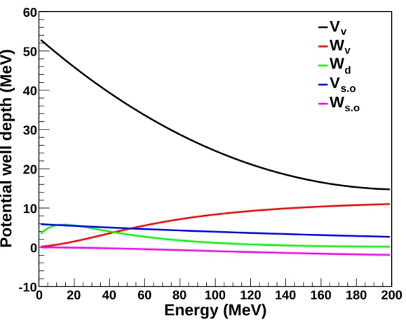
2.2 Functional form of the optical model potential well depths . . . 51
2.3 Level densities for 20Ne and 40Ar calculated using the
constant temperature and Fermi gas models . . . 58
3.1 TUNL floorplan . . . 69
3.2 Direct Extraction Negative Ion Source (DENIS II) . . . 71
3.3 Tandem Van de Graaff accelerator schematic . . . 75
3.4 Deuterium gas cell for neutron production . . . 79
3.5 The TUNL time-of-flight setup . . . 82
3.6 The scattering targets mounted in the NTOF beam line . . . 84
3.7 Schematic of the NTOF detector shielding . . . 86
3.8 Schematic of the TUNL time-of-flight data acquisition and electronics . . . 89
4.1 A 137Cs spectrum for the four-meter detector . . . . 93
4.2 A PSD spectrum for the four-meter detector . . . 94
4.3 TDC spectrum before and after threshold and PSD cuts . . . 96
4.4 Floor monitor TOF spectrum . . . 98
4.5 Normalized SAMPLE IN, SAMPLE OUT and DIFF TOF spectra for a neon target . . . 100
4.6 Normalized SAMPLE IN, SAMPLE OUT and DIFF TOF spectra for polyethylene and carbon targets . . . 101
4.7 TOF difference spectrum for neon . . . 102
4.8 Detector efficiencies for the four-meter and six-meter detectors . . . 107
4.9 Multiple scattering and finite geometry corrections for neon . . . 111
4.9 Multiple scattering and finite geometry correction for argon . . . 112
4.10 Data and Legendre polynomial fits of the differential elastic scattering cross section of neutrons from natNe . . . . 116
4.12 Optical-model calculations of the differential elastic scattering cross section of neutrons from natNe at
5.0 and 8.0 MeV . . . 122
4.13 Optical-model calculations of the differential elastic scattering cross section of neutrons from natAr at 6.0 and 14.0 MeV . . . 124
4.14 Optical-model calculations of the differential elastic scattering cross section of neutrons from natAr from 0.5 to 20 MeV . . . 125
4.15 Optical-model calculations of the differential elastic scattering cross section of neutrons from natNe from 3 to 10 MeV . . . 127
5.1 Schematic of the GEANIE beam line at LANSCE . . . 131
5.2 The beam pulsing structure of the LANSCE neutron beam . . . 132
5.3 The LANSCE in-beam fission ionization chamber. . . 134
5.4 Detector placements within the GEANIE array . . . 137
5.5 A block diagram of the GEANIE detector circuit . . . 141
6.1 TDC spectrum for a GEANIE HPGe detector summed over all neutron energies . . . 149
6.2 TOF spectrum for a GEANIE HPGe detector summed over all neutron energies . . . 150
6.3 Self-triggered TDC range for 238U fission chamber data . . . 151
6.4 Example energy calibration for a GEANIE coaxial HPGe detector . . . 152
6.5 En vs Eγ histograms for argon and neon sample data . . . 154
6.6 Argon-sample γ-ray spectra selected for different neutron energy windows . . . 155
6.7 Neon-sample γ-ray spectra selected for different neutron energy windows . . . 156
6.9 An example GEANIE HPGe detector efficiency curve . . . 164
6.10 Simulated efficiency curves for GeQ detector using a
point source and argon gas cell . . . 165
6.11 The simulated efficiency of the GeQ detector for 1000 keV γ rays
distributed in 2-mm thick rings relative to a point source . . . 167
6.12 A sample ADC spectrum for the 238U fission chamber summed
over all neutron energies from 1 to 100 MeV . . . 168
6.13 The neutron flux per micropulse measured with the fission
chamber upstream from the GEANIE array . . . 170
6.14 The angular distribution of γ rays for the E2 2+ →0+ first
excited states in 40Ar and 20Ne . . . . 173
6.15 Partial γ-ray production cross section for the 846.8-keV 2+ →0+
transition in 56Fe . . . . 175
6.16 Partial γ-ray cross sections for40Ar(n, n0γ)40Ar . . . . 176
6.17 Partial γ-ray cross sections for measured transitions in
39Ar(n,2nγ)40Ar . . . . 179
6.18 Partial γ-ray production cross section for the 1633-keV
2+ →0+ transition in 20Ne . . . . 181
6.19 Partial γ-ray production cross section for the 1275-keV
2+ →0+ transition in 22Ne . . . 182
7.1 Argon γ-ray spectra for neutron energies of 2 to 20 MeV
in the 76Ge 0νββ regions of interest. . . . . 185
7.2 TALYS calculations for the 2+→2+ Eγ = 2050.5 keV or
4+ →2+ E
γ = 2054 keV transitions in40Ar . . . 186
7.3 Upper limits for natAr(n, xnγ) reactions. . . 187
7.4 A comparison of the original G4NDL 3.14 cross sections for
22Na and modified cross sections for natNe at 5.0 and 8.0 MeV. . . . 190
7.5 A comparison of the original G4NDL 3.14 elastic scattering
7.6 A comparison of the original G4NDL 3.14 cross sections
and modified cross sections for 40Ar at 6.0 and 14.0 MeV. . . . 192
7.7 A comparison of the original G4NDL 3.14 elastic scattering
cross section for and modified cross section for 40Ar . . . 193
7.8 A simple model geometry representing the MiniCLEAN
detector to be used for neutron background studies . . . 195
7.9 Simulated neutron energy and nuclear recoil energy spectra
for a MiniCLEAN fiducial volume made from liquid argon . . . 198
7.10 Simulated neutron energy and nuclear recoil energy spectra
for a MiniCLEAN fiducial volume made from liquid neon . . . 199
7.11 Ratio of the argon elastic scattering cross section to the
γ-ray production cross section. . . 202
7.12 Ratio of the neon elastic scattering cross section to the
γ-ray production cross section. . . 203
A.1 The 238U decay chain . . . 209
List of Tables
1.1 Some physical properties of Ne, Ar and Xe . . . 17
1.2 Neutrino mixing angles and mass splittings . . . 24
1.3 Current and proposed ββ0ν experiments. . . 30
2.1 Neutron global optical model parameters . . . 50
2.2 Default parameters used for level-density calculations for argon and neon . . . 57
2.3 Weisskopf estimates for electric and magnetic transition rates . . . 62
3.1 Deuterium gas cell pressures and neutron energy spreads . . . 78
3.2 Description of the gas targets . . . 81
3.3 Description of the polyethylene and carbon scattering targets . . . 81
3.4 Properties of the TUNL time-of-flight liquid scintillator detectors . . . 83
4.1 Selected n−p scattering cross sections used for data normalization . . . 104
4.2 Systematic and statistical uncertainties for NTOF σ(θ) data . . . 113
4.3 The total elastic and zero-degree cross section for natAr(n, n)natAr from optical-model calculations, fits and data . . . 126
4.4 The total elastic and zero-degree cross section for natNe(n, n)natNe from optical-model calculations, fits and data. . . 126
5.1 Description of foils in the fission chamber . . . 135
5.2 Detector placements within the GEANIE array . . . 138
6.2 Prominent background γ-ray lines in GEANIE spectra . . . 157
6.3 GEANIE systematic and statistical uncertainties . . . 174
6.4 Summary of the measured γ-ray production cross sections for argon. . . 180
6.5 Summary of the measured γ-ray production cross sections for neon. . . 181
7.1 Upper limits for natAr(n, xnγ) reactions . . . . 186
7.2 Calculation of the 238U- and 232Th-induced natB(α, n) yields in borosilicate PMT glass using a simple MiniCLEAN geometry model . . . 196
7.3 Results for simulated PMT neutrons in a simple MiniCLEAN detector . . . 200
8.1 Summary of the elastic scattering cross sections for argon and neon . . . 205
B.1 Measured differential cross sections for the scattering of 5.0-MeV neutrons from natNe. . . . 211
B.2 Measured differential cross sections for the scattering of 8.0-MeV neutrons from natNe. . . . 212
B.3 Measured differential cross sections for the scattering of 6.0-MeV neutrons from natAr. . . 213
B.4 Measured differential cross sections for the scattering of 14.0-MeV neutrons from natAr. . . 214
B.5 Fit parameters for natNe 5.0-MeV scattering data. . . . 215
B.6 Fit parameters for natNe 8.0-MeV scattering data. . . . 215
B.7 Fit parameters for natAr 6.0-MeV scattering data. . . 216
B.8 Fit parameters for natAr 14.0-MeV scattering data. . . . . 216
B.10 Neutron surface optical model parameters for natNe. . . 217
B.11 Neutron spin-orbit optical model parameters for natNe. . . . 218
B.12 Neutron volume optical model parameters for natAr. . . . 218
B.13 Neutron surface optical model parameters for natAr. . . . 218
B.14 Neutron spin-orbit optical model parameters for natAr. . . . . 219
C.1 40Ar(n, n0γ)40Ar 2+→0+ Eγ = 1461 keV . . . 220
C.2 40Ar(n, n0γ)40Ar 0+→2+ E γ = 660 keV . . . 221
C.3 40Ar(n, n0γ)40Ar 2+→0+ Eγ = 2524 keV . . . 221
C.4 40Ar(n, n0γ)40Ar 2+→2+ E γ = 1063 keV . . . 221
C.5 40Ar(n, n0γ)40Ar 4+→2+ E γ = 1432 keV . . . 222
C.6 40Ar(n, n0γ)40Ar 2+→2+ Eγ = 1747 keV . . . 222
C.7 40Ar(n,2nγ)39Ar 3/2− →7/2− E γ = 1267 keV . . . 222
C.8 40Ar(n,2nγ)39Ar 3/2+ →3/2− Eγ = 250 keV . . . 222
C.9 20Ne(n, n0γ)20Ne 2+→0+ E γ = 1633 keV . . . 223
Chapter 1
Background and Motivation
1.1
Dark Matter
Dark matter is a type of matter that accounts for about one quarter of the
mass-energy in the universe. Unlike the matter made up of protons, neutrons and electrons,
dark matter neither emits nor absorbs detectible amounts of electromagnetic radiation.
Because it is not visible, its existence must be inferred from its gravitational interaction
and influence on the observed large-scale structure of the universe. This section will
describe the current evidence for dark matter, candidates for dark matter, and the
current status of experimental techniques for its direct detection.
1.1.1
Dark Matter on Galactic Scales
The existence of dark matter was first postulated by Zwicky in 1933 [Zwi33], who
calculated that the gravitational mass of galactic clusters must be much greater than
expected from their luminosity. Since then, the existence of dark matter has been
verified in a variety of different ways, the first of which was from the measurements of
in a stable Keplerian orbit is
v(r) = r
GM(r)
r , (1.1)
whereM(r) is the mass inside the orbit at a particular radiusr. Therefore, forroutside
the visible part of the galaxy, the rotational velocity should scale as v(r) ∝ 1/√r. It was observed however, that the rotational velocity was greater than expected if mass
tracks light. In most galaxies, it was found that v becomes approximately constant to
measurable values of r. This implies that there is a halo comprised of non-luminous
matter withM(r)∝r and mass density ρ(r)∝1/r2.
Dynamical evidence for dark matter can be inferred from motion of galaxies relative
to one another, which was found to be slower than Hubble’s law would predict. These
“peculiar velocities” allow for estimates of galactic masses based on the assumption
that gravitational interactions are responsible for their motions. Analyses of peculiar
velocities indicated that the total matter density of the Universe must be greater than
the value that is permitted by the standard model of Big-Bang nucleosynthesis [Lid99].
The conclusion is that not only is the Universe composed of dark matter, but at least
some of it takes a non-baryonic form.
Observations of x-rays from hot gas in galaxy clusters provide more evidence for
dark matter. X-ray maps show that within galaxy clusters, there is more matter in the
gas than in all of the galaxies put together. After accounting for the hot gas as well as
the possibility of stars too faint to detect or with insufficient material to initiate nuclear
burning, it can be determined that clusters contain mostly dark matter [Lid99].
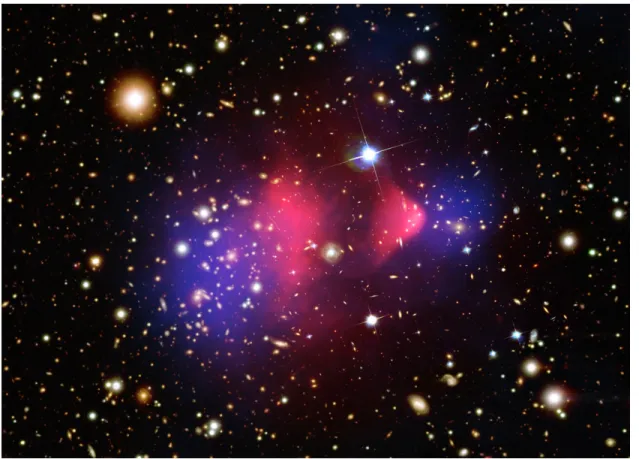
One particularly interesting example is the bullet cluster shown in Fig. 1.2. The
Magellan Telescopes mapped the location of the mass in the bullet cluster through
Figure 1.2: Composite image of the matter in the bullet cluster. The dark matter (blue) trails the luminous matter (red) following the collision of two galaxy clusters. Composite image from NASA [NAS06].
the luminous matter taken from the Chandra X-ray Observatory [Mar05]. The
result-ing structure shows two clusters of galaxies passresult-ing through one another. One possible
interpretation is that the luminous matter, shown in red, interacts with luminous
mat-ter in the other clusmat-ter, slowing it down, whereas the dark matmat-ter, shown in blue,
passes directly through. The result is that each galaxy cluster is separated into two
components; the luminous matter trailing the dark matter.
1.1.2
Modern Cosmology
Modern cosmology has been successful in describing many areas of observational
that contains a cosmological constant, Λ, as well as cold dark matter (CDM). This
model, which contains only a few parameters, can describe many features of the
Uni-verse today, including the cosmic microwave background (CMB) [Hu97], the large-scale
structure of the Universe, the light-element abundances, and the accelerating expansion
of the Universe [Lid99].
The model contains density parameters, Ωi, which determine the abundance of a
specific substance in the Universe of species i, and are given as
Ωi ≡
ρi
ρc
, (1.2)
where ρi is the density of species i and ρc is the critical density, given in terms of
an expansion parameter (the Hubble constant, H0 = 100 h km s−1 Mpc−1, where
h= 0.72±0.03 [Ber12]) as
ρc=
3H02
8πG. (1.3)
To show how these parameters fit into the model, we start with Einstein’s theory
of general relativity, which states how the presence of matter curves space-time. The
Friedmann equation, a simple form of Einstein’s equations [Ein16] is given as
H02 = 8πG 3 ρ−
k
a2, (1.4)
where ρ is the energy density, which can have a number of different subcomponents,
k is the curvature constant, and a is a scale factor. Following Ref. [Bah99], we will
consider a model which contains matter, m, curvature,k, and a cosmological constant,
Λ. The cosmological constant can be thought of as the energy density of empty space,
or “dark energy”. It is speculated to be responsible for the observed acceleration of the
right hand side of Eqn. 1.4 are given by
Ωm = 8πGρm/3H02, (1.5)
ΩΛ = 8πGρΛ/3H02, (1.6)
Ωk=−k/(aH0)2. (1.7)
Dividing both sides of Eqn. 1.4 byH2
0 gives the sum rule:
1 = Ωm+ Ωk+ ΩΛ. (1.8)
Inflationary theory [Gut81] and analysis of the CMB [Hin09] appear to suggest
the universe is flat (Ωk = 0). The ΛCDM model contains four basic parameters:
Ωm = 1/3, ΩΛ = 2/3, Ωk = 0, and H0. The mass-energy breakdown according to the
current ΛCDM model is a mixture of ∼ 70% dark energy, ∼ 25% dark matter and ∼
5% normal matter (electrons, protons, neutrons and neutrinos) [Lid99].
Quantitative information on the total amount of matter in the universe may be
extracted from analysis of the CMB, large-scale structure, and other observations. The
CMB spectrum is described by a blackbody function with T = 2.725 K.
Temper-ature angular anisotropies in the CMB at the 10−5 level were first discovered with
the COBE satellite [Smo92]. These data were improved upon by NASA’s Wilkinson
Microwave Anisotropy Probe (WMAP) [Ben03, Hin09] and several ground-based
Figure 1.3: The observed power spectrum of CMB anisotropies from WMAP. From Ref.[Lar11].
The observed anisotropies put stringent constraints on various cosmological
param-eters, including dark matter. The temperature anisotropies are expanded as
∆T
T (θφ) =
+∞
X
l=2 +l
X
m=−l
almYlm(θφ), (1.9)
whereYlm(θφ) are the spherical harmonics. The variance Cl of alm is given by
Cl ≡
|alm| 2
≡ 1
2l+ 1
l
X
m=−l |alm|
2
. (1.10)
The information in the CMB maps is usually compressed in a power spectrum,
which gives the behavior of ∆T as a function of l (see Fig. 1.3).
The monopole terma00 determines the mean CMB temperature,T = 2.725 K. The
higher order multipoles represent perturbations in the density of the early universe.
The first peak’s position, centered around l = 200, is sensitive to curvature, and is in
good agreement with a flat Universe [Hin09]. The series of peaks in the power spectrum,
early Universe [Eis05], is sensitive to the energy density ratio of dark matter to radiation
in the Universe [Hu96a, Hu96b, Hu12]. A standard set of cosmological parameters
obtained using the CMB data can be found in Ref.[Ber12]. The total matter density
is Ωmh2 = 0.133 ± 0.066 and the baryon density is Ωbh2 = 0.0227 ±0.0006. The
measurement of Ωbh2 using the CMB data is in good agreement with the observed light
element abundances and the standard model of Big-Bang nucleosynthesis [Lid99].
1.1.3
Dark Matter Properties
Because Ωb << 1, it is clear that baryons cannot account for all of the mass-energy
in the Universe. In fact, using the parameters from the CMB, one finds that
non-baryonic matter constitutes the majority of the matter density in the Universe with a
density of Ωnbmh2 = 0.110±0.006 [Ber12]. Additionally, the optically luminous matter
density is Ωlumh−1 ≈ 0.0024 [Fuk04], so the baryon density is much greater than the
luminous matter density. This implies that most of the baryons in the Universe are
optically dark, probably in the form of a diffuse intergalactic medium [Cen99]. It is
possible, however, that some of the baryonic matter could contribute to dark matter.
Popular candidates for baryonic dark matter include MAssive Compact Halo Objects
(MACHOs) [Pac86, Gri91] or cold molecular gas clouds [DeP95]. Because the total
matter density is Ωm ∼ 0.3, we can conclude that most matter in the Universe is not
only optically dark, but is also non-baryonic. The analysis of structure formation in the
universe suggests that dark matter should also be “cold” (non-relativistic) [Ber10]. This
is consistent with the upper bound on the possible contribution from light neutrinos.
Because neither baryons nor neutrinos can be all of the dark matter, it is necessary
to postulate new kinds of particles not currently found within the Standard Model,
assuming that the general relativistic principles underlying the cosmological models
conditions: (a) they must be stable on cosmological timescales, otherwise they would
have decayed, (b) they must interact weakly or not at all with electromagnetic radiation,
otherwise they would not be optically dark, (c) they must interact weakly or not at all
with “normal” matter, (d) they must yield the correct relic density.
1.1.4
Weakly Interacting Massive Particles
When considering the criteria for a non-baryonic cold dark matter candidate, a
well-motivated theoretical and experimental choice appears to be a Weakly Interacting
Mas-sive Particle (WIMP), denoted by χ. The fact that annihilation cross sections on the
weak scale lead to the correct relic abundance, sometimes referred to as the “WIMP
miracle”, was first noticed in the late 1970s [Hut77, Lee77]. This first proposed WIMP,
a massive neutrino, is currently not well-motivated by particle physics because it
re-quires a large mass splitting between the three known neutrinos [Pri88].
Among the proposed WIMP candidates, the currently best motivated choice
ap-pears to be the lightest superparticle (LSP) in supersymmetric (SUSY) models [Mar11,
Jun96]. SUSY models describe a complete symmetry between fermions and bosons and
have many interesting features that make them attractive. Specifically, SUSY solves
di-vergence problems in calculating certain Standard Model interactions, such as the Higgs
mass correction. It also provides a framework to unify particle physics and gravity, and
may explain the origin of the large differences between the electroweak scale, v =
(√2GF)1/2 ≈246 GeV and the Planck scale, Mp ≈1019 GeV [Dim81, Sus84, Ber12]. If
the SUSY solution is correct, supersymmetric particles could be observed with the next
generation of particle accelerators, such as the Large Hadron Collider (LHC) [CER12].
A subset of supersymmetric theories, the Minimal Supersymmetric Standard Model
(MSSM) contains the smallest amount of additional information to fully describe all
MSSM models contain a conserved multiplicative quantum number, called R-parity,
defined as
R ≡(−1)3B+L+2s, (1.11)
where B is the baryon number, L is the lepton number and s is the spin. All of
the Standard Model particles have R = 1 and all superparticles have R = −1. As a consequence ofR-parity conservation, superparticles can only decay into an odd number
of superparticles and the LSP can only be destroyed by pair annihilation. Because dark
matter has no electromagnetic interactions, a WIMP LSP must have no charge, ruling
out several candidates. The stability of the LSP makes it an excellent WIMP candidate,
since they would have been produced copiously during the Big Bang and would still be
present today.
It is possible that the dark matter is not a WIMP, nor does it need to be one specific
type of particle. Further discussion on some of the more exotic forms of dark matter
can be found in Refs.[Ber05, Ber00] and references therein. One particularly interesting
non-WIMP candidate for dark matter is the axion, which was postulated to solve the
“strong CP” problem in quantum chromodynamics (QCD) [Pec77b, Pec77a]. Even though axions would be light, they would still be classified as cold dark matter because
they would be produced non-thermally [Ber12]. Although the axion is a perfectly viable
dark matter candidate, we will restrict our further discussion mainly to the WIMP.
1.1.5
Methods for WIMP Detection
In some detectors for nuclear physics experiments, such as scintillators, particle
de-tection is accomplished by the transfer of energy to electrons in a detector. Whereas
charged particles and photons may interact directly with the atomic electrons, other
often detected by the transfer of kinetic energy to a nucleus, which can then produce
ionization. Dark matter particles are difficult to detect because they are both neutral
and weakly interacting. Methods for detecting WIMP dark matter can be classified as
“direct” or “indirect”. Direct methods are those in which all interactions take place in a
terrestrial apparatus. These methods and experiments will be discussed in detail in the
following sections. Indirect methods are those in which the primary interaction happens
outside the Earth and produces observable particles that can be detected. For example,
positrons may be created through WIMP annihilation in the Milky Way [Jun96]. Both
PAMELA [Adr09] and the Fermi Large Area Telescope [Abd09] have observed an
ex-cess of high-energy positrons compared to conventional astrophysical models [Mos98].
Although these observations are interesting, they cannot rule out astrophysical sources
such as pulsars [Ato95] as a source of the observed excess.
Particle colliders may also be used to look for supersymmetric dark matter.
Specif-ically, the Large Hadron Collider (LHC) is a proton-proton collider that has two large,
general purpose experiments called ATLAS [Aad08] and CMS [Ado08], which are being
used to search for physics beyond the Standard Model. Energetic collisions at the LHC
may produce a variety of supersymmetric particles. Squarks and gluinos, which are the
superpartners of the Standard Model quarks and gluons will be produced according to
their masses and strong couplings. Considering a model in whichR-parity is conserved,
they will each cascade to the LSP, which will escape the detector. The LSP can be
therefore be characterized by the “missing energy” in the event. The disadvantage of
such searches is that the signatures are model dependent [Ber10].
1.1.6
Direct Detection of WIMP Dark Matter
The basics of a direct WIMP search are very simple in principle. WIMPs are
direct detection of WIMPs is possible by searching for the nuclear recoil from a
pu-tative WIMP-nucleus scatter. For WIMP masses in the 10 GeV to 1 TeV range, the
nuclear recoil energy will be less than about 100 keV. Because any particle can scatter
from an atomic nucleus, fast neutrons can also deposit energy in these detectors. These
scattered neutrons are indistinguishable from WIMPs and are therefore potentially the
most dangerous source of background. However, it is interesting to note that the
ulti-mate sensitivity of direct detection experiments to WIMPs in this mass range will be
limited by coherent nuclear scattering from solar neutrinos.
The shape of the nuclear recoil spectrum depends on the WIMP velocity
distribu-tion, which is usually taken to be a Maxwellian distribution with an average of 220
km/s. The differential energy spectrum is expected to be a featureless and smoothly
decreasing exponential function [Lew96]. The expected rate in a direct detection
ex-periment is given approximately by Ref.[Ber05] as
R ≈X
i
Ni
ρχ
mχ
hσiχi. (1.12)
This rate depends on the number of nuclei in the detector, Ni, of species ifrom which
a WIMP could scatter, the local WIMP density ρχ, the WIMP mass mχ and the
WIMP-nucleus interaction cross sectionhσiχi. Based on galactic modeling, Ref.[Kam98]
estimated the local dark matter density to be ρlocal
DM ≈ 0.3 GeV cm
−3. This essentially
leaves the mass and cross section of the WIMP as unknowns. For this reason, the
experimental observable, which is the scattering rate as a function of nuclear recoil
energy, is usually expressed as a contour in the WIMP cross section - WIMP mass plane.
At low WIMP masses, the sensitivity decreases due to experimental energy thresholds.
At high WIMP masses, the sensitivity decreases because the rate is proportional to
1/mχ. From these considerations, direct detection experiments will be more sensitive
The WIMP scattering cross section also depends on the nature of the couplings.
WIMP scattering is usually discussed in the context of dependent (SD) and
spin-independent (SI) couplings. Because SD interactions depend on a nuclear spin factor
J(J+1) rather than the number of nucleons, little is gained from using a heavier target.
On the other hand, SI cross sections scale approximately as the square of the nuclear
mass numberA. It is therefore preferable to use higher-mass nuclei as targets for these
types of experiments.
1.1.7
Direct Detection Experiments
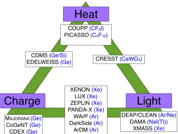
There are many direct dark matter detection experiments that use of a variety of
dif-ferent technologies including detection via ionization, scintillation, phonons, or some
combination. A selection of current direct dark matter detection experiments is
illus-trated in Fig. 1.4. For detailed descriptions of these experiments, the reader is referred
to Refs.[Ber12, Ber10] and references therein. Fig. 1.5 shows a selection of current
experimental results along with selected theoretical predictions and next generation
experiment’s projected sensitivities.
There are currently several experiments that have claimed a result consistent with
WIMPs. The DAMA collaboration operated up to 250 kg of NaI(Tl) detectors at the
Laboratori Nazionali del Gran Sasso (LNGS), near L’Aquila, Italy. They search for an
annual modulation in their signal as a consequence of the Earth’s rotation around the
Sun with respect to the solar system’s rotation around the galaxy. A higher WIMP
flux is expected around June 2, when the two velocities are in the same direction, and
a smaller flux around December 2, when the two velocities are in opposite directions.
They have reported an observed annual modulation of their signal with the expected
period and phase at an 8.9 σ level. The red regions in the plot show two possible
Heat
Charge
Light
M
AJORANA(Ge)
CoGeNT
(Ge)
CDEX
(Ge)
XENON
(Xe)
LUX
(Xe)
ZEPLIN
(Xe)
PANDA-X
(Xe)
WArP
(Ar)
DarkSide
(Ar)
ArDM
(Ar)
DEAP/CLEAN
(Ar/Ne)
DAMA
(NaI(Tl))
XMASS
(Xe)
CDMS
(Ge/Si)
EDELWEISS
(Ge)
CRESST
(CaWO
4)
COUPP
(CF
3I)
PICASSO
(C
4F
10)
about 6 to 10 GeV. The dark red regions correspond to the DAMA data if there was a
significant ion channeling effect [Ber07].
The CRESST experiment [Ang11] uses both the phonon and scintillation signal from
cryogenic CaWO4. A recent analysis of their data showed an excess compatible with
WIMPs, although their signal is present in a large background. The green regions in
Fig. 1.5 show the results of a maximum likelihood analysis which provides two possible
solutions at the 4σ level corresponding to WIMP masses of about 12 and 25 GeV.
There is considerable tension with these results and the compatibility with the null
observations from several other experiments. The CDMS [Coo10] and XENON100 [Apr11]
experiments, along with the 2010 CoGeNT analysis [Aal11] seem to rule out both the
CRESST and DAMA results. The next generation of WIMP dark matter direct
detec-tion experiments should provide significant insight into this problem. Projected
sensi-tivities of these experiments will probe cross sections as low as 10−47 cm2 for WIMP
masses on the 10 to 1000 GeV range, testing many of the SUSY model predictions.
A selection of future experiment’s projected sensitivities are shown as dashed curves
in Fig. 1.5. Experiments with very low energy thresholds such as the Majorana
Demonstrator(Section 1.2.5) will be sensitive to lighter WIMP masses.
1.1.8
Noble Liquids for WIMP Detection
Of particular relevance to this dissertation, several of the current and next generation
large-scale detectors designed to search for WIMP dark matter will make use of large
volumes of liquified noble gas (LNe, LAr, LXe). Noble liquids are excellent scintillators
and have a large ionization yield in response to the passage of radiation. In addition,
the relative low cost and ease of scalability make them attractive target materials
for WIMP searches. These experiments will search for the scintillation light, and in
WIMP Mass [GeV/c
2
]
Cross
section [cm
2
] (normalised to nucleon)
120821120501
http://dmtools.brown.edu/ Gaitskell,Mandic,Filippini
10
010
110
210
310
4810
4610
4410
4210
4010
38120821120501
XENON1T, projection 2009, SI
Ruiz de Austri et.al., 2006, CMSSM Markov Chain Monte Carlos: 95% contour, DEAP CLEAN, projection 2007, 1,000kg FV, SI
DEAP CLEAN, projection 2007, 150kg FV, SI XENON100, 2011, 100.9 live days of data, SI
CDMS II (Soudan), 2004 to 2009 combined all data from Soudan, SI CRESST II, 2011, 730kg days, 2 sigma allowed region, SI pt. 1 DAMA/LIBRA, 2008, no ion channeling, 3sigma, SI
DAMA/LIBRA, 2008, with ion channeling, 3sigma, SI
CRESST II, 2011, 730kg days, 2 sigma allowed region, SI pt. 2 CoGeNT, 2010, SI
DATA listed top to bottom on plot
Table 1.1: Some relevant physical properties of Ne, Ar and Xe. Excimer lifetimes from Refs.[Lip08, Nik08, Hit83].
Property Ne Ar Xe
Atomic number 10 18 54
Mean atomic mass 20.2 40.0 131.3
Boiling point Tb at 1 atm (K) 27.1 87.3 165.0
Liquid density at Tb (g/cm3) 1.12 1.40 2.94
Scintillation wavelength (nm) 78 128 178 Singlet lifetime (ns) <18.2±0.2 7.0±1.0 4.3±0.6 Triplet lifetime (ns) 14900±300 1600±100 22.0±2.0
WIMP-nucleus scatter.
Scintillation light is generated in noble gases as a result of Ne, Ar or Xe atoms,
de-noted by R, interacting with ionizing radiation where an excited dimer R∗2is formed [Kub77,
Apr05]. The scintillation light has two decay components due to de-excitation of the
singlet and triplet states of the excimer R∗2 → 2R +hν, where hν denotes a vacuum-ultraviolet (VUV) photon emitted in the process. Whereas the scintillation pulse shape
from nuclear recoils shows both a fast and a slow component from the de-excitation of
singlet and triplet states, respectively, an electronic recoil produces only a slow
compo-nent [Hit83]. The difference in the scintillation response to different types of radiation
becomes the basis for pulse shape discrimination (PSD). This is most effective in LAr
and LNe where the time separation between the two decay components is large. Some
of the relevant physical properties of Ne, Ar and Xe are shown in Table 1.1.
Noble gas detectors for dark matter searches may be divided roughly into two classes:
those that use both the scintillation and ionization channels and those that use the
scintillation channel only. The breakdown of these experiments including their detector
target material can be seen in Fig. 1.4.
Time Projection Chambers (TPCs) make use of both the ionization and scintillation
signal. An event within the liquid volume of the TPC will create both ionization
drift under the influence of an external electric field into a gas volume where they
produce a second scintillation signal proportional to the ionization yield [Dol70, Bol99,
Bol06], referred to as S2. The ratio S2/S1 will be higher for an electronic recoil
which produces a greater ionization yield than for a nuclear recoil. Because WIMPs
or neutrons produce nuclear recoils, whereas β and γ rays produce electronic recoils,
this becomes the basis for background discrimination. An ArTPC has the advantage
over a XeTPC in that PSD may be used in addition to S2/S1. The disadvantages
of the ArTPC are the lower mass number and because the scintillation wavelength is
small compared to Xe, a wavelength shifter must be used for the efficient detection by
commercial photomultiplier tubes (PMTs).
The DEAP/CLEAN Experimental Program
Single phase noble liquid detectors search for WIMPs using the scintillation channel
only. The Dark matter Experiment with Argon and Pulse shape discrimination (DEAP)
and proposed Cryogenic Low Energy Astrophysics with Noble gases (CLEAN)
exper-iments are based on LAr and LNe detectors for dark matter and pp solar neutrino
detection [Bou04]. Both materials have excellent scintillation light yields, are
trans-parent to their own scintillation light, and allow pulse shape discrimination to separate
electronic and nuclear recoils [Lip08, Nik08]. The MiniCLEAN detector is a 500 kg
(∼100 kg fiducial mass) prototype to be built at SNOLAB, located in Sudbury, On-tario, which will operate interchangeably with LAr and LNe [McK07]. The experiment
will first run with LAr to be followed by operation with LNe. Because the WIMP
scattering cross section scales as A2, the event rate of a potential signal can be
com-pared between the different phases to verify a potential WIMP signal. The detector
Figure 1.6: Schematic view of the MiniCLEAN (left) and DEAP-3600 (right) detectors. The MiniCLEAN inner target has a diameter of about 45 cm. The DEAP-3600 inner target will be about twice the diameter of MiniCLEAN to accommodate a larger fiducial mass. Figures from the DEAP/CLEAN collaboration (deapclean.org).
of the detector will be viewed by 92 PMTs immersed in the cryogenic liquid. The
pri-mary scintillation light will be absorbed by a tetra-phenyl butadiene (TPB) wavelength
shifter, reemitted in the visible range, and will be transported to the PMTs via acrylic
lightguides. Additionally, a 3600 kg LAr detector, called DEAP-3600, is being deployed
at SNOLAB [Bou08]. The detector will have a fiducial mass of approximately 1000 kg
viewed by 266 PMTs. A schematic view of the MiniCLEAN and DEAP-3600 detectors
is shown in Fig. 1.6. The longer-term goal for the DEAP/CLEAN collaboration is to
1.2
Neutrino Masses and Mixings
1.2.1
Neutrino History
Early physics experiments had shown that α particles were emitted at well-defined
energies, but physicists were puzzled when they found that β particles were emitted
with a continuous energy distribution. A new particle was first postulated by Pauli
in a letter to the attendees of a physics conference in T¨ubingen, Germany in 1930
as a “desperate remedy” to conserve energy and angular momentum in the β-decay
process [ETH]. This new particle would be electrically neutral to conserve charge, and
would have spin 12 to conserve angular momentum. It also must not interact strongly
with matter so that it would not be detected along with the electron. Later, in a letter
to Fred Reines, Fermi called this particle the neutrino. Nuclear beta decay can be written as
A
ZXN →AZ+1 XN−1+e−+ ¯νe, (1.13)
where the neutrino ¯νe is actually an anti-neutrino so the final state contains a lepton
anti-lepton pair. Following Pauli’s neutrino hypothesis, Fermi developed the formal
theory ofβ decay in 1934 [Fer34], which has since evolved into the standard model of
electroweak interactions.
The neutrino remained elusive for more than two decades before it was
discov-ered in 1956 by Reines and Cowan using anti-neutrinos produced from a nuclear
reac-tor [Rei53, Cow56]. Less than ten years later, a new discovery was made at Brookhaven
National Laboratory (BNL) showing the neutrinos produced with muons were different
than neutrinos produced with electrons [Dan62]. Following this discovery, these
neutri-nos were referred to as “electron-neutrineutri-nos” (νe) and “muon-neutrinos” (νµ). In 1989,
(LEP) at CERN showed that there were three families of light, weakly-interacting
neu-trinos [DeC89]. In 2000, the DoNuT Experiment at Fermilab confirmed the existence
of a “tau-neutrino”(ντ) [Kod02].
1.2.2
Neutrino Masses and Mixings
During the 1950s and 1960s, attempts to observe neutrinos from the sun were pioneered
by Davis and Bahcall [Bah64, Dav64]. The famous Homestake neutrino experiment
de-tected solar neutrinos in 1968 with a flux of only about one third of what was predicted
from solar models [Cle98]. This discrepancy was known as the “solar neutrino
prob-lem”. A proposed solution to this problem was that neutrinos can change in flavor
on macroscopic length scales provided that they have mass and their states of definite
mass (ν1,ν2,ν3) are not the same as their flavor states (νe,νµ,ντ). This difference
be-tween flavor and mass eigenstates lead to the phenomenon of neutrino oscillations. In
this scenario, the three known neutrino flavor eigenstates can be connected with the
mass eigenstates through the Pontecorvo-Maki-Nakagawa-Sakata (PMNS) matrix Uαi
as [Pon68, Mak62]
|ναi=
X
i
Uαi|νii, (1.14)
where |ναi represents a neutrino with definite flavor, α, and |νii represents a neutrino
with definite mass,i.
Considering a hypothetical two-neutrino scenario, the mixing can be described by
a 2×2 matrix, given by
U2ν =
cosθ sinθ
−sinθ cosθ
. (1.15)
flavor state β can be calculated to be [Bil78]
Pαβ = sin2(2θ) sin2
1.27(m 2
i −m2j)L
E
, (1.16)
which describes periodic neutrino oscillations. The angleθdetermines the amplitude of
the oscillation, i.e. the amount of mixing between flavor states α and β. The quantity
Lis the distance the neutrino has traveled in km,E is the neutrino energy in GeV, and
mi,j are the neutrino masses in eV. The quantitym2i −m2j determines the frequency of
the oscillation.
Extending this to the three-neutrino scenario, a common parameterization of the
mixing matrix motivated by experimental observables is given by
U =
Ue1 Ue2 Ue3
Uµ1 Uµ2 Uµ3
Uτ1 Uτ2 Uτ3 =
1 0 0
0 c23 s23
0 −s23 c23
c13 0 s13e−iδ
0 1 0
−s13e−iδ 0 c13
c12 s12 0
−s12 c12 0
0 0 1
eiα1/2 0 0
0 eiα2/2 0
0 0 1
, (1.17)
where sij ≡ sin(θij) and cij ≡ cos(θij). The mixing matrix can be described by three
angles and one complex phase, δ, which is non-zero only if neutrino oscillations
vi-olate CP symmetry. The phases α1 and α2 affect only Majorana particles [Avi08] (see Section 1.2.3). Although the probabilities Pαβ in the real three-neutrino scenario
may depend on all of the observable parameters that characterize U, the approximate
While neutrino oscillations indicate that neutrinos have mass, the experiments are
sensitive only to the absolute value of the differences in the squares of the neutrino
masses, ∆m2
ij ≡ |m2i − m2j|. However, a lower limit on the absolute value of the
neutrino mass scalemscale =
√
∆m2 can be determined. Neutrino oscillations were first
discovered in atmospheric neutrinos by the Super-Kamiokande collaboration in 1998
[Fuk98]. These results can be interpreted as nearly maximal mixing between the νµ
andντ neutrinos. This mixing, known as atmospheric mixing, gives one of the angles in
the PMNS matrix,θ23. This angle has since been constrained further by searches forνµ
disappearance in accelerator-producedνµ beams, specifically by the K2K [Ahn06] and
MINOS [Ada12] experiments. The corresponding ∆m2 implies a neutrino mass scale of
about 50 meV. Results from the Sudbury Neutrino Observatory (SNO) provided a direct
solution to the “solar neutrino problem” discussed above by showing ve’s produced in
the sun underwent flavor change affected by solar matter [Ahm01, Wol78]. The solar
mixing angle,θ12, and associated mass splitting was determined from SNO [Aha08] and
KamLAND [Abe08] data. The third mixing angle, θ13, was recently measured by the
Daya Bay [An12] and RENO [Ahn12] experiments.
Although many neutrino oscillation experiments over the past several decades have
convincingly shown neutrinos to have mass, there is still much to be learned about the
nature of neutrino masses. The mass splitting ∆m2
21 ≡ ∆m2sol is referred to as “solar mixing” and |∆m2
31| ≈ |∆m232| ≡ |∆m2atm| is referred to as “atmospheric mixing”. The sign of ∆m2
solis known from matter effects [Wol78] but it is currently unknown whether
m3 is the heaviest or lightest mass eigenstate. The former is referred to as the “normal”
hierarchy and the later is referred to as the “inverted” hierarchy. It is also not known
whether all mi are of similar magnitude as
q ∆m2
ij or all mi >>
q ∆m2
ij; the latter
is referred to as the “degenerate” pattern. The current best values for the mixing
Table 1.2.
Table 1.2: The best-fit experimental values for neutrino mixing angles and mass split-tings, derived from a global fit of the current neutrino oscillation data [Ber12].
Parameter value (±1σ) ∆m2
sol [×10
−5eV2] 7.58+0.22 −0.26
|∆m2atm|[×10−3eV2] 2.35+0−0..1209 sin2θ12 0.312+0−0..018015 sin2θ23 0.42+0−0..0803 sin2θ13 0.025+0−0..007008
There is another very important implication of neutrino masses. Neutrinos are
sepa-rated from anti-neutrinos because of the chiral nature of the weak interaction. Chirality
is the Lorentz invariant analog of helicity, which is defined as the spin projection on the
momentum vector. The weak interaction has a definite preferred handedness [Wu57].
Only the left-handed (LH) component of the neutrino field interacts, whereas the
right-handed component has no weak interactions. Similarly, for anti-neutrinos, only the RH
component interacts. In a massless neutrino scenario, the chirality coincides with the
helicity, and is always conserved [Cam08]. This means that the LH neutrino is always
different from a RH anti-neutrino (Dirac neutrinos). However, if the neutrino is
mas-sive, it is possible for the LH neutrino to develop a RH component. A neutrino and an
anti-neutrino with both a RH and LH component might be identical particles, as
recog-nized by Majorana in 1937 [Maj37]. The only practical way to search for the Majorana
nature of the neutrino is through neutrinoless double-beta decay (ββ(0ν)) [Rac37].
1.2.3
Double-Beta Decay
Double-beta decay is a rare transition that can proceed in many even-even nuclei.
the Standard Model. It can be written as
A
ZXN →AZ+2 XN−2+ 2e−+ 2 ¯νe. (1.18)
The rate for ββ(2ν) is given by
(T12/ν2)−1 =G2ν(Qββ, Z)|M2ν|2 (1.19)
where G2ν(Qββ, Z) is a four-body phase space factor and M2ν is a nuclear matrix
element that describes the physics of the reaction. This reaction conserves both electric
charge and lepton number. Early estimates of the ββ(2ν) decay rate were greater
than 1020 y [GM35]. Double-beta decay was first observed in 1987 with the isotope
82Se [Ell87]. Of the 35 naturally occurring isotopes capable of undergoing double-beta
decay, ββ(2ν) has currently been observed in twelve [Ber12].
On the other hand, neutrinoless double-beta decay (ββ(0ν)) can only occur if
neu-trinos are Majorana particles. The process can be mediated by the exchange of light
Majorana neutrinos. However, even if this were not the case, the successful
observa-tion of a ββ(0ν) decay would show that the neutrino is a Majorana fermion [Sch82].
Neutrinoless double-beta decay may be written as
A
ZXN →AZ+2 XN−2 + 2e−, (1.20)
where there are only two electrons and no final-state neutrinos. Within a nucleus, a
β decay produces a RH anti-neutrino ¯νe. The ¯νe develops a LH component, which is
nothing but the LH component of the neutrinoνe, and is captured by a nearby neutron
through the reaction νe+n →p+e− [Cam08]. This reaction violates lepton number,
neutrino exchange, the rate forββ(0ν) may be written as
(T10/ν2)−1 =G0ν(Qββ, Z)|M0ν|2m2ββ, (1.21)
where mββ effective Majorana mass of the electron neutrino. Using the notation of
Eqn. 1.17,mββ is given by
mββ ≡
X
i
miUei2
=c213c212m1+c213s212m2ei2α1 +s213m3ei2α2
, (1.22)
where the mi’s are the masses of the three light neutrinos and α1 and α2 are the
Majorana phases. In general, any values for the Majorana phases are possible, leading
to potential cancellations in the sum, see Fig. 1.7.
Nuclear structure calculations are required to determinemββ from theββ(0ν) decay
rate. The quantity G0ν(Qββ, Z) is a calculable two-body phase space factor, which
includes a Z-dependent Fermi function [Fer34, Boe92]. The quantity M0ν is a nuclear
matrix element. Averaging over all published matrix elements for any given
double-beta decay isotope results in a factor of ∼ 3 uncertainty [Ber12], although imposing the requirement that the ββ(2ν) is correctly reproduced may reduce the spread in
M0ν [˘Sim08]. The accuracy to which the neutrino mass can be determined from the
ββ(0ν) rate will ultimately be determined by the uncertainty in the nuclear matrix
elements, the values of the unknown phases, and the experimental sensitivity.
Complimentary to ββ(0ν), the endpoint of the electron spectrum in traditional β
decay is sensitive to the effective electron neutrino mass,
m2β =X
i |Uei|
2
m2i =c213c212m21+c132 s212m22+s213m23. (1.23)
Fig. 1.7 shows the allowed regions formββ and the lightest neutrino mass for the normal
(meV)
lightest
m
1
10
10
210
3(meV)
ββ
m
-1
10
1
10
2
10
3
10
(meV)
lightest
m
1
10
10
210
3(meV)
ββ
m
-1
10
1
10
2
10
3
10
Inverted
Normal
Figure 1.7: Allowed regions formββ and the lightest neutrino mass for the normal and
inverted hierarchies. The contours are shown for the maximum and minimum allowed values and for the 1σ best fit values for the oscillation parameters in Table 1.2. Plot generated using code written by A. Schubert.
allowed values and for the 1σ best fit values for the oscillation parameters in Table 1.2.
Whereas ββ(0ν) are sensitive to mββ (Eqn. 1.22), tritium β-decay experiments, such
as KATRIN [Wol10], are sensitive to mβ (Eqn. 1.23), hence a limit on the lightest
neutrino mass. Additionally, current cosmological models predict the cosmic neutrino
background (CνB) [Han06] number density,nν, which is related to the neutrino energy
density of the Universe, Ων =nν(m1+m2+m3)/ρcrit[Cam08]. Cosmological data put
Figure 1.8: Illustration of the ββ(2ν) (dotted curve) and ββ(0ν) (solid curve) electron energy spectra. The ββ(2ν) spectrum is normalized to 1 and the ββ(0ν) spectrum is normalized to 102(106in the inset). Spectra are convolved with a 5% energy resolution. Image from Ref. [Ell02].
1.2.4
Experimental Aspects
The experimental detection of double-beta decay is accomplished through the
observa-tion of the electron sum energy spectra, which is dependent on the phase space of the
outgoing light particles. Fig. 1.8 illustrates this for both ββ(2ν) and ββ(0ν). The 2ν
decay mode is similar to a singleβ-decay spectrum, where the summed kinetic energy
of the two electrons, Ke, displays a continuous energy spectrum spectrum up to the
Q-value of the decay. In contrast, in the 0ν decay mode the two electrons carry all
of the available kinetic energy. Thus, the experimental signature of ββ(0ν) is a single
peak at theQ-value of the decay.
minimize other sources of background. For a background-limited experiment, the
sen-sitivity is to mββ is given explicitly as [Moe91]
mββ = (2.50×10⁻⁸eV)
W
f xG0ν|M0ν|2
1/2
b∆E M T
1/4
, (1.24)
where W is the molecular weight of the source material, f is the isotopic abundance,
x is the number of double-beta decay candidate atoms per molecule, is the detector
efficiency,bis the number of background counts per kg·year·keV, ∆Eis the energy win-dow in keV,M is the mass of isotope in kilograms,T is the live time of the experiment
in years, and G0ν and M0ν are the phase space factors and nuclear matrix elements
from Eqn. 1.21, respectively. It can be seen from Eqn. 1.24 that in order to build a
successful experiment to begin to probe themββ regions shown in Fig. 1.7, one needs a
large, efficient source mass, good energy resolution, and extremely low levels of
back-grounds. In fact, ββ(0ν) experiments are searching for one of the rarest signals ever
to be detected; their success requires large, shielded detectors, extremely radio-pure
construction materials and operation in deep underground laboratories.
1.2.5
Double-Beta Decay Experimental Programs
Because of the large uncertainties in the nuclear matrix elements and technical
chal-lenges, it is the consensus of the double-beta decay community that measurements of
ββ(0ν) in at least three isotopes is warranted [Avi08]. Each isotope has its own
exper-imental advantages and disadvantages in regards to Q-value, isotopic abundance, and
its performance as a radiation detector. A list of current experimental efforts can be
found in Table 1.3. Of particular relevance to the measurements in this dissertation
The Majorana and GERDA Experiments
TheMajorana[Sch11a, Phi12, Agu11b] and GERmanium Detector Array (GERDA) [Sch05,
Car12] experiments are searching for ββ(0ν) in 76Ge. Germanium can be made into
high-purity Ge-diode radiation detectors that will serves as both source and
detec-tor. High-purity germanium (HPGe) detectors offer excellent energy resolution and
can be enriched in the double-beta decay isotope from 7.44% to greater than 86%.
Ge-based experiments have established the best limits onββ(0ν) [Aal02, Bau99]. One
analysis of the data in Ref. [Bau99] claims evidence for ββ(0ν) with a half-life of
2.23±0.44×1025y [KK06]. The EXO-200 experiment has recently published limits for
ββ(0ν) in 136Xe that rule out this claimed discovery for all but a few nuclear matrix
element calculations [Aug12].
TheMajoranacollaboration is currently conducting an R&D experiment through
a demonstrator module consisting of arrays of HPGe detectors deployed in low-background
electroformed copper cryostats. The cryostats will be surrounded by a graded passive
shield consisting of copper, lead, an active muon veto, and a layer of hydrogenous
ma-terial to eliminate external backgrounds. TheMajorana Demonstratorwill be
lo-cated at the 4850’ level of the Sanford Underground Research Facility (SURF), in Lead,
SD. The experiment will be fielded with two individual cryostats, containing about 40
kg of HPGe detectors, of which about 30 kg will be enriched to>86%76Ge. Assuming
a background of 10−3 counts/(keV kg y), after about 100 kg-years of exposure, the
Ma-jorana Demonstrator should significantly improve the lower limits on the decay
lifetime from the current level of about 2×1025y to about 2×1026y. Assuming a matrix element calculated using the Quasiparticle Random Phase Approximation (QRPA), this
corresponds to an upper limit of 90 meV on the effective Majorana electron-neutrino
mass [Agu11b]. Backgrounds for the Majorana Demonstrator will be the lower
![Figure 1.3: The observed power spectrum of CMB anisotropies from WMAP. From Ref.[Lar11].](https://thumb-us.123doks.com/thumbv2/123dok_us/8259357.2188208/28.918.219.707.115.424/figure-observed-power-spectrum-cmb-anisotropies-wmap-ref.webp)
![Table 1.1: Some relevant physical properties of Ne, Ar and Xe. Excimer lifetimes from Refs.[Lip08, Nik08, Hit83].](https://thumb-us.123doks.com/thumbv2/123dok_us/8259357.2188208/38.918.200.747.161.341/table-relevant-physical-properties-excimer-lifetimes-refs-lip.webp)
![Table 2.1: Neutron global optical-model parameters from Ref. [Kon03] used to describe the optical-model potential in Eqns](https://thumb-us.123doks.com/thumbv2/123dok_us/8259357.2188208/71.918.243.699.383.667/table-neutron-global-optical-model-parameters-optical-potential.webp)