A QUASI-LIKELIHOOD APPROACH TO PARAMETER ESTIMATION FOR SIMULATABLE STATISTICAL MODELS

A QUASI-LIKELIHOOD APPROACH TO PARAMETER ESTIMATION

FOR SIMULATABLE STATISTICAL MODELS

M

B

B

F

B

K

G

B

1_{Institute of Stochastics, Faculty of Mathematics and Computer Science, TU Bergakademie Freiberg, D-09596}

Freiberg, Germany;2Helmholtz Institute Freiberg for Resource Technology, Halsbr¨ucker Str. 34, D-09599 Freiberg, Germany

e-mail: [email protected], [email protected], [email protected] (Received November 13, 2013; revised March 21, 2014; accepted March 24, 2014)

ABSTRACT

This paper introduces a parameter estimation method for a general class of statistical models. The method exclusively relies on the possibility to conduct simulations for the construction of interpolation-based meta-models of informative empirical characteristics and some subjectively chosen correlation structure of the underlying spatial random process. In the absence of likelihood functions for such statistical models, which is often the case in stochastic geometric modelling, the idea is to follow a quasi-likelihood (QL) approach to construct an optimal estimating function surrogate based on a set of interpolated summary statistics. Solving these estimating equations one can account for both the random errors due to simulations and the uncertainty about the meta-models. Thus, putting the QL approach to parameter estimation into a stochastic simulation setting the proposed method essentially consists of finding roots to a sequence of approximating quasi-score functions. As a simple demonstrating example, the proposed method is applied to a special parameter estimation problem of a planar Boolean model with discs. Here, the quasi-score function has a half-analytical, numerically tractable representation and allows for the comparison of the model parameter estimates found by the simulation-based method and obtained from solving the exact quasi-score equations.

Keywords: kriging meta-modelling, parameter estimation, quasi-likelihood, simulation-based optimization.

INTRODUCTION

Our initial aim motivating this research is fitting parameters of statistical models from stochastic geometry for modelling porous media. In many of these models no closed forms or direct computation algorithms for likelihood functions or distribution characteristics as function of the model parameters are known. This precludes many standard techniques of parameter estimation, such as maximum likelihood (ML), typical Bayesian algorithms (including Markov-chain-Monte-Carlo-type algorithms), or, least squares (including method of moments) based on exact model characteristics. It is, however, relatively easy – though still computationally demanding and afflicted with substantial random error – to approximately compute expected values of empirical characteristics through Monte Carlo simulations by doing a random simulation of the process and computing characteristics from the simulation result. Such empirical characteristics can be any type of descriptive statistic, for instance, for a random closed set, the densities of the Minkowski functionals like volume fraction or specific surface, the covariance and certain contact distribution functions (Schneider and Weil, 2008; Ohser and Schladitz, 2009; Chiu et al., 2013), or, for a random point pattern, the intensity

(function), the pair correlation function and the nearest neighbour distance distribution function (Møller and Waagepetersen, 2003; Illianet al., 2008), or any other sort of summary statistic maybe tailored specifically for the given estimation problem. In particular, this includes those cases where a spatial random structure is practically observable only via planar sections or projections and, hence, only statistics based on sections or projections are available.

If we could compute these characteristics precisely and fast enough, a general approach for estimation would be to find those model parameters producing characteristics most similar to the observed characteristics, following a least squares, minimum contrast or estimation equation approach. We would formulate the problem as a minimization problem and solve it using a standard optimization code. This is exactly the way how model parameters are commonly estimated in such a situation (see, e.g., Redenbach, 2009).

stochastic geometric models of complex random structures such as fiber systems (Altendorf and Jeulin, 2011; Gaiselmann et al., 2013) or foam structures (Lautensack, 2008; Redenbach, 2009).

That leaves us with the task of solving a global non-convex optimization or adjustment problem where the objective function can be evaluated only slowly and with a substantial random error. The aim of this paper is to give a fast algorithm for solving this sort of problems. Although it is in principle possible to apply the ideas of this algorithm also to a least squares approach, we will concentrate on a certain estimation equation approach coming from the quasi-likelihood (QL) theory (Godambe and Heyde, 1987; Heyde, 1997) which proposes to use the root of the so-calledquasi-score functionas the parameter estimate.

The paper is organized as follows. At first, the necessary ideas from the QL theory are introduced. Then, in a step-by-step manner, a detailed description of our ideas to solve the problem of finding a root of the quasi-score function in practice is given. Then, for the purpose of comparison, we apply our method to the example of a planar Boolean model with discs where also other ways of parameter estimation are available. Finally, we end up with some discussion.

QUASI-LIKELIHOOD METHOD

Let X be a random variable on the sample spaceX whose distribution depends on an unknown parameter θ taking values in an open subset Θ of

the q-dimensional Euclidean space Rq. The possible probability measures {Pθ} for X form a parametric

family indexed by θ. We define a mapping Y = T(X) ∈Rp denoting a transformation of X to a set of possible summary statistics. The objective is the optimal estimation of the parameterθ in the sense of (asymptotic) minimum variance unbiased estimation based on the specification of the first two moments of Y = T(X) without imposing any distributional assumptions in the situation when likelihood functions are unavailable. LetZ(θ) =Eθ[Y]∈R

p _{be a function}

of the parameter to the expected value of the summary statistics and denote the variance of Y as a function V(θ) =Varθ(Y)∈Rp×p of the parameter under Pθ.

An unbiased estimating function for θ is defined as a function of the data Y =y and the parameter of interest, such that Eθ[G(θ,Y)] =0 for each Pθ. For

the classG ={A(θ)(y−Z(θ))}of all linear unbiased estimating functions, whereA(θ) is any non-singular matrix, G(θ,y) = y−Z(θ) is an optimal estimating

function for which the “information criterion”

E(G) =

Eθ

∂G ∂ θ

t

Eθ

GGt−1

Eθ

∂G ∂ θ

(1) is maximized in the partial order of non-negative definite matrices (Heyde, 1997). Then the QL theory states that

Q(θ,y) = (Z0(θ))tV(θ)−1(y−Z(θ)), (2)

where Z0 is the Jacobian of Z. Qis called the quasi-score function, which is an optimal estimating function among all functions ofG. The “information criterion” (Eq. 1) can be seen as a generalization of the well-known Fisher information and coincides with it in case a likelihood is available andGis the usual score function,i.e.,. the derivative of the log-likelihood w.r.t. the parameter. Thus, in analogy to ML estimation, E(G)−1 _{has a direct interpretation as the asymptotic} variance of the estimator ˆθ. Moreover, E(G) might serve as a measure of how much the characteristics Y =T(X)contribute to the precision of the estimator derived from the quasi-score function. Under rather minor regularity conditions, the estimator ˆθ obtained from solving the estimating equationQ(θˆ,y) =0 has minimum asymptotic variance among all functions G ∈ G whereas consistency is mainly established due to the unbiasedness assumption of the estimating equation (Liang and Zeger, 1995) which yields, in terms of its root, a consistent estimator ˆθ even if the covariance structureV(θ)is incorrectly specified. Note that this is in general not the case if we applied weighted least squares withθ dependent weighting to our setting.

In what follows we always assume that the family of models {Pθ} is rich enough to find a root of the

quasi-score equation. This could fail like for instance in classical ML when the observed characteristics are outside the range of the expected model characteristics or if the mapping from the parameter space to the expected characteristics is not continuous.

QUASI-LIKELIHOOD-BASED

ESTIMATION APPROACH

SIMULATION AND INTERPOLATION OF THE QUASI-SCORE

Since closed form expressions of expectations are generally unavailable for complex stochastic models we assume there is no other way of inferingZ(θ) or V(θ)than over extensive simulations ofX. We assume that we can simulate realizations from the distributions Pθ for anyθ ∈Θ. An iterative algorithm solving the

estimating equations based on the quasi-score function has thus to conduct simulations of X for various θ infering Z(θ) andV(θ) from the simulation output. Depending on the complexity of the simulation models this can be very time consuming and typical solvers will be confused by the remaining random fluctuation. We solve the problem by estimating an approximating model for the dependency of the quasi-score function on the parameters from individual simulations and then solve the quasi-score equation on an iteratively improved version of this approximation.

We propose the use of an interpolation-based meta-model ofZ(θ)and laterV(θ) for the construction of an approximating quasi-score function, since unlike the quasi-score function itself, these can be estimated unbiasedly from simulations. We usekriging(Cressie, 1993; Chiles and Delfiner, 1999) for this interpolation since it allows automatic adaption of the prediction rule to the properties of the unknown function to be interpolated and provides an indication of precision of the interpolation. Kriging is typically defined in a probabilistic context but it can also be understood as a method to approximate or interpolate data such as splines do (Wahba, 1990). It is primarily based on estimated covariance functions which quantify the change rates of the interpolated functions and their derivatives.

Besides its usage in truly geostatistical problems, kriging has been also widely applied in the context of simulation optimization (Kleijnen and van Beers, 2009) and independently studied within the optimization literature of Design and Analysis of Computer Experiments (DACE) (Sacks et al., 1989) for expensive to evaluate, scalar valued objective functions. Unlike these approaches which use stationary random functions we propose the use of intrinsic random functions because quasi-scores typically diverge.

Prediction model

Let Z(θ) denote one of the functions to be interpolated, e.g., Z(θ) = Eθ[Y]. The problem

considered now is the prediction of the valueZ(θ0)for some new sampling point θ0 in the parameter space given a finite set Sn ={(θi,zi),θi ∈Rq,i=1, . . . ,n} of pairs of a sampling point θi and an “observed”

zi≈Z(θi). The observationszi=Z(θi) +εiare affected by the variance from the Monte Carlo simulations εi. Theεiare assumed to be stochastically independent of each other. Its variance is estimated in the sampling procedure. In our setting, given Sn, we model the functional dependence between the parameter θ and the valueZ(θ)by

Z(θ) =mβ(θ) +W(θ), (3)

where m_β(θ) =∑rl=0βlfl(θ) denotes a linear model for the expected value of the “random” function Z. The functions fl are known basis functions, typically monomials for a polynomial approximation of the mean of Z. The index l has the meaning of a power, e.g., in 1D, fl(θ) =θl. The casel=0 is included for the constant mean, i.e., f0 =1. In the q-dimensional space there are kn = q+_kk

monomials of degree≤k so that the term m_β consists of kn+1 functions fl. The unknown coefficientsβl have to be estimated from the data.W is a zero-mean intrinsic random function (see next section). Though the form ofW is in general unknown the covariance structure ofW is subjectively chosen so that it relates to the data phenomenon and its smoothness properties as usually done in geostatistics.

Intrinsic kriging

Intrinsic Kriging extends the scope of Kriging to the case of intrinsic random functions (IRF) (Matheron, 1973) with unknown mean whose increments are second-order stationary. The main idea is to filter out the mean so to consider a zero-mean process again. Here, we shortly recall the basic notion of IRF. For a set of weights λi∈Rand points

θi∈Θ⊂Rq,i=1, ...,n, we define a discrete measure

λ, sayλ=∑ni=1λiδθi. LetF be the finite-dimensional vector space generated by fl. For a function f ∈F we define the linear application of λ on the function

f by f(λ) =∑ni=1λif(θi). For k≥0, Λk denotes the set of all measures λ for which f(λ) =0, that is,λ annihilates separately all monomials of degree ≤k, i.e., fl(θ) =θ₁l1· · ·θqlq,θ ∈Θ, with the vector-valued indexl= (l1, . . . ,lq),lj=0,1, ...,kand|l|=∑qj=1lj≤

k. Such measure λ ∈ Λk is called an allowable

with covariance Cov Z(τh₁λ),Z(τh₂λ)as a function ofh1−h2 only. From Matheron (1973) we know that any continuous IRF-k has a continuous generalized covariance function K(h) such that for any pair of measures λ =∑n_i=1₁λiδθi ∈Λk, µ =∑

n₂

j=1µjδθ∗_j ∈Λk

and sequences of pointsθ= (θi),θ∗= (θ∗j),

Cov(Z(λ),Z(µ)) =

n₁

∑

n₂

∑

λiµjK(θi−θ∗j),

whereKis unique up to an even polynomial of degree 2k fork≥0. For further details the reader is referred to the general geostatistical literature (Cressie, 1993; Chiles and Delfiner, 1999; Wackernagel, 2003). In our examples we use the generalized covariance functions proposed by Mardia (1996). We need this advanced covariance functions to adequately describe the typical divergence properties of the moments as functions of parameters.

Kriging the statistics

Let the sample mean at some evaluation locationθ be

¯

Y(θ) = 1 N

N

∑

Y(θ,j),

where Y(θ,j) ∈R denotes the jth simulation, j= 1, . . . ,N, of some real-valued characteristic. The value

¯

Y is regarded as a realization of an IRF-k of known order k and known generalized covariance function K(h). We are concerned with the estimation of the value ¯Y(θ0) for some evaluation location θ0. The

kriging predictor (best linear unbiased estimator) is given by

ˆ Y(θ0) =

n

∑

λi(θ0)Y¯(θi), (4)

where the weights ˆλi, depending on the prediction location, are the solutions to the so-called intrinsic kriging equations (Chiles and Delfiner, 1999, sect. 4.6.). The prediction variance of this estimator is then given by

ˆ

σ2(θ0) =K(0)− n

∑

λiK(θ0−θi)− k

∑

|l|=0

µlθ0l , (5)

where µ is the vector of Lagrange multipliers, introduced in order to ensure the unbiasedness of the kriging predictor.

Modelling the variance of statistics

The quasi-score function (Eq. 2) involves the variance-covariance matrix V(θ) of the data Y =y which in general depends on the unknown parameter.

Since we only assume that we can infer V(θ) from simulations the idea is to construct an interpolated version of the sample variance-covariance matrix based on a Cholesky decomposition.

Let the sample covariance matrix be ¯V(θ) = [v]lk, where, forl,k=1, . . . ,p,

vlk= 1 N−1

N

∑

[Yl(θ,j)−Y¯l(θ)] [Yk(θ,j)−Y¯k(θ)].

The Cholesky decomposition of ¯V is of the form ¯V = LLt where Lis a unique lower triangular matrix with real and positive diagonal entries since ¯V is (assumed to be) positive definite. Suppose we have previously computed a series of such matrices ¯V(θ1), . . . ,V¯(θn) for various sample points. In order to apply kriging we rewrite each Cholesky decomposition ¯V(θk) =

L(k)(L(k))t as a row vector which allows us to treat the entriesL_{i j}(k), 1≤ j≤i≤p,k=1, . . . ,n, as the data to essentially the same type of kriging model as noted in (3). We define the following data matrix



 

L(₁₁1) L(₂₁1) · · · L(pp1) ..

. ... ...

L(₁₁n) L(₂₁n) · · · L(ppn)





∈R

n×m

, (6)

wherem=p(p+1)/2. Now, each column represents the kriging data for a single kriging interpolation model which amounts in overallmkriging models. For someθ0 the kriging prediction for each model results in the kriging estimates ˆL(0)= (Lˆ₁₁(0), . . . ,Lˆ(pp0))t. Finally, as a unique kriging approximation to ¯V(θ0), we obtain

ˆ

V(θ0) =Lˆ(0)(Lˆ(0))t. (7) As done before in the case of kriging the statistics, one could also incorporate a measurement error of the sample variances. However, as this quantity as a fourth order moment is difficult to estimate, we use a global nugget effect in the covariance function model to capture it.

Modeling the covariance

We use the restricted maximum likelihood method (REML) (Mardia and Marshall, 1984; Zimmermann, 1989) to estimate the vector φ ∈ Rr of covariance parameters. The variable under study is still Z(θ) which is treated as non-stationary in its mean E[Z(θ)] = m_β(θ) and has a generalized covariance model K(·;φ). Clearly the response ¯Y(θ) cannot be observed without noise. The variance of the measurement noiseε(θ), which is assumed Gaussian with zero mean, is estimated by

ˆ

σ_ε2(θ) = 1 N(N−1)

N

∑

In the application of kriging in geostatistics the variance of the measurement error is due to the so-called “nugget effect”. To account for the noise due to simulation replications we take

ˆ

Σε(θ) =Diag{σˆ

2

ε(θ1), . . . ,σˆ

2

ε(θn)}

as the diagonal matrix of estimated variances. Then the REML estimation is based on the overall covariance matrix

˜

K(·;φ) =K(·;φ) +Σˆε(·), (8)

which yields an estimate φˆ of the covariance parameter. The kriging estimator and its prediction variance are further derived from Eq. 4 and Eq. 5 withKreplaced by ˜K(·; ˆφ). Other approaches would be possible, but we found this approach to be reasonable stable and effective.

Quasi-score approximation

We are now in the position to construct the approximated quasi-score based on the interpolated quantities which we derived in the previous sections.

Suppose that for a given setSn of sampled points and corresponding values we have constructed the kriging predictors ˆZ = (Yˆ₁, . . . ,Yˆp)t for each statistic together with the approximating variance-covariance matrix ˆV. Note that all predictors depend on the given sampled data setSn. Let

ˆ

ΣK(θ) =Diag{σˆ12(θ), . . . ,σˆp2(θ)} (9)

denote the diagonal matrix of kriging variances (Eq. 5) for each statistic. Based on the optimal estimating function (Eq. 2) we construct the approximated quasi-score function ˆQ(θ,y)∈Rqby replacing the involved expectations and variances with the corresponding kriging approximations

ˆ

Q(θ,y) = Zˆ0(θ)t Vˆ(θ) +ΣˆK

−1

y−_Zˆ_(θ)

, (10)

such that the approximated “information criterion” becomes

ˆ

I(θ) = Zˆ0(θ)t Vˆ(θ) +ΣˆK

−1 _ˆ

Z0(θ). (11)

The term ˆΣK explicitly accounts for the kriging prediction error of the variances of the statistics. This modification of the variances leads to a systematic reduction of the prediction error induced by the kriging model when new solutions are added to the setSnof all previously sampled points and values. For a consistent estimation recall that we do not need to correctly specify the (unknown) covariance structureV.

The Jacobian of ˆZ, i.e., the matrix of partial derivatives in Eq. 10, is numerically calculated based on finite differences of the kriging-interpolated statistics though one could also obtain estimates of

ˆ

Z0(θ) by a cokriging approach (Chiles and Delfiner, 1999, sect. 5.5.1).

SOLVING THE QUASI-SCORE EQUATION

In analogy to the ML method one can regard the quasi-score function as some kind of a gradient specification of a “quantity” similar to a likelihood which, however, is not considered in the QL theory. Likewise the “information criterion” (Eq. 1) is a generalization of the well-known Fisher information defined in the ML theory. Therefore, the same Newton-Raphson-type iteration used to find the maximum likelihood estimate as a root of the score function, which is usually calledFisher scoring, can be applied to the QL setting (Osborne, 1992). This leads to the Fisher quasi-scoringiteration

θk+1=θk+tkdk, dk=−Iˆ(θk)−1Qˆ(θk). (12)

The step length parameter tk in Eq. 12 has to be chosen so that the iteration does not become unstable. Thereforetk is chosen as a minimizer of the auxiliary optimization problem

min t∈(0,1]k

ˆ

Q(θk+tdk)k22, (13)

(see Osborne, 1992, sect. 4 for details). Particularly Osborne (1992) shows that the quasi-scoring iteration converges a. s. to the QL estimator provided that the effective sample size is large enough and the chosen starting pointθ0is sufficiently close to a root of Eq. 10. The aspect of the necessary proximity of the starting point is dealt with by a simple restart. If the iteration fails a direct search method (Spall, 2003) is used to find a better starting value. This is possible since the kriging interpolations are relatively cheap to evaluate. The increasing sample size corresponds to an increasing window size in a spatial setting. Hence, ergodicity or mixing properties are required. Note that the iteration is based on the approximated quasi-score function (Eq. 10) and therefore will find a root of Eq. 10 rather than of the theoretical quasi-score function (Eq. 2).

UPDATING THE QUASI-SCORE INTERPOLATION

new simulations at all new locations followed by refining the approximation Qˆ through an update of the kriging-interpolated statistics and variance-covariance matrix (Eq. 7) along the lines of the previous subsections. The additional locations are used to improve not only the estimate of the value but also the estimate of the Jacobian ˆZ0(θ) and, hence, also that of the quasi-score function. The chosen sampling distribution for the additional sample points is motivated by the idea that the estimation error is (under certain conditions ensuring asymptotic normality of the statistics T, like ergodicity and sufficient regularity) asymptotically normal with this variance (see the subsequent subsection) and thus the true parameter value could be any of these (Godambe and Heyde, 1987, sect. 4.3).

ESTIMATION ERROR

The precision of the QL estimator is under certain conditions asymptotically equivalent to the inverse of the “information criterion” (Eq. 1). The variance of the quasi-score functionQ(θ,y)is given by Eq. 1 (Heyde, 1997) and reads

I(θ) =Z0(θ)tV(θ)−1Z0(θ), (14)

which we call the quasi-information matrix. We can use a first-order Taylor approximation of Q(θˆ,y) in

ˆ

θ=θandy=Z(θ),

Q(θˆ,y) ≈ Q(θ,Z(θ)) + ∂

∂ θQ(θ,Z(θ))( ˆ θ−θ)

+Z0(θ)tV(θ)−1(y−Z(θ)) = 0−I(θ)(θˆ−θ) +Q(θ,y),

which leads to

ˆ

θ≈θ+I(θ)−1Q(θ,y).

Using the law of error propagation we finally get

Var(θˆ)≈I(θ)−1I(θ)I(θ)−1=I(θ)−1 (15)

for sufficiently large datasets such thaty is nearE[Y] just like in ML estimation.

STOPPING CRITERIA

The estimation algorithm has a twofold iteration. The inner loop searches for a root of the approximated score by means of the stabilized Fisher quasi-scoring iteration. This inner iteration terminates when the “Mahalanobis distance” of the quasi-score (Heyde, 1997, sect. 4.4) is numerically negligible,i.e.,

C=QtI−1Q≤δ 1, (16)

e.g.,δ=10−7in our simulation study. If the algorithm converges numerically (i.e., the step size in θ drops below some limit which is small relative to the extent of the parameter space, in our simulation study set to 10−6) we distinguish two cases. If C is significantly distinguishable from 0 according to its approximate χq2 distribution, the Fisher quasi-scoring iteration is restarted from multiple (e.g., Eq. 15 in our simulation study) random locations in the parameter space following the reasoning that this is not an approximate root. The root with the smallest sum of eigenvalues of the inverse quasi-information matrix (Eq. 14) is selected according to the idea that if really multiple substantially different parameters occur which would explain the data we should select one with a small local estimation error. Obviously this idea can be improved towards some more sophisticated method to select the best root according to additional evidence in the data, e.g., based on a difference quotient quasi-score

Zj(θ2)−Zj(θ1)

θ2i−θ1i

i j

V(θ2) +V(θ1) 2

−1

(Y−Z(θ)),

for evaluation locationsθ1,θ2∈Θ. If it could be a root

statistically according to Eq. 16, the inner iteration is interrupted to improve the approximated quasi-score locally by new simulations in this area of the parameter space.

The stopping rule for the outer iteration, which samples further locations, is based on the comparison of the interpolation error of the quasi-score approximation to the quasi-information matrix (Eq. 14). This interpolation error is measured by the kriging error of Z(θ) and transformed into an error of the quasi-score by the law of error propagation assumingZ0(θ)V(θ)−1 and the expected statistical error of the quasi-score to be known. The approximation error of the quasi-score is calculated by

B(θ) =Z0(θ)V(θ)−1ΣˆKV(θ)−1Z0(θ)t.

SUMMARY OF QUASI-SCORE ESTIMATION

This section is intended to give a short outline of the intermediate steps during the overall estimation procedure based on the approximated quasi-score.

The parameter estimation method requires the definition of a stochastic simulation model which – to some extent – describes the data-generating process. For such model, we assume that a fixed set of chosen statistics can be efficiently simulated for various values of the model parameters. For the initialization of the method one has to select a start sample of parameter values Sn₀ of sufficiently large size n0 where to simulate the model and to compute the values of these statistics needed to construct the initial kriging interpolation models. It is not important to selectSn₀ according to a specific design methodology as long as it “reasonably” covers the parameter space such as space filling designs do,e.g., aLatin hypercube design (Santneret al., 2003, sect. 5). One could also account for some “user” knowledge of most likely regions of possible roots of the approximated quasi-score and generate a sample of initial model parameters from a pre-specified a-priori distribution.

The construction and calculation of the approximate quasi-score involves the following steps: Suppose that in the kth iteration of the algorithm a root ˆθk of Eq. 10 was found. Given a set of sampling locationsSn_k together with the corresponding simulation results the mean values and variances of the statistics are computed and the kriging interpolation models are individually updated. This step involves the REML estimation of the covariance parameters based on the modified covariance matrix (Eq. 8) once for each kriging predictor of the statistics and all entries of the Cholesky decomposition of the variance-covariance matrix of the statistics. The kriging interpolation of the Cholesky decomposition of the variance-covariance matrix of the statistics is based on the same kriging model (Eq. 3) as used for the interpolation of the statistics but with separately fitted parameters. Besides the calculation of the Jacobian of the statistics, as a final step to calculate the approximation to the quasi-score, the kriging prediction variances (Eq. 9) of the statistics are added to the kriging interpolation ˆV in Eq. 10. Note that this only requires the calculation of the kriging prediction variances by Eq. 5 once for each statistic since at this point the kriging equations have already been solved for the prediction of the statistics at some specific parameter value.

Based on the current estimated root θˆk and kriging interpolation models a stabilized version of

the Fisher quasi-scoring iteration is applied to solve Eq. 10 including the step-length control problem (Eq. 13) combined with a multi-start strategy to ensure convergence. This leads to an improved estimate ˆθk+1 followed by the above described update procedure of the quasi-score interpolation involving further simulations.

AN ILLUSTRATIVE EXAMPLE

By way of example we shall demonstrate the power of the proposed general parameter estimation method in what follows.

2D BOOLEAN MODEL WITH DISCS

Let X be a stationary Boolean model in R2 with intensity λ and with “typical” grain equal to a disc of some fixed radiusR, that is,X is a random closed set of the form X = S

iB(xi,R) where the centres

xi of the discs B(xi,R) of radius R are the points of a homogeneous Poisson point process in R2 with intensityλ (Schneider and Weil, 2008).

Since Boolean models in general have been paid attention in many respects there exist many results on the statistics of Boolean models in the literature, in particular several special methods of parameter estimation in Boolean models have been established and investigated (Heinrich, 1993; Molchanov, 1997; Chiuet al., 2013).

A certain method, which is known as the method of intensities (Molchanov, 1997) or method of densities (Chiu et al., 2013), relies on the fact that the area fraction AA, the specific boundary length LA and the specific Euler number χA of X as the intensities/densities of the three Minkowski functionals inR2(Schneider and Weil, 2008) are given as closed form expressions of, in the present example, λ andR:

AA=1−exp(−λ πR2), (17)

LA=2λ πRexp(−λ πR2), (18)

χA= (λ−λ2πR2)exp(−λ πR2). (19)

Solving forλ andRleads to

λ = χA 1−AA

+ 1

4π L2_A (1−AA)2

, (20)

R= 2LA(1−AA)

4π(1−AA)χA+L2A

, (21)

cf.Molchanov (1997, p. 82), or, using onlyAAandLA, to

λ= L

2 A

−4π(1−AA)2·ln(1−AA)

R= −2(1−AA)·ln(1−AA) LA

. (23)

Replacing the model characteristicsAA,LA andχA by certain corresponding empirical counterparts will lead to estimators ofλ andR.

In the following we always assume that we observe our modelX in some rectangular windowW. However, we distinguish the following two cases. On the one hand, we use the fact that X restricted to W is essentially a finite union of discs from which the area AX(W), the boundary length LX(W) and the Euler number χX(W) of X within W can be computed exactly (Tscheschel, 2005). This results in the (unbiased) estimators

c AA=

AX(W)

A(W) , cLA=

LX(W)

A(W) , cχA=

χX(W)

A(W) ,

(24) whereA(W)is the area ofW. Inserting these estimators into Eqs. 20 and 21 gives the estimator (bλMIa,RbMIa) for(λ,R), inserting instead into Eqs. 22 and 23 gives

(b_λMIb,RbMIb).

On the other hand, we consider the case that X restricted toWis only observable in a discretized form, i.e., on a rectangular lattice of some lattice constanta. In this case we use estimatorsAfA, fLA, andχfA forAA, LA andχA, respectively, along the lines given in Ohser and M¨ucklich (2000, sect. 4.2, filter maskF₁), finally resulting in(eλMIa,ReMIa)when inserting in Eqs. 20 and 21, and(e_λMIb,ReMIb)when inserting in Eqs. 22 and 23.

Subsequently, in the application of quasi-score estimation, either the triple (cAA,cLA,cχA) or the triple (fAA,LfA,_fχA) will play the role of the set of statistics

Y =T(X).

EXACT QUASI-SCORE ESTIMATION

Due to unbiasedness the expected values of

(cAA,LcA,_cχA) are Z(λ,R) = (AA,LA,χA), explicitly given by Eqs. 17–19. This in turn leads to

∂Z(λ,R)

∂(λ,R) =exp(−λ πR

2₎

× 



πR2 2λ πR

2πR(1−λ πR2) 2π λ(1−2λ πR2)

1−3λ πR2+λ2π2R4 2λ2πR(λ πR2−2) 

.

Furthermore, also the matrixV(λ,R)of variances and covariances of(AcA,LcA,χcA)can be calculated, at least

numerically.

The simplest case is the variance VAA = E[AX(W)2/A(W)2]−A2AofAcA. We have

VAA= 1 A(W)2

Z

CAA(h)γW(h)dh−A2A,

whereCAA(h) =2AA−1+ (1−AA)2exp(λ γB(o,R)(h))

is the covariance ofX andγW(h) =A(W∩(W−h))is the set covariance ofW (Chiuet al., 2013).

VAA is directly connected to the second-order moment measure MAA of the random measure AX,

i.e., MAA(W1,W2) :=E[AX(W1)AX(W2)], and VAA =

MAA(W,W)/A(W)2−A2A. Note that CAA is a density of MAA with respect to the 4-dimensional Lebesgue measure. In order to determine the variances and covariances Vi j, i,j∈ {A,L,χ}, it is thus necessary to know the (mixed) second-order moment measures Mi j, i,j∈ {A,L,χ}, and, if existing, their densities

Ci j with respect to Lebesgue measure. For exactly the model under consideration these densities have been derived in the literature (Mecke, 2001; Torquato, 2002; Ballani, 2007). For instance, we have

VLL= 1 A(W)2

Z

CLL(h)γW(h)dh−L2A,

CLL(h) =

λ2

2πR−1_[0,2R)(khk)2Rarccos

khk

2R

2

+λ1[0,2R)(khk)

4R2 r√4R2_−r2

CAA(h),

and

VAL=VLA= 1 A(W)2

Z

CAL(h)γW(h)dh−AALA,

CAL(h) =LA−λCAA(h)

2πR

−1_[0,2R)(khk)2Rarccos

khk

2R

,

where CAA(h) = (1−AA)2exp(λ γB(o,R)(h)). It turns

out that all measures Mi j but Mχ χ have a density

with respect to Lebesgue measure. The “density” of M_{χ χ}contains a certain delta component (Mecke, 2001) which can be treated separately without any problem.

All in all, for the present example of a Boolean model the quasi-score functionQis known exactly in the sense that it can be evaluated numerically. Hence, here we are in the position to find the estimatesb_λEQS

SIMULATED QUASI-SCORE ESTIMATION

For the simulation-based quasi-score (SQS) estimation we consider the two cases that both the observation y and each of the realizations of the statistics of ¯Y(λ,R) of the Boolean model used during the estimation procedure is either given by the exact estimators(cAA,LcA,cχA) or by the estimators (AfA,fLA,fχA) coming from the discretization. Thus we

obtain again two sets of estimators (bλSQS,RbSQS) and

(e_λSQS,ReSQS), respectively, for(λ,R).

SIMULATION STUDY

We conducted a simulation study by applying the above described estimation methods SQS, EQS and MIa, MIb to the same set of model realizations. The first part of this study investigates the mean squared errors between re-estimated model parameters and true ones over randomly sampled locations of the parameter space. The second part addresses the estimation precision of the proposed method based on the SQS.

Throughout the whole simulation study the observation window W was chosen as [0,5]2. Intentionally the lattice constant a was 0.05 leading to a relatively coarse discretization of 100×100 pixels. Further, the following process parameters of the SQS estimation method were fixed. The amount of sampling locations n0 used to construct the initial quasi-score approximation was set to 12. The number of simulation replications spent for each sample location was fixed to 100 throughout the whole estimation procedure. The parameter space for the feasible values ofθ = (λ,R) was set to the intervals [5,30] and [0.01,0.2] for λ and R, respectively. The maximum number of admissible new sampling locations added during the iterations of the method was restricted to 50.

Within the first part of the studyN=200 parameter values of λ and R were sampled from a uniform distribution, each parametrized by the interval [8,25]

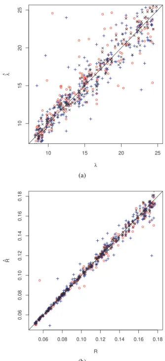
and[0.05,0.18], respectively. Simulating the modelX once for each θi = (λi,Ri), i=1, . . . ,N yielded the observations xi. The exact statistics (cAA,cLA,_cχA) and their counterparts (fAA,LfA,_fχA) for the discretizations were both applied to these observations in order to compare the performance of the estimation methods. Fig. 1 presents the true parameters plotted against their estimated values obtained from a single-run SQS and EQS estimation for each θi. The mean number of newly added locations in case of running the SQS estimation method based on the exact statistics

(Eq. 24) amounted to 20 whereas using the discretized versions required 35 additional sampling locations on average.

TheBayesian root mean square error(BRMSE)

BRMSE=

s

1 N

N

∑

(θik−θˆik)2, k=1,2

ofNre-estimated parameters was separately calculated over ˆθi= (λˆi,Rˆi)for each estimation method.

For 13 out of 200 single-runs of the SQS estimation method the current implementation caused the method to fail to converge towards the “correct” root. This algorithmic behaviour due to the current implementation of the SQS estimation method is induced by the non-convexity properties of the quasi-score in general, thus making it difficult to distinguish between multiple roots (Heyde, 1997, sect. 13.3).

First of all the BRMSE for the estimators based on the method of intensities, see Table 1, show a well-known behaviour, namely, that MIb outperforms MIa due to the fact that the estimators for the specific Euler number χA have much higher variability than that for

AA andLA (Chiuet al., 2013). For both MIa and MIb the relatively high BRMSE of ˜λ and ˜R compared to that of ˆλ and ˆRis due to the fact that the estimators f

LA andfχAbased on the discretized realizations are not

unbiased forLAandχA, respectively, see Serra (1982); Ohser and M¨ucklich (2000). This also leads to a bias for ˜λ and ˜R, which is here quite pronounced because of the very coarse applied discretization.

Table 1. Bayesian root mean square error (BRMSE) for the estimators ofλ and R according to the method of intensities with (AA,LA,χA) (MIa), with (AA,LA)

(MIb), exact score (EQS), and simulated quasi-score (SQS) estimation. Values are rounded to two significant digits. The simulation study standard errors are given in parentheses. The exact quasi-score is not applicable for the discretized data.

Method BRMSE(bλ) BRMSE(eλ)

MIa 1.8 (0.21) 9.5 (0.36) MIb 1.3 (0.10) 7.0 (0.21)

EQS 1.1 (0.07) –

SQS 2.5 (0.32) 2.5 (0.34)

Method BRMSE(Rb) BRMSE(Re)

MIa 0.011 (0.0029) 0.299 (0.0674) MIb 0.003 (0.0003) 0.044 (0.0017)

EQS 0.003 (0.0002) –

10 15 20 25

10

15

20

25

λ

λ

^

(a)

0.06 0.08 0.10 0.12 0.14 0.16 0.18

0.06

0.08

0.10

0.12

0.14

0.16

0.18

R

R

^

(b)

Fig. 1. Plot of 200 re-estimated parameters vs. true parameters for (a) λ and (b) R using the estimators(λˆSQS,RˆSQS)(red), (e_λSQS,ReSQS)(blue) and

(λˆEQS,RˆEQS)(black).

Furthermore, although the BRMSE of the new SQS estimation method using exact statistics is higher than that of MIa and MIb, the BRMSE of the EQS estimation method is smaller than that of MIb, i.e., EQS even outperforms MIb. On the one hand this demonstrates that the quasi-score estimation method can use the available statistical information in an optimal way, thus yielding more precise parameter

estimates. On the other hand it shows that the applied simulation-based implementation of the quasi-score method (SQS) cannot fully exhaust the theoretically possible potential. The reasons for the latter are that Monte Carlo simulation is involved and that in a few cases “wrong” roots are found (see the above discussion), leading to a higher BRMSE.

However, Table 1 also shows that the BRMSE of the new SQS estimation method using the exact or discretized version of the statistics are of the same order of magnitude (cf. also Fig. 1) and that for the case of discretized data SQS clearly outperforms MIa and MIb. This is because in the SQS estimation method the observed and simulation-based statistics are equally treated with respect to the way of how the data is observed, namely, in both cases the estimation of the statistics is based on the discretized model realizations. In particular it is not important whether or not the characteristics (AA,LA,χA) are estimated unbiasedly. More generally, it is even irrelevant for the SQS estimation procedure whether the used statistics possess any direct interpretation,e.g., whether they are estimators of any certain model characteristics. This is one of the fundamental strengths of the proposed SQS estimation method.

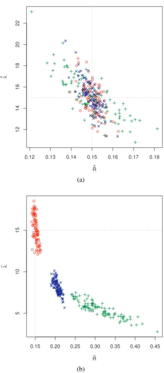
In the remainder of this section we assess the precision of the SQS estimates and compare it to the error predicted by the inverse quasi-information matrix. We generated N =100 observations of the model at the fixed parameter value θ = (15,0.15) and applied the above two kinds of statistics to these observations as we did in the first part. The SQS estimation method was applied, the resultant estimates are shown in Fig. 2 including the MIa and MIb estimates. Fig. 2a shows the comparable performance of the three estimators (MIa, MIb and SQS) in case of exact statistics. Fig. 2b shows again the problem generated by the bias of the estimators of LA and χA in case of discretized data leading to a substantial bias for the method-of-intensities estimators.

The comparison of the empirical estimation error with the predicted error is based on the empirical mean squared error matrixMSEM=_N1∑Ni=1(θ−θˆi)(θ−θˆi)t either in the case of the exact statistics, denoted as

\

MSEM, or for their discretized counterparts,MSEM^ . They read

\

MSEM=

2.03 −3.05·10−3 −3.05·10−3 1.56·10−5

,

^

MSEM=

2.68 −5.00·10−3 −5.00·10−3 2.80·10−5

.

the mean squared error matrix of ˆθ. We thus compare this to the average

Σ= 1 N

N

∑

I(θˆi)−1∈Rq×q (25)

of the approximated quasi-information matrices in the estimated parameter value for each of the 100 simulations, which read, respectively,

ˆ

Σ=

2.03 −4.27·10−3 −4.27·10−3 2.99·10−5

,

˜

Σ=

3.19 −2.86·10−3 −2.86·10−3 2.61·10−5

.

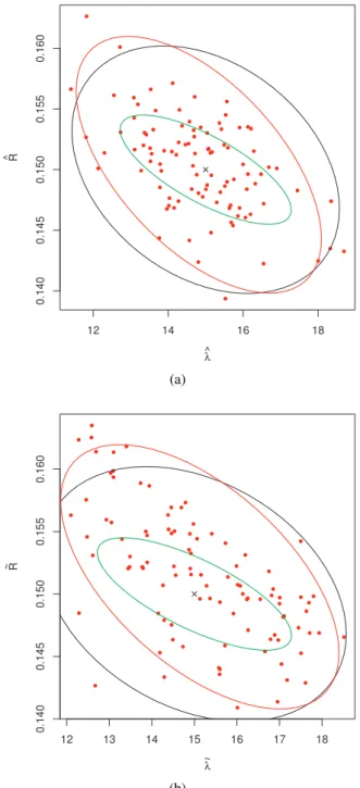
Both compare well to the corresponding observed mean squared error matrix. Fig. 3 compares them graphically. The exact quasi-score method provides a different quasi-information matrix,

I(θ)−1=

1.30 −1.89·10−3 −1.89·10−3 5.07·10−6

,

which would suggest a lower estimation error. This corresponds to the fact that this method is more precise. It can be expected that using more simulations would allow to increase the performance of the SQS method towards EQS. The theoretical and empirical evidence thus suggests that the inverse quasi-information might serve as an estimate for the precision of the method. More studies are, however, required to support generalizability of this result.

DISCUSSION

The new simulation-based quasi-likelihood method allows to estimate parameters for statistical models where neither the likelihood nor moments or characteristics can be computed directly. The user is only required to provide informative statistics and a method to simulate realizations of these statistics for different model parameters. Based on an iterative simulation procedure providing successively improved approximations to the quasi-score function, the estimation algorithm provides a numerical approximation to the efficient likelihood estimation method. The inverse of the quasi-information matrix computable on the approximation seems to provide a good measure of the estimation error. This allows estimation of model parameters in very general settings.

0.12 0.13 0.14 0.15 0.16 0.17 0.18

12

14

16

18

20

22

R^

λ

^

(a)

0.15 0.20 0.25 0.30 0.35 0.40 0.45

5

10

15

R ~

λ

~

(b)

Fig. 2. Re-estimated parameters by SQS (red), MIa (green), MIb (blue) for 100 realizations of the data at (λ,R) = (15,0.15)using the statistics (a)(cAA,cLA,_cχA)

or (b)(fAA,LfA,fχA).

can not be computed. However, if they could be computed and the statistics are well chosen, one would typically expect better or similar performance to most known estimation procedures. ML estimators

12 14 16 18

0.140

0.145

0.150

0.155

0.160

λ ^

R

^

(a)

12 13 14 15 16 17 18

0.140

0.145

0.150

0.155

0.160

λ

~

R

~

(b)

Fig. 3. Re-estimated parameters by the SQS for 100 realizations of the data at (λ,R) = (15,0.15) using the statistics (a) (AcA,LcA,χcA) or (b)(fAA,fLA,fχA). The

2σ-ellipses are given for the averaged inverse quasi-information (black), the empirical mean squared error matrix of the residuals (red), and the exact inverse quasi-information matrix of the exact quasi-likelihood-method (green). The figure illustrates the matching of the first two.

in exponential families are special cases of quasi-likelihood estimators. Quasi-quasi-likelihood estimators use moments more efficiently than typical method-of-moment estimators and can use more information.

ACKNOWLEDGMENTS

This research has been supported by the German Federal Ministry of Education and Research under grant 03MS603B/05M10OFA. We are grateful to Andr´e Tscheschel for the opportunity to use his Morph2D software.

REFERENCES

Altendorf H, Jeulin D (2011). Random-walk-based stochastic modeling of three-dimensional fiber systems. Phys Rev E 83:041804.

Ballani F (2007). The surface pair correlation function for stationary Boolean models. Adv Appl Probab SGSA 39:1–15.

Chiles JP, Delfiner P (1999). Geostatistics: Modelling spatial uncertainty. New York: J. Wiley & Sons. Chiu SN, Stoyan D, Kendall WS, Mecke J (2013).

Stochastic geometry and its applications. Chichester: J. Wiley & Sons, 3rd ed.

Cressie NAC (1993). Statistics for spatial data. New York: J. Wiley & Sons.

Gaiselmann G, Froning D, Toetzke C, Quick C, Manke I, Lehnert W,et al. (2013). Stochastic 3D modeling of non-woven materials with wet-proofing agent. Int J Hydrogen Energ 38:8448–60.

Godambe VP, Heyde CC (1987). Quasi-likelihood and optimal estimation. Int Stat Rev 55:231–44.

Golub GH, Loan CFV (1996). Matrix Computations. Baltimore, MD, USA: JHU Press.

Heinrich L (1993). Asymptotic properties of minimum contrast estimators for parameters of Boolean models. Metrika 31:349–60.

Heyde CC (1997). Quasi-likelihood and its applications: A general approach to optimal parameter estimation. New York: Springer.

Illian J, Penttinen A, Stoyan H, Stoyan D (2008). Statistical analysis and modelling of spatial point patterns. Chichester: J. Wiley & Sons.

Kleijnen JPC, van Beers WCM (2009). Kriging metamodeling in simulation: A review. Eur J Oper Res 192:707–16.

Lautensack C (2008). Fitting three-dimensional Laguerre tessellations to foam structures. J Appl Statist 35:985– 95.

functions in the presence of nuisance parameters. Statist Sci 10:158–73.

Mardia KV (1996). Kriging and splines with derivative information. Biometrika 83:207–21.

Mardia KV, Marshall RJ (1984). Maximum likelihood estimation of models for residual covariance in spatial regression. Biometrika 71:135–46.

Matheron G (1973). The intrinsic random functions and their applications. Adv Appl Probab 5:439–68. Mecke KR (2001). Exact moments of curvature measures in

the Boolean model. J Stat Phys 102:1343–81.

Molchanov IS (1997). Statistics of the Boolean model for practitioners and mathematicians. New York: J. Wiley & Sons.

Møller J, Waagepetersen RP (2003). Statistical inference and simulation for spatial point processes. Boca Raton: Chapman & Hall/CRC.

Nott DJ, Ryd´en T (1999). Pairwise likelihood methods for inference in image models. Biometrika 86:661–76. Ohser J, M¨ucklich F (2000). Statistical analysis of

microstructures in materials science. Chichester: J. Wiley & Sons.

Ohser J, Schladitz K (2009). 3D images of materials structures. Weinheim: Wiley-VCH.

Osborne MR (1992). Fisher’s method of scoring. Int Stat Rev 60:99–117.

Redenbach C (2009). Microstructure models for cellular materials. Comp Mater Sci 44:1397–407.

Sacks J, Welch WJ, Mitchel TJ, Wynn HP (1989). Design

and analysis of computer experiments. Statist Sci 4:409–23.

Santner T, Williams B, Notz W (2003). The design and analysis of computer experiments. New York: Springer. Schneider R, Weil W (2008). Stochastic and integral

geometry. Berlin: Springer.

Serra J (1982). Image analysis and mathematical morphology. London: Academic Press.

Spall JC (2003). Introduction to stochastic search and optimization: estimation, simulation, and control. Hoboken, New Jersey: J. Wiley & Sons.

Torquato S (2002). Random heterogeneous materials: microstructure and macroscopic properties.. New York: Springer.

Tscheschel A (2005). R¨aumliche Statistik zur Charakterisierung gef¨ullter Elastomere. Ph.D. thesis, TU Bergakadmie Freiberg, Germany.

Varin C (2008). On composite marginal likelihoods. Adv Statist Anal 92:1–28.

Wackernagel H (2003). Multivariate geostatistics. Berlin: Springer.

Wahba G (1990). Spline models for observational data. Philadelphia, PA: SIAM.

Wilson RJ, Nott DJ (2001). Review of recent results on excursion set models. Image Anal Stereol 20:71–8. Zimmermann DL (1989). Computationally efficient