STATISTICAL ANALYSIS OF TOMOGRAPHIC RECONSTRUCTION ALGORITHMS BY MORPHOLOGICAL IMAGE CHARACTERISTICS

STATISTICAL ANALYSIS OF TOMOGRAPHIC RECONSTRUCTION

ALGORITHMS BY MORPHOLOGICAL IMAGE CHARACTERISTICS

S

L ¨

A

K

A

L

M

P. H

V

S

1_{Institute of Stochastics, Ulm University, D-89069 Ulm, Germany;}2_{BAM Federal Institute for Materials}

Research and Testing, D-12200 Berlin, Germany e-mail: [email protected]

(Accepted March 17, 2010)

ABSTRACT

We suggest a procedure for quantitative quality control of tomographic reconstruction algorithms. Our task-oriented evaluation focuses on the correct reproduction of phase boundary length and has thus a clear implication for morphological image analysis of tomographic data. Indirectly the method monitors accurate reproduction of a variety of locally defined critical image features within tomograms such as interface positions and microstructures, debonding, cracks and pores. Tomographic errors of such local nature are neglected if only global integral characteristics such as mean squared deviation are considered for the evaluation of an algorithm. The significance of differences in reconstruction quality between algorithms is assessed using a sample of independent random scenes to be reconstructed. These are generated by a Boolean model and thus exhibit a substantial stochastic variability with respect to image morphology. It is demonstrated that phase boundaries in standard reconstructions by filtered backprojection exhibit substantial errors. In the setting of our simulations, these could be significantly reduced by the use of the innovative reconstruction algorithm DIRECTT.

Keywords: metrology, morphological image analysis, non-destructive testing, phase boundary, reconstruction algorithm, tomography.

INTRODUCTION

The principle of tomographic reconstruction of a volume from lower-dimensional projections as,

e.g., applied in X-ray or electron tomography was

mathematically discovered by Radon (1917). For a comprehensive introduction and important aspects of applications see, e.g., Frank (2005), Banhart (2007), and Buzug (2008). Tomographic reconstructions can be computed by a variety of different techniques such as filtered backprojection (FBP) (Feldkamp et al., 1984; Kak and Slaney, 1988), algebraic reconstruction techniques (ART) (Gilbert, 1972; Carazo et al., 2005), geometric tomography (Gardner, 1995) or discrete tomography (Batenburg, 2005; Herman and Kuba, 2007). The comparative evaluation of these algorithms is naturally dependent on the choice of quality criteria. These are mathematically formulated by a figure of merit (FOM) measuring the deviation of a phantom data set from its reconstruction, which is computed from simulated projections of the phantoms. Since ranking of the reconstruction quality provided by different algorithms is FOM-dependent (Herman and Odhner, 1991), FOMs need to be chosen in a task-oriented way (Hanson, 1990). That means, the FOM needs to detect differences in reconstruction quality which are relevant to the further analysis

of the tomograms in a specific application, e.g., from medicine or materials science. Typical FOMs for medical applications are based on curves of the receiver operator characteristics. They allow to study the detectability of different tissues and thus the reliability of diagnostics (Herman and Yeung, 1989; Hanson, 1990). There is a large variety of FOMs focusing on the correct reproduction of gray values. The most common representative of gray value oriented FOMs is the mean squared deviation

d=

s

∑

j

³

xrec_j −xphan_j

´2.

s

∑

j

³

xphan_j

´2

, (1)

which averages over the gray value differences xrec_{j −}

xphan_j between all pixels j in the reconstruction and the phantom (Gilbert, 1972; Hansis et al., 2008). Alternatively, mean absolute differences of gray values as well as deviations of gray value means and variances in the reconstruction from the respective values of the phantom have been considered (Sorzano et al., 2001). Moreover, phase-specific mean gray values have been used to assess the detectability of different components within a material (Sorzano et al., 2001).

be a valuable source of information for assessing the quality of a tomogram (Lange et al., 2008). These residuals are obtained by subtracting a simulated projection of the reconstruction from the measured projection for all rotation angles.

All approaches described above focus on global accuracy of the reconstruction, whereas evaluation results can hardly be interpreted with respect to the preservation of locally defined image characteristics such as little cracks in the material or the exact shape of phase boundaries. Correct reconstruction of locally defined characteristics is however crucial for unbiased computation of morphological image characteristics such as connectivity, boundary length or surface area. Quantitative information on these characteristics is a valuable source of information in a wide range of applications such as metrology (Neuschaefer-Rube

et al., 2008), pathology (Mattfeldt et al., 2007),

environmental health (Stoeger et al., 2006) or design of materials (Frost et al., 2006). We therefore suggest to directly incorporate measurements of morphological image characteristics into the FOMs used to evaluate tomographic reconstruction algorithms. Apart from measurements of phase boundary length and surface area (see, e.g., Park et al., 2000) many other morphological characteristics such as connectivity (Ohser and Schladitz, 2008) and fractal dimension (Baumann et al., 1993) are sensitive to the shape of phase boundaries. We nevertheless decided to assess local reconstruction quality along phase boundaries by measuring deviations in boundary length between the original 2D phantom images and their tomographic reconstructions. Other approaches, which have been suggested to study reconstruction quality with focus on the vicinity of phase boundaries, are based on weighted averaging of gray value deviations between phantom and reconstruction (Sorzano et al., 2001), where weighting is with respect to distance from phase boundaries. In contrast to this FOM our method provides a direct assessment of reconstruction quality in terms of quantitative morphological image analysis. Previous methods to locally evaluate reconstruction quality consider average gray value deviations within certain regions of interest (Furuie et al., 1994) and thus have the additional disadvantage that these regions need to be specified a priori.

The two principle questions arising in comparison of reconstruction algorithms ask for the relevance and for the significance of differences in reconstruction quality, respectively. Relevant differences can possibly be detected by computation of an appropriately chosen FOM for a single phantom such as the well-known section of a head introduced in Shepp and Logan (1974). The use of such deterministic input offers

even to a specific experimental instrument need to be taken into account. Simulations of projections would thus, e.g., incorporate noise, beam hardening, limited rotation or alignment problems (Carazo et al., 2005; Haibel 2008).

In the following the suggested methodology will be applied to investigate the performance of standard FBP algorithms in comparison to the innovative reconstruction technique DIRECTT (Direct Iterative Reconstruction of Computed Tomography Trajectories) (Lange et al., 2008). The phantom data will be two-dimensional. In many applications such as electron tomography, projections are acquired in parallel beam geometry. As a consequence, tomograms of 3D volumes are a stack of 2D reconstructions from 1D projection data. Thus, in parallel beam geometry our results on 2D datasets are also relevant for the 3D case. The exact consequences for 3D morphological image analysis remain an interesting subject for future applications of our methodology.

We will see that the applied FBP algorithms alter the structure of phase boundaries in such a way that boundary length measurements are substantially affected whereas the DIRECTT reconstructions preserve boundary structures in a much better way. In a first step we will demonstrate these effects for projections of phantoms without noise (referred to as ‘ideal projections’ below). Afterwards we will show that the superiority of the DIRECTT reconstruction remains valid under the addition of simulated noise to the projection data.

The paper is organized as follows. After discussing phantom generation and simulation of projections we give an introduction to the investigated reconstruction techniques in order to illustrate their principle ideas to a non-expert reader. Then we briefly discuss the estimation techniques for measuring boundary length, leaving additional details for the appendix. Furthermore, we introduce the FOMs serving as basis for the evaluation and the statistical tests we applied. We conclude by the presentation of the results and their discussion.

METHODS

PHANTOM DATA

The phantoms projected and reconstructed for this study were discretized versions of realizations of Boolean models in 2D, which were sampled on an observation window W= [0,500]2_{(Fig.1(a)). Boolean} models are a class of random closed sets whose construction is based on a homogeneous Poisson point

pattern _{Sn}n≥1. In our specific setting we used a Boolean model which is defined as the union B = S∞

n=1B(Sn,r) of circles B(Sn,r) of radius r = 10 centered at Sn. The intensity of the homogeneous Poisson process on IR2 determining the random locations _{S_n}n≥1 was chosen such that the mean number of points in W = [0,500]2 _{was 1200. Since} reconstructions are pixel images, throughout our study we investigated discretized realizations of this Boolean model on a grid of 500_×500 pixels. The gray value of each pixel was chosen proportional to its area fraction covered by the realization of the Boolean model. Notice that gray values are chosen independently of the number of circles covering a location. All gray values were rounded to integers and the maximum gray value was set to 255. In order to allow for statistical analysis, 100 independent realizations b1, . . . ,b100 of

B were generated and discretized.

SIMULATION OF IDEAL AND NOISY PROJECTIONS

Projections were performed in parallel beam geometry. The sample was rotated in steps of 0.5◦ up to a maximum angle of 180◦. For the ideal projections model elements were projected individually and added to the sinogram, i.e., we performed a projection of mass (or density, resp.) instead of intensities. This approach is equivalent to integration over strips of detector width, and thus reflects that detector elements as well as the pixels of the phantom are not points but area elements. The detector elements had exactly the same size as the reconstruction pixels. The original observation window was extended by a two pixel edge of zero entries on all sides. The rotation axis was set at the windows’ center. In order to ensure complete visibility of the reconstruction pixels under all projection angles, the length of the line detector was chosen sufficiently large.

In order to assess the impact of noise on the reconstruction results we simulated intensity sinograms under a noisy X-ray source. Other experimental artifacts such as cross-talking, focal smearing, beam hardening or limited dynamic range (non-linearities in detection) were not simulated. For the noisy intensity measured at detector location ξ under rotation angle γ one obtains the approximative formula

Iγ(ξ) =X_ξ,γexp(−pγ(ξ)), (2)

where the process _{X_ξ,γ} denotes Gaussian white noise with fixed expectation EX_ξ,γ = µ > 0 and variance VarX_ξ,γ = σ2 _{> 0 and p}

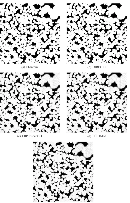
(a) Phantom (b) DIRECTT

(c) FBP Inspect3D (d) FBP IMod

(e) fast FBP

Fig. 1. Sample phantom and its reconstructions from projection data. The right upper corner has been scaled by

number of X-ray quanta with high expectation (Buzug, 2008). Notice that for each detector location ξ and rotation angle γ the recorded intensity Iγ(ξ)

has a normal distribution. However, expectation and variance differ from the respective values of the initial intensity X_ξ,γ and are given by µexp(₋p_γ(ξ)) and σ2_exp(−p

γ(ξ))2, respectively. Thus, the stochastic counting rate at the detector depends not only on the input intensity but also on the projected object. The noise level is expressed by the signal-to-noise-ratio (SNR) _σµ. In an experimental setting under Gaussian approximation of Poisson noise one has σ = √µ. However, for simulation purposes we fixed µ and variedσ, since the parameter of interest was the SNR rather than the absolute value of the initial intensity.

TOMOGRAPHIC RECONSTRUCTION ALGORITHMS

Filtered backprojection

A standard technique for the tomographic reconstruction of projection data is filtered backprojection (FBP) (Feldkamp et al., 1984; Kak and Slaney, 1988). FBP is widely utilized in computed tomography using X-rays (Buzug, 2008) as well as electrons (Carazo et al., 2005). In the following we will briefly summarize the mathematical foundations of FBP.

Let f : IR2_→[0,∞)denote a density distribution on IR2with bounded support which is to be reconstructed from the set of projections_{pγ : γ_∈[0,2π)_}whereγ denotes the rotation angle. A single projection pγ(ξ) = R

e⊥_ξ,γ f(x)dx is an integral taken along the line

e⊥_ξ,γ ={ξ

µ

cos(γ)

sin(γ) ¶

+s µ

−sin(γ)

cos(γ) ¶

: s_∈IR_}, (3)

which is perpendicular to the first axis rotated by γ and has distanceξ from the origin. The mathematical key ingredient of FBP is the Fourier slice theorem. For the Fourier transform Pγ(q) =R∞

−∞pγ(ξ)e−2πiqξdξ of

a projection pγ(ξ)at a fixed rotation angleγ_∈[0,2π)

the Fourier slice theorem states the identity (cf. Buzug, 2008)

P_γ(q) =F(q cos(γ),q sin(γ)). (4)

That is, the Fourier transform of the one-dimensional projection at rotation angleγcorresponds to the slice of the two-dimensional Fourier transformed object F passing through the origin in direction γ. Substituting polar coordinates in the formula of the inverse Fourier transform and a subsequent application

of the Fourier slice theorem yields the identity (for details cf. Buzug, 2008)

f(x) =

Z π

0 Z ∞

−∞|q|Pγ(q)e

2πqi(x1cos(γ)+x2sin(γ))dq dγ_,

for all x_∈IR2. (5)

The most commonly used FBP algorithm is based on this formula and organized as follows. In a first step the Fourier transforms P_γ(q) of the projections are computed. These are subjected to an inverse Fourier transform after radial weighting by the factor _|q_|, which yields filtered projection images. Backprojections without weighting result in a convolution of the image to be reconstructed with the point spread function 1/_kx_k (Buzug, 2008). In practice, the transforms are naturally done by discrete (inverse) Fourier transforms of the discretely sampled signal. In the backprojection step, for every pixel of the discrete output image the corresponding position on each filtered projection image is determined and the corresponding value is added to the sum which discretizes the outer integral in Eq. 5. Since this position will in most cases be a non-integer pixel position, interpolation schemes need to be applied to neighboring pixels. By Shannon’s sampling theorem, at a given real space sampling distance ∆ξ the signal can only be correctly reconstructed up to a frequency Q= (2∆ξ)−1 _{in Fourier space. Thus, the} radial weighting by the function _|q_| in Eq. 5 is only reasonable for _|q_| < Q. In other words, the

sampling scheme imposes a band limitation which naturally determines the range of integration in the discrete approximation of the inner integral in Eq. 5. In applications high frequencies are often considered as noise. Therefore, in practice frequencies are not weighted radially but the filter function is replaced by a modified version _|q_|W(q), where W(q) is a window function that decreases the weight of the high frequency band. Apart from a simple cutoff at frequency qmax (i.e., setting W(q) = 1I[0,qmax](|q|))

approach. The latter will be referred to as ‘fast FBP’. For this study the implementation of the fast FBP provided by the IMod software (Kremer et al., 1996) was applied. Notice that the license for this component is not included in the standard version. In order to assess the influence of specific implementations on the reconstruction quality of the commonly used real space FBP we computed real space FBPs by two different software packages namely Inspect3D (version 3.0, FEI companyTM_{) and the IMod software}

(version 3.11.2).

An unmodified radial filter with simple cutoff was used for comparison of FBP to other reconstruction techniques. The cutoff frequency was set to the maximum spatial frequency that could occur in our image data. We will nevertheless demonstrate the effect on reconstructions which is caused by switching to a Gaussian decay of the filter function at varying cutoff frequencies.

Both software packages we applied are designed to reconstruct 3D volumes from 2D projections. However, the software backprojects each 2D slice of the volume separately and thus each sample of our 2D phantom data could be considered as a single slice of a 3D volume. Sample reconstructions can be found in Fig.1.

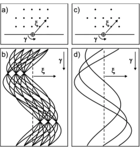
DIRECTT

The algorithm DIRECTT (Lange et al., 2008) represents a promising alternative to conventional reconstruction algorithms such as FBP or ART. Fig.2 schematically displays the algorithm’s iterative philosophy. The 2D algorithm is applicable to parallel as well as fan beam geometry of projection. In the following we study parallel beam projections as illustrated in Fig. 2, which are computed in strips for each detector element. Fig. 2a (top left) indicates a model volume at the example of a 14 pixel object. Fig.2b (bottom left) represents the respective density sinogram (Radon transform (Radon, 1917)) which is either achieved by computed projection of model densities (Fig. 2a) or is the initial experimental intensity data converted according to Lambert-Beer’s law (cf. Buzug, 2008). Demanding that each element of the reconstruction array corresponds to exactly one sinusoidal trajectory of the sinogram (Fig. 2b), the DIRECTT algorithm selects pixels, i.e., area elements, corresponding to trajectories of dominant weight for an update of the reconstruction. The given density sinogram can optionally be filtered along the detector direction. This is helpful to avoid artifact formation equivalent to the effects of an unfiltered backprojection. However, an intriguing feature of DIRECTT is that adaptations of the filter function can

be used to evaluate trajectories with focus on specific aspects of interest such as mass or contrast. Switching filters between subsequent iteration steps can be used to incorporate a variety of different aspects of the image into the reconstructions step by step. Let the discrete sinogram be given by the matrix S= (si j), such that i = 1, . . . ,N and j = ₋ℓ, . . . , ℓ, where N denotes the number of projection angles and 2ℓ+1 is the number of detector elements. Then the filtered sinogram is given by the matrix S∗, where the ith row

s∗_i of S∗is obtained by a convolution of the ith row siof

S (extended byℓzeros at both ends) with the discrete

filter function c :_{−2ℓ, . . . ,2ℓ_{} →}IR, more precisely

s∗_{i j}=∑ℓ_k=−ℓsikc(k−j).

Computation of the DIRECTT reconstructions in the present study involved switching between two different filter functions. The first six iteration steps were performed after application of the mass filter

cm(k) =

(

−1

k2 for k∈ {−2ℓ, . . . ,2ℓ} \ {0},

2∑2_˜k=ℓ_1˜k1₂ for k=0.

The subsequent steps of iteration (fourteen for reconstructions of ideal projections) were based on contrast-filtered sinograms, where the contrast filter cc is given by

cc(k) =







−1 for k_{∈ {−}1,1_},

2 for k=0,

0 else.

The weights of all possible trajectories (corresponding to integer reconstruction positions) are computed by averaging along the respective traces within the optionally filtered sinogram. This involves interpolation between neighboring sinogram pixels corresponding to different detector elements. This is a substantial difference to FBP, where interpolation is performed in Fourier space (fast FBP) or in the backprojection step after the sinogram has been (inversely) Fourier transformed and filtered (real space FBP).

inverse Radon transform. In contrast to FBP there is no integral computation along the line detector (including limited sampling due to its element size) but an optional over-sampling along the numerous projection angles. One of DIRECTT’s unique characteristics is its very precise projection of reconstruction elements taking into account their actual size and shape which is essential for enhanced spatial resolution. That is, reconstruction pixels are considered as a set of densely packed elements instead of being (circularly smeared) point functions only. Hence, all previously described calculations are performed based on squared area elements in a Cartesian matrix. DIRECTT is of particular interest when the focus is on reconstruction of finely structured details or on precise location of reconstructed elements rather than on computing time. In contrast to FBP, DIRECTT does not treat each (detector) projection individually, i.e., it is not deconvolved globally or (Fourier) filtered, but the entire trajectory of a reconstruction element is considered over all projections. In contrast to ART, DIRECTT does not modify the entity of all reconstruction elements simultaneously.

Fig. 2. Reconstruction principle of the iterative

procedure applied by DIRECTT. (a) Model volume of a 14 pixel object. (b) Density sinogram of the model. Each trajectory corresponds to one of the pixels. (c) Intermediate reconstruction array, where 11 out of the 14 pixels have been added. (d) Residual sinogram after subtraction of the sinogram generated by the intermediate reconstruction in (c) from the sinogram in (b).

ESTIMATION OF AREA AND BOUNDARY LENGTH

For the evaluation of reconstruction algorithms we compared the area as well as the boundary length as measured by two different computational methods in the discretized input data to values found

for the various reconstructed images. Notice that we are interested in the boundary length and area of the discretized version of the entire Boolean model B=S∞

n=1B(Sn,r) rather than in the cumulated morphological characteristics of the single circles

B(Sn,r), n≥1. Comparison of morphological image characteristics requires a binarization of the images, which was done by simple thresholding, where the threshold parameter was set to 50% of the maximum greyvalue. In order to exclude bias by pure scaling differences, thresholding was done after normalizing the gray values of each image in such a way that the average gray values occurring in the background and the foreground phase were set to 0 and 255, respectively.

Any attempt to measure morphological characteristics of a discretized set faces the problem that the shape of the set before discretization cannot be reconstructed from the pixel image. In order to estimate the foreground area we applied the natural approach of counting the number of foreground pixels. For estimating the original boundary length, different formulae from integral geometry and stereology can be exploited. Nevertheless, estimation results and consequently approximation errors are more than likely to differ with respect to the estimation method chosen. In order to ensure reliability of our statistical results on reconstruction quality, we therefore implemented two different methods for measuring the boundary length of the foreground phase.

The first method we applied has been introduced in Klenk et al. (2006) and further discussed in Guderlei et

al. (2007). It will be referred to as the Steiner method

since it is based on a discretized version of a Steiner-type formula known from the geometry of polyconvex sets. Details of this method are given in the appendix. As input parameter the algorithm needs a sequence of so-called dilation radii r1. . . ,rn. Measurement results are dependent on the choice of r1. . . ,rn. Therefore, for our investigations we used two different sets of dilation radii. The first choice ri = 4.2+1.3i, i =

1, . . . ,1000, was suggested in Guderlei et al. (2007),

whereas the second choice ri = 0.4+0.09i, i =

1, . . . ,158, was optimized to obtain results whose mean

coincides with the theoretical mean boundary length of the Boolean model used for phantom generation. The corresponding mean value formulae of Boolean models can be found in Schneider and Weil (2008).

by a discrete analog of Cauchy’s surface area formula, which expresses the boundary length L(K)of the set K as an integral of the total projection length of K over all directions (see appendix). The algorithms discussed in this section were implemented in the Geostoch software library (Mayer et al., 2004).

STATISTICAL TESTS FOR

COMPARISON OF RECONSTRUCTION ERRORS

Reconstruction algorithms were statistically compared via the empirical probability distribution of the reconstruction error. The error was defined as relative deviation of the morphological characteristics on the reconstructions from the phantom data. The morphological characteristics measured were boundary length and area of the foreground. The following definition of reconstruction error is given for the example of a measurement method for the boundary length which leads to an estimator ˆL for this morphological characteristic. Effects of different reconstruction algorithms on area measurements were compared in an analogous way.

Given two reconstruction algorithms A1 and A2 and an estimator ˆL for the boundary length, for the phantoms b₁phan, . . . ,b₁₀₀phan and their reconstructions

bAk

1 , . . . ,b

Ak

100, k=1,2, the relative reconstruction errors

eA1

i =

¯ ¯ ¯ ¯

ˆL(b_iphan)−ˆL(bA1_i )

ˆL(b_iphan)

¯ ¯ ¯ ¯

and

eA2

i =

¯ ¯ ¯ ¯

ˆL(b_iphan₊₅₀)−ˆL(bA2_i+50)

ˆL(b_iphan₊₅₀)

¯ ¯ ¯ ¯

(6)

were computed for i = 1, . . . ,50. Since the phantoms b₁phan, . . . ,b₁₀₀phan were discretized versions of independently sampled realizations of a Boolean model, the entire collection of errors from the two samples eA1

1 , . . . ,e

A1 50,e

A2

1 , . . . ,e

A2

50 inherited stochastic independence. Consequently, two-sample-goodness-of-fit tests could be applied in order to compare the two distributions the error samples eA1

1 , . . . ,e

A1 50 and eA2

1 , . . . ,e

A2

50 were drawn from. Given a pair of reconstruction algorithms A1 and A2, Kolmogorov-Smirnov (KST), Wilcoxon rank (WRT) and Ansari-Bradley (ABT) tests were performed. For KST and WRT two different null hypotheses were considered, firstly that the cumulative distribution functions (CDF)

FA1 and FA2 of the error distributions are equal, and

secondly, that the error of algorithm A1 tends to be smaller than the one produced by A2 in the stochastic sense defined below.

– The Kolmogorov-Smirnov test checks the null hypothesis H0 : FA1(x) = FA2(x) for all x ∈ IR

against the two-sided-alternative that the values of the two CDFs differ for some x _∈ IR. Any differences between the two samples will lead to the rejection of H0 if they are too large in the statistical sense. In the one-sided version of the KST the null hypothesis H0 : FA1(x) ≥

FA2(x)for all x∈IR is tested, which would imply

that the first sample of A1 statistically consists of

smaller values than the second one. For details

see Conover (1971, p. 309) and Gibbons (1985, p. 127).

– The Wilcoxon rank test is equivalent to the Mann-Whitney U-test. It is especially sensitive to deviations in the location parameters of FA₁ and

FA2, i.e., it is used to determine whether one of

the distribution functions is shifted relative to the other. If the random variables X1and X2have CDFs

FA1 and FA2, respectively, the two-sided version of

the WRT tests H0 : P(X1>X2) = 1₂ against H1:

P(X1>X2)6= 1₂. Thus, differences in variabilities of reconstruction errors within the two samples will not lead to the rejection of H0 as easily as differences in the means or medians of the two samples. The one-sided version tests H0: P(X1<

X2)≥1₂against H1: P(X1<X2)<1₂, i.e., whether the sample of A1 is statistically smaller than the second sample. For mathematical details, see, e.g., Gibbons (1985, p. 164) and Lehmann and Romano (2005, p. 243).

– The Ansari-Bradley test assumes that FA1(x−m) =

FA2(θ(x−m))for all x∈IR, an unknown nuisance

parameter m used to normalize the location of the sample and some scaling ratio θ > 0. The test focuses on the question if the distributions differ in dispersion rather than in location. Thus, the ABT tests H0 :θ =1 against H1 :θ 6=1. One-sided alternatives are possible but not considered in this study. Details can be found in Gibbons (1985, p. 179).

For all tests in this study version 2.8.1 of the R programming language (R Development Core Team, 2007) was applied. Test results are given in terms of a p-value, which is the largest level of significance at which the null hypothesis is not rejected.

RESULTS

centered vertical lines show the smallest and largest observations if their distance from the box does not exceed 1.5 times the box size. More extreme values within the sample are plotted as circles. Note that in the boxplots we consider signed relative errors, where these quantities are defined as in Eq. 6 but without taking absolute values. However, all statistical tests are based on unsigned relative errors.

RECONSTRUCTIONS FROM IDEAL PROJECTIONS

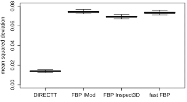
For DIRECTT the classic FOM of MSD defined in Eq.1had a value of 0.0139, whereas the corresponding values for the FBP algorithms were in the interval between 0.069 and 0.074, with best results for the Inspect3D software and the highest error measured for the standard FBP in IMOD (Fig. 3). Although very small, the differences in MSD between the FBP techniques were found to be statistically significant by KST and WRT. This is plausible since there was hardly stochastic variability in the single MSD samples.

DIRECTT FBP IMod FBP Inspect3D fast FBP

0.00

0.02

0.04

0.06

0.08

mean squared deviation

Fig. 3. Mean squared deviations of reconstructions

from original phantoms.

The area measurements of the foreground phase behaved rather stable under all reconstruction algorithms and relative errors were only at the level of few per mille (Fig. 4). Errors fluctuated around 0 for DIRECTT and were only around 0.002 for the fast FBP and the Inspect3D software. The standard FBP implemented in IMod showed a slightly increased error level of around 0.006. KST and WRT classified the differences between the algorithms as statistically significant, though the absolute level was very small.

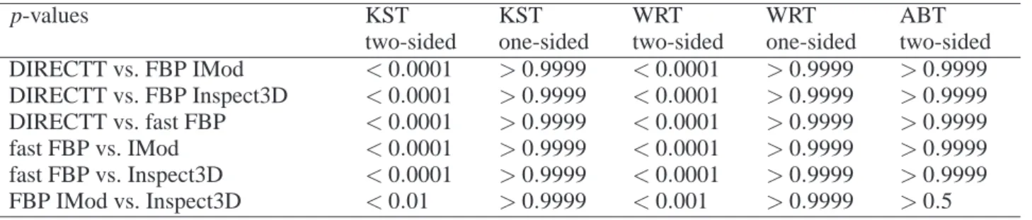
Boxplots in Fig. 5 indicate that the signed relative errors for measurements of boundary length differed between reconstruction algorithms. Stochastic variability of the errors within the sample was similar for all four reconstruction algorithms as indicated by the high p-values of the Ansari-Bradley test (Table1). In the DIRECTT reconstructions the Steiner

method measured a decrease in boundary length of around 1.5% and the Cauchy method a decrease of around 0.5% in comparison to the original phantoms. However, the FBP algorithms produced significantly higher relative errors than DIRECTT as indicated by the p-values of the tests in their one-sided versions in Table1. The error produced by the fast FBP algorithm was significantly smaller than the error produced by the standard FBP implemented in IMod, which in turn was slightly but significantly smaller than the error found in the FBP reconstruction done with Inspect3D.

DIRECTT FBP IMod FBP Inspect3D fast FBP

−0.002

0.002

0.006

0.010

signed relative error

Fig. 4. Relative deviation of area measurements on

reconstructions from original phantoms.

For all reconstruction algorithms error levels depended on the method used to measure boundary length. Averaging over all three FBP implementations, the Steiner method yielded a slightly stronger decrease in boundary lengths of around 13%. The choice of radii for the Steiner method had only a hardly noticeable impact on the measurements of relative errors (Fig. 5a vs. Fig. 5b). In summary, it should be emphasized that on the FBP-reconstructions all methods of measurement consistently indicated a decrease of boundary length in comparison to the original phantoms, whereas the deviation on the DIRECTT reconstructions was significantly smaller. All p-values of tests for equality of error distributions were so small that the KST as well as the WRT detected differences when the level of significance was set toα=0.001/2. This in particular implies that the hypothesis of equal error distributions was rejected in a Bonferroni-corrected setting for multiple testing at level α =0.01. The latter defines that a hypothesis

H0 is rejected at a level α once a single one of n tests performed on the same data rejects H0 at level

α/n. As a consequence, the probability of a false

a conservative estimate for the type 1 error of the test.

DIRECTT FBP IMod FBP Inspect3D fast FBP

−0.20

−0.15

−0.10

−0.05

0.00

0.05

signed relative error

(a) Steiner method; dilation radii ri=4.2+1.3i, i=1, . . . ,1000

DIRECTT FBP IMod FBP Inspect3D fast FBP

−0.20

−0.15

−0.10

−0.05

0.00

0.05

signed relative error

(b) Steiner method; dilation radii ri=0.4+0.09i, i=1, . . . ,158

DIRECTT FBP IMod FBP Inspect3D fast FBP

−0.20

−0.15

−0.10

−0.05

0.00

0.05

signed relative error

(c) Cauchy method

Fig. 5. Relative deviation of boundary length

measurements on reconstructions from original

phantoms.

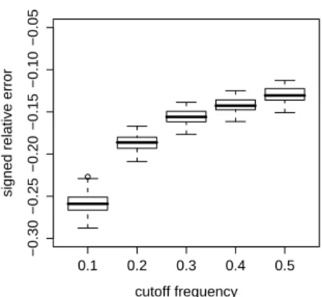
The cutoff frequency, at which FBP algorithms switch from highpass to Gaussian filtering of the Fourier transformed projections before backprojecting them, had a noticeable impact on the error in boundary length measurement. Suppression of high frequencies increased the relative deviation in boundary length measurements on the reconstructions from the original images independently of the method of measurement

(Fig.6).

0.1 0.2 0.3 0.4 0.5

−0.30

−0.25

−0.20

−0.15

−0.10

−0.05

cutoff frequency

signed relative error

(a) Steiner method; dilation radii ri=4.2+

1.3i, i=1, . . . ,1000

0.1 0.2 0.3 0.4 0.5

−0.30

−0.25

−0.20

−0.15

−0.10

−0.05

cutoff frequency

signed relative error

(b) Cauchy method

Fig. 6. Relative deviation of boundary length

measurements on FBP reconstructions from original phantoms for different cutoff frequencies. These reconstructions were performed by the real space FBP algorithm implemented in the IMod software. The highest spatial frequency that could occur in the image

data was 0.5.

RECONSTRUCTIONS FROM NOISY PROJECTIONS

projections as described in Section “Simulation of ideal and noisy projections”. These were then used as input data for DIRECTT and FBP.

SNR

relative error

−0.2

−0.15

−0.1

−0.05

0

0.05

50 100 150 200 250 300 350 400

(a) Steiner method; dilation radii ri=4.2+

1.3i, i=1, . . . ,1000

SNR

relative error

−0.2

−0.15

−0.1

−0.05

0

0.05

50 100 150 200 250 300 350 400

(b) Cauchy method

Fig. 7. Sensitivity of relative errors of boundary length

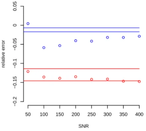
measurements to noise in the projections. The red lines mark a 96% confidence interval of the error under ideal, i.e., noiseless projections found for FBP, the blue lines mark a corresponding confidence interval for DIRECTT. Red points are reconstruction errors of FBP found for single randomly picked phantoms under the noise level depicted on the x-axis. The blue points are the corresponding errors using DIRECTT.

For noisy projections the quality of the DIRECTT reconstructions improved in terms of MSD over the first iterations but from a certain point on decreased again. This deterioration of the reconstruction quality occurs when the residual sinograms are dominated by noise and thus, further iterations introduce erroneous information into the reconstructions. The number of iterations for the DIRECTT reconstructions under noise evaluated in Fig. 7 was chosen such that MSD was minimized. Fig. 7 shows that the error of

the DIRECTT reconstructions under noise was not contained in the confidence interval of the error under ideal projections. For SNRs higher than 150 the FBP reconstructions from noisy input data stayed within or close to the range of error under ideal projections. Nevertheless, the relative loss in boundary length caused by DIRECTT was in all cases less than in the FBP reconstructions. SNRs of less than 20 did not yield reasonable reconstruction results.

DISCUSSION

Our results demonstrate that standard FBP reconstruction algorithms for projection data may alter the boundary structure of two-phase phantom images in such a way that measurements of boundary length are substantially affected. As a standard gray value oriented global measure of reconstruction quality, MSD already indicated errors in the FBP reconstructions. Locally defined image characteristics such as phase boundaries and quantitative image characteristics can however hardly be related to global integral FOMs such as MSD in a direct way. Thus, for monitoring reconstruction artifacts distorting fine details and their consequences for quantitative image analysis it is important to consider alternative FOMs. In this context boundary length measurements can be a valuable source of information since they are sensitive to changes of local pixel configurations. Corresponding FOMs can thus provide a more comprehensive view on reconstruction quality.

Apart from boundary length also other characteristics frequently considered in quantitative morphological image analysis and spatial statistics such as connectivity (Ohser and Schladitz, 2008; Thiedmann et al., 2009), spherical contact distribution function (Mayer, 2004; Thiedmann et al., 2008) and fractal dimension are dependent on adequate reproduction of phase boundaries. Since we have seen that FBP algorithms alter the structure of phase boundaries, estimation of these image characteristics from FBP reconstructions occurs to be problematic, even if comparative studies of different materials or scenarios may still be possible. On the other hand, foreground area showed very limited sensitivity to the reconstruction artifacts produced by FBP algorithms. Thus, measurements of foreground area can be regarded as stable with respect to standard FBP techniques.

Table 1. Bounds for the p-values of the tests conducted for comparison of the relative errors of boundary length

produced by the different reconstruction algorithms under noiseless projections. Small p-values of two-sided WR and KS tests indicate that error distributions are significantly different. Large p-values of the one-sided KST and WRT mean that the first of the algorithms in column 1 produces a significantly smaller error than the other one. Large p-values of the two-sided ABT suggest that the variability of the errors is similar for the two reconstruction algorithms considered.

p-values KST KST WRT WRT ABT

two-sided one-sided two-sided one-sided two-sided DIRECTT vs. FBP IMod <0.0001 >0.9999 <0.0001 >0.9999 >0.9999 DIRECTT vs. FBP Inspect3D <0.0001 >0.9999 <0.0001 >0.9999 >0.9999 DIRECTT vs. fast FBP <0.0001 >0.9999 <0.0001 >0.9999 >0.9999 fast FBP vs. IMod <0.0001 >0.9999 <0.0001 >0.9999 >0.9999 fast FBP vs. Inspect3D <0.0001 >0.9999 <0.0001 >0.9999 >0.9999 FBP IMod vs. Inspect3D <0.01 >0.9999 <0.001 >0.9999 >0.5

to compare the errors of different algorithms. Since differences between error distributions of boundary length measurements for the considered reconstruction algorithms were rather pronounced (see the boxplots in Fig.5) the unambiguous p-values of the Kolmogorov-Smirnov and the Wilcoxon rank test in Table 1 were to be expected. The Ansari-Bradley test indicated that dispersion of the error samples was not significantly different between algorithms and was probably mainly controlled by the stochastic variability of the phantom data.

The testing methodology we suggested can be transferred to any other FOM and set of randomly sampled phantom data. This way also subtle differences in reconstruction quality can be evaluated with statistical rigor. It should again be emphasized that a statistical approach to the evaluation of reconstruction quality essentially relies on randomly sampled phantoms. Reconstruction of deterministic phantom data is a valuable tool to investigate the capability of reconstruction algorithms to reproduce certain predefined image features. An approach based on randomly sampled phantoms is complementary since it can be used to monitor the statistical significance of errors produced by reconstruction algorithms. This information is especially important for the quantitative investigation of irregularly structured materials.

Throughout this study the relative error in boundary length was measured by two different techniques and – for the Steiner method – two choices of parameters. This way bias introduced by boundary measurement techniques could be excluded. Since the methods are based on discrete approximations of different formulae for the boundary length of a polyconvex set (see Appendix), deviations in

measurement results naturally occurred. Although relative errors measured by the Cauchy method were found to be slightly smaller than the errors measured by the Steiner method, qualitative as well as statistical findings agreed for all methods applied. Thus, our findings were not tied to a specific measurement approach.

In order to relate the errors caused by the general technique of FBP to the effect caused by different algorithmic approaches, FBP reconstructions were conducted by the standard real space FBP and the fast FBP algorithm suggested by Sandberg et

al., 2003. Moreover, for the real space FBP two

in real space FBP algorithms are the interpolation schemes applied in the backprojection step. Both real space FBP implementations used a computationally fast linear interpolation. The slight superiority of the fast FBP is possibly the result of the Fourier space approach, which may reduce interpolation errors along boundaries.

Cutoff frequencies applied in FBPs can hamper correct reconstructions of phase boundaries in a substantial way (Fig.6). This effect is plausible since edges are represented by high frequencies in Fourier space. It can also be expected to occur for other types of window functions which reduce the impact of high frequencies in comparison to simple radial weighting.

For ideal projection data DIRECTT presented itself as a powerful reconstruction algorithm, which reproduced phase boundaries in an almost perfect way. This has been achieved under the simple but essential assumptions of homogeneous density within the pixels, regarded as area elements, and identical pixel sizes within the model, the detector and the reconstruction. First tests with DIRECTT however indicated that the reconstruction quality is still remarkable when pixels of smaller size than the detector elements are reconstructed (Lange and Hentschel, 2007).

In order to challenge the results obtained for noiseless projections, noise of different level was added to the projection data of single randomly chosen phantoms and the reconstruction results of DIRECTT and FBP were compared. The FBP reconstructions exhibited a high noise tolerance, since the relative error in boundary length measurement did hardly leave an empirical 96% confidence interval that had been computed for the ideal projections (Fig.7). This shows that under noisy projections the reconstruction error in the phase boundaries is not dominated by the noise but by properties of the FBP technique. The DIRECTT reconstructions reacted more sensitively to the noise, since the errors increased and were outside the 96% confidence interval for the DIRECTT reconstructions under ideal projections. Nevertheless, in all cases the DIRECTT reconstructions exhibited a substantially smaller error than the FBP tomograms. Thus, the improvement in reconstruction quality that can be achieved by DIRECTT appears to not to be limited to ideal sets of input data but can also be expected in experimental settings. The simulated projections of pixel data serving as input for the reconstruction algorithms do not exactly describe a tomographic experiment with a spatially continuous material. However, our methods chosen for the transformation of the spatially continuous realizations of the Boolean model into pixel phantoms and the computation of

the projections by strip integrals yield an adequate approximation of an experimental setting.

It should be mentioned that it is difficult to determine the optimal number of iterations for the reconstruction of noisy experimental input data. It is a challenging problem to judge whether a residual sinogram is dominated by erroneous information from projection noise and hence, further steps of iteration will only result in artifacts. This is an important subject for further studies.

The merits of the DIRECTT reconstructions come at the cost of increased computation time, which totaled 22 min on an Intel Xeon 5130 processor (2.0 GHz, one core) for a single input image. However, standard algebraic reconstruction algorithms such as SIRT (Gilbert, 1972), which is commonly used in electron tomography (Bals et al., 2007), are also computationally more demanding than FBP. In contrast to DIRECTT, in addition to the number of iterations, they usually require optimization of other parameters in order to yield satisfactory results (Carazo et al., 2005). Since for our phantom data a SIRT reconstruction computed by the Inspect3D software with 20 iterations exhibited substantially increased blurring at the phase boundaries in comparison to the FBP results, we did not include SIRT in our comparative analysis.

It is possible that other backprojection techniques than standard FBP are capable of an improved representation of phase boundaries. These algorithms comprise λ-tomography, where local inversion formulae ensure that space-continuously defined functions and their theoretical reconstructions have the same jumps. One should however point out that λ-tomography does not reconstruct the density distribution f itself but the function Λf , where

Λ=√_−△denotes the Calderon operator which does not preserve gray values (for details see Louis and Maass, 1993; Kuchment et al., 1995; Faridani et al., 1997). An innovative and computationally efficient reconstruction technique has been proposed by Louis (2008). This approach combines reconstruction and edge detection and could also enable superior reconstructions of phase boundaries in comparison to standard FBP techniques. Furthermore, for samples consisting of few different materials such as our phantom data, algorithms from discrete tomography have been reported to be very promising tools for tomographic reconstruction (Batenburg, 2005; Bals

et al., 2007; Herman and Kuba, 2007). Discrete

caused by limited rotation of the sample (Lange

et al., 2008). Furthermore, they return an image

which does not require segmentation of the different materials. By construction, DIRECTT also offers the option to compute discrete tomograms and thereby to reconstruct details which cannot be extracted from the projections in the standard setting. Nevertheless, our results demonstrate that even without the a priori information needed for discrete tomography mode, DIRECTT reconstructions exhibit a level of contrast and detail preservation which is not achieved by conventional FBP reconstruction.

We have illustrated that under ideal and noisy projections reconstruction algorithms can cause statistically significant changes of image morphology. For practical applications the error caused by the reconstruction algorithms needs to be carefully related to the effect of experimental imperfections in the projection data. These may comprise alignment deviations, the specific noise level or limited rotation. Expert knowledge about these experimental conditions is important to identify appropriate reconstruction algorithms and their parameters, that meet the specific needs of an application. Nevertheless, whenever realistic projections can be simulated and a FOM capturing the aspects of interest has been defined, randomly generated phantom data reflecting the structural properties of the investigated object and statistical analysis provide a powerful setting to compare different reconstruction techniques.

APPENDIX

MEASURING BOUNDARY LENGTH BY THE STEINER METHOD

The algorithm for boundary length measurement we refer to as the Steiner method exploits the following Steiner-type formula: Let K _⊂IR2 be polyconvex set,

i.e., a finite union of convex sets, then for r>0 the

so-called weighted volumeρr(K) of the set K can be written as

ρr(K) =r2πV0(K) +rV1(K), (7)

where 2V1(K) is the boundary length L(K) of K and

V0(K) denotes the Euler-Poincar´e characteristics of

K. In the 2D setting the latter counts the number of

connectivity components in the foreground minus the number of holes. For a convex set K the weighted volumeρr(K)coincides with the volume of the parallel

set (K_⊕B(r,o))_\K, which consists of all points not

contained in K but whose distance to K is at most

r (Fig. 8). In case the boundary of K has concavity

points,ρr(K)is obtained by partitioning(K_⊕B(r,o))_\

K in a specific way and counting the volumes of

the obtained components with certain multiplicities (Klenk et al., 2006). If ρr(K) is known for two different dilation radii r0 and r1, by Eq. 7 we obtain the linear equation system

ρr0(K) =r 2

0πV0(K) +r0V1(K),

ρr1(K) =r 2

1πV1(K) +r1V1(K),

(8)

which can be uniquely solved for V0(K) and V1(K). This equation system can also be exploited to obtain an estimator for the boundary length of a discretized version of a set K on a square lattice. For details on how to compute the left-hand sides in Eq. 8 for discretized sets we refer to Klenk et al. (2006). Nevertheless, it should be pointed out that a central aspect of the algorithm is a polyhedral approximation of the set which is used to determine its boundary. For approximatingρr(K)the occurrences of certain 8-neighborhood configurations around boundary pixels are counted. In simulation studies, estimation results for the boundary length were shown to significantly improve if instead of approximating ρr(K) for only two dilation radii a higher number of dilation radii

r1, . . . ,rn was used (Klenk et al., 2006). This usually

yields an overdetermined system of equations, and thus, a solution can be obtained by the standard least-squares method. Estimation results are dependent on the choice of the radii r1. . . ,rn.

Fig. 8. Parallel set (K_⊕B(r,o))_\K of a rectangle

K (gray). The dilation K_⊕B(r,o) of K by the circle

B(r,o) around the origin with radius r consists of all

points whose distance to K is at most r.

MEASURING BOUNDARY LENGTH BY THE CAUCHY METHOD

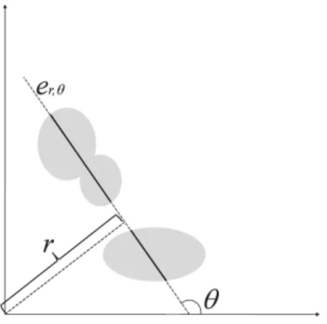
of the total projection length πθ(K) of the set K in directionθ:

L(K) =1

2

Z 2π

0 πθ(K)dθ. (9)

The total projection length is defined as πθ(K) = R∞

−∞V0(K∩er,θ)dr, i.e., as the integral of the number

of connected components of the one-dimensional intersection of K and the lines er,θ, where er,θ is

the line with direction θ _∈ [0,π) and the directed distance r _∈IR from the origin (Fig. 9). Integration is with respect to the distances r from the origin. On discretized binary images, the total projection length can be approximated by computing relative frequencies of certain pixel configurations at the phase boundary (Ohser and M¨ucklich, 2000). Based on these approximations of the total projection length in the 8 canonical directions in a 2D square lattice, the integral Eq. 9 can be numerically evaluated by means of a quadrature scheme.

Fig. 9. A polyconvex set K intersected by the line

er,θ, which has direction θ ∈[0,π) and the directed

distance r _∈ IR from the origin. In the example

depicted, the number of connected components V0(K∩

er,θ)is 2.

ACKNOWLEDGMENTS

This research was supported by the German Federal Ministry for Education and Science (BMBF) (Grant. No. 03SF0324) and by a grant from Deutsche Forschungsgemeinschaft (SFB 518, project B21). The authors thank Thomas Steinle for his help in performing parts of the tomographic reconstructions. We are also grateful to Gregory Beylkin and David Mastronarde who kindly provided the license for the fast FBP algorithm. Valuable comments by the referees and Yannick Anguy as the handling editor helped to substantially improve the manuscript.

REFERENCES

Bals S, Batenburg KJ, Verbeeck J, Sijbers J, Van Tendeloo G (2007). Quantitative three-dimensional reconstruction of catalyst particles for bamboo-like carbon nanotubes. Nano Lett7:3669–74.

Banhart J ed. (2007). Advanced tomographic methods in materials research and engineering. Oxford: Oxford University Press.

Batenburg KJ (2005). An evolutionary algorithm for discrete tomography. Discrete Appl Math151:36–54.

Baumann G, Barth A, Nonnenmacher TF (1993). Measuring fractal dimensions of cell contours: practical approaches and their limitations. In: Nonnenmacher TF, Losa GA, Weibel EA eds. Fractals in biology and medicine. Boston: Birkh¨auser, 182–9.

Buzug TM (2008). Computed tomography. Berlin: Springer. Carazo JM, Herman GT, Sorzano COS, Marabini R (2005). Algorithms for three-dimensional reconstruction from the imperfect projection data provided by electron microscopy. In: Frank J, ed. Electron tomography. 2nd ed. New York: Springer, 217–43.

Conover WJ (1971). Practical nonparametric statistics. New York: J. Wiley & Sons.

Faridani A, Finch DV, Ritman EL, Smith KT (1997). Local tomography II. SIAM J Appl Math57:1095–127. Feldkamp LA, Davis LC, Kress JW (1984). Practical

cone-beam algorithm. J Opt Soc AmA6:612–9.

Frank J (2005) Electron tomography. 2nd ed. New York: Springer.

Frost H, D¨uren T, Snurr RQ (2006). Effects of surface area, free volume, and heat adsorption on hydrogen uptake in metal-organic frameworks. J Phys Chem B

110:9565–70.

Furuie SS, Herman GT, Narayan TK, Kinahan PE, Karp JS, Lewitt RM (1994). A methodology for testing for statistically significant differences between fully 3D PET reconstruction algorithms. Phys Med Biol

39:341–54.

Gardner RJ (1995). Geometric tomography. Cambridge: Cambridge University Press.

Gilbert P (1972). Iterative methods for the three-dimensional reconstruction of an object from projections. J Theor Biol36:105–17.

Gibbons JD (1985). Nonparametric statistical inference. 2nd ed. New-York: Marcel Dekker.

Guderlei R, Klenk S, Mayer J, Schmidt V, Spodarev E (2007). Algorithms for the computation of Minkowski functionals of deterministic and random polyconvex sets. Image Vision Comput25:464–74.

methods in materials research and engineering. Oxford: Oxford University Press, 141–60.

Hansis E, Sch¨afer D, D¨ossel O, Grass M (2008). Evaluation of iterative sparse object reconstruction from few projections for 3-D rotational coronary angiography. IEEE T Med Imaging27:1548–55.

Hanson KM (1990). Method of evaluating image recovery algorithms based on task-performance. J Opt Soc Am A

7:1294–304.

Herman GT, Yeung KTD (1989). Evaluators of image reconstruction algorithms. Int J Imag Syst Tech

1:187–95.

Herman GT, Odhner D (1991). Evaluation of reconstruction algorithms. In: GT Herman, AK Louis, F Natterer eds. Mathematical methods in tomography. Berlin: Springer 215–27.

Herman GT, Kuba A eds. (2007). Advances in discrete tomography and its applications. Boston: Birkh¨auser. Herman GT (2009). Fundamentals of computerized

tomography. London: Springer.

Kak AC, Slaney M (1988). Principles of computerized tomographic imaging. New York: IEEE.

Klenk S, Schmidt V, Spodarev E (2006). A new algorithmic approach for the computation of Minkowski functionals of polyconvex sets. Comp Geom Theor Appl34:127–48.

Kuchment P, Lancaster K, Mogilevskaya L (1995). On local tomography. Inverse Probl11:571–89.

Kremer JR, Mastronarde DN, McIntosh JR (1996). Computer visualization of three-dimensional image data using IMOD. J Struct Biol116:71–6.

Lange A, Hentschel MP (2007). Direct iterative reconstruction of computed tomography trajectories (DIRECTT). International Symposium on Digital Industrial Radiology and Computed Tomography. Lyon.http://www.ndt.net/article/dir2007/papers/p6.pdf

Lange A, Hentschel MP, Kupsch A (2008). Computertomographische Rekonstruktion mit DIRECTT. MP Materials Testing 50:272–7. Patents DE 103 07 331 B4, DPMA (US 2006/0233459 A1). Lehmann EL, Romano JP (2005). Testing statistical

hypotheses. 3rd ed. New York: Springer.

Louis AK, Maass P (1993). Contour reconstruction in 3-D X-ray CT. IEEE T Med Imaging12:764–9.

Louis AK (2008). Combining image reconstruction and image analysis with an application to 2D-tomography. SIAM J Imag Sci1:188–208.

Matej S, Herman GT, Narayan TK, Furuie SS, Lewitt RM, Kinahan PE (1994). Evaluation of task-oriented performance of several fully 3D PET reconstruction algorithms. Phys Med Biol39:355–67.

Matej S, Furuie SS, Herman GT (1996). Relevance of statistically significant differences between reconstruction algorithms. IEEE T Image Process

5:554-6..

Mattfeldt T, Meschenmoser D, Pantle U, Schmidt V (2007). Characterization of mammary gland tissue using joint estimators of Minkowski functionals. Image Anal Stereol26:13–22.

Mayer J, Schmidt V, Schweiggert F (2004). A unified simulation framework for spatial stochastic models. Simul Model Pract Th12:307–26.

Mayer J (2004). A time-optimal algorithm for the estimation of contact distribution functions of random sets. Image Anal Stereol23:177–83.

Molchanov I (1997). Statistics of the Boolean model for practitioners and mathematicians. Chichester: J. Wiley & Sons.

Neuschaefer-Rube U, Neugebauer M, Ehrig W, Bartscher M, Hilpert U (2008). Tactile and optical microsensors: test procedures and standards. Meas Sci Technol

19:084010.

Ohser J, M¨ucklich F (2000). Statistical analysis of microstructures in materials science. Chichester: J. Wiley & Sons.

Ohser J, Schladitz K (2008). Visualization, processing and analysis of tomographic data. In: J Banhart, ed. Advanced tomographic methods in materials research and engineering. Oxford: Oxford University Press, 37– 105.

Park MS, Yoo SH, Lee DH (2000). Measurement of surface area in human mastoid air cell system. J Laryngol Otol

114:93–6.

Radon J (1917). ¨Uber die Bestimmung von Funktionen l¨angs gewisser Mannigfaltigkeiten. Ber Math Phys S¨achs Ges Wissen 59:262–77.

Ramachandran GN, Lakshminarayanan AV (1971). Three-dimensional reconstruction from radiographs and electron micrographs. Proc Natl Acad Sci USA 68:2236–40.

R Development Core Team (2007). R: A language and environment for statistical computing. Vienna: R Foundation for Statistical Computing.

Sandberg K, Mastronarde DN, Beylkin G (2003). A fast reconstruction algorithm for electron microscope tomography. J Struct Biol144:61–72.

Schneider R, Weil W (2008). Stochastic and integral geometry. Berlin: Springer

Shepp LA, Logan BF (1974). The Fourier reconstruction of a head section. IEEE T Nucl Sci 21:21–43.

effect of overabundant projection directions on 3D reconstruction algorithms. J Struct Biol133:108–18.. Stoeger T, Reinhard C, Takenaka S, Schroeppel A, Karg E,

Ritter B, Heyder J, Schulz H (2006). Instillation of six different ultrafine carbon particles indicates a surface area threshold dose for acute lung inflammation in mice. Environ Health Persp114:328–33.

Thiedmann R, Fleischer F, Hartnig C, Lehnert W, Schmidt V (2008). Stochastic 3D modeling of the GDL structure in PEM fuel cells based on thin section detection. J Electrochem Soc155:B391–9..