A Soft-Input Soft-Output Target Detection Algorithm for
Passive Radar
S. M. Sajjadi*, H. Khoshbin*
Abstract: This paper proposes a novel scheme for multi-static passive radar processing, based on soft-input soft-output processing and Bayesian sparse estimation. In this scheme, each receiver estimates the probability of target presence based on its received signal and the prior information received from a central processor. The resulting posterior target probabilities are transmitted to the central processor, where they are combined, to be sent back to the receiver nodes or used for decision making. The performance of this iterative Bayesian algorithm comes close to the optimal Multi-Input Multi-Output (MIMO) radar joint processing, although its complexity and throughput are much less than MIMO radar. Also, this architecture provides a tradeoff between bandwidth and performance of the system. The Bayesian target detection algorithm utilized in the receivers is an iterative sparse estimation algorithm named Approximate Message Passing (AMP), adapted to SISO processing for passive radar. This algorithm is similar to the state of the art greedy sparse estimation algorithms, but its performance is asymptotically equivalent to the more complex l1-optimization. AMP is rewritten in this paper in a new form, which could be used with MMSE initial filtering with reduced computational complexity. Simulations show that if the proposed architecture and algorithm are used in conjunction with LMMSE initial estimation, results comparable to jointly processed basis pursuit denoising are achieved. Moreover, unlike CoSaMP, this algorithm does not rely on an initial estimate of the number of targets.
Keywords: Multiple-Input Multiple-Output (MIMO) Radar, Passive Radar, Soft-Input Soft-Out (SISO) Processing, Sparse Estimation, Turbo Detection.
1 Introduction1
Passive radar has been an interesting topic of research for some decades [1-9]. Using illuminators of opportunity, it is possible to detect targets without any transmission, thus reducing system cost and probability of intercept. But there are important inherent problems in passive radar, which have reduced its real-world application.
One of the main drawbacks of passive radar is the presence of the direct-path signal, which could be more than 100 dB above the target signal echo. Passive radars usually try to use antenna design to decrease the power of the direct-path signal. Also it is shown that sparse estimation algorithms can perform better than matched-filter processing in such a situation [7-9]. The first algorithms of this kind applied to passive radar were greedy iterative algorithms, like Orthogonal Matching
Iranian Journal of Electrical & Electronic Engineering, 2012. Paper first received 16 Apr. 2012 and in revised form 10 Nov. 2012. * The Authors are with the Department of Electrical Engineering, Ferdowsi University of Mashhad.
E-mails: [email protected], [email protected].
Pursuit (OMP) [7] and CLEAN [8]. These algorithms basically consist of iteratively detecting and removing strongest echoes from the received signal. As it is stated in [9], these algorithms are not optimal and could produce poor results in realistic conditions. Thus using Basis Pursuit [10], an algorithm based on l1-norm, is proposed therein. Algorithms based on l1-norm are solved using linear programming methods, and are much more complex.
Another drawback of passive radar is its blind spots [1]. A multi-static passive radar solves this problem by using more receivers [5-6]. Each receiver could detect the targets independently and transmit the results to a center for decision-making. Alternatively, all the received signals could be transmitted to a central processor, to be jointly processed. This kind of joint processing, which is known as Input Multiple-Output (MIMO) radar [11-13], results in better detection in lower powers and overcomes target RCS fluctuations. Thus, joint processing would help reduce the coherent integration time needed to collect enough power from the weak signal echo. But the MIMO radar needs much
more bandwidth for transfer of the received signals to a central processor. Also the amount of processing needed in the central processor is orders of magnitude more than the multi-static passive radar.
To reduce the data transfer rate in the MIMO radar, [14] has proposed an algorithm based on Compressive Sensing (CS) [15]. Compressive sensing states that a unique response can be found for an under-determined sparse estimation problem, if some conditions on the sparsity and the number of available samples hold. In [14] it is proposed that the receiver throws away some of the received signal samples randomly before transmission to the central processor. The central processor applies Dantzig-Selector, another sparse estimation algorithm based on l1-norm [16], to the resulting under-determined problem to estimate the sparse vector of target RCS values. This method reduces the data transfer to the central processor, but it throws away some of the valuable signal power. This could result in larger integration times in the central processor, which is contradictory to the main justification of applying MIMO radar principle to the passive radar.
This paper proposes another algorithm for target detection in passive radar that is based on Soft-input Soft-output (SISO) processing. SISO processing was first introduced for turbo coding [17] and turbo equalization [18] to reduce the complexity of joint processing, without losing detection quality. In SISO equalization, the equalizer calculates symbol probabilities, based on the received signal and probabilities fed back from the decoder. The symbol probabilities are then transferred to the SISO decoder, which uses these probabilities and coder structure to calculate new bit probabilities. This iterative equalization and decoding method achieves near-optimal data detection in a few rounds. In this paper the same principle is applied to passive radar. SISO target detection is performed at each receiver node and the resulting posterior target probabilities are transmitted to a central processor. The central processor combines these probabilities into a joint detection probability vector, which is sent back to each node for further processing. This process is repeated until a stationary result is achieved. This scheme would have two benefits: First, the computational complexity is reduced in comparison to basic MIMO radar. Second, as the probability vectors are inherently sparse, the data throughput between the receiver nodes and the central processor decreases greatly.
A Bayesian target detection algorithm should be implemented in each receiver node of the SISO passive radar. Donoho et al have proposed such an algorithm in [19] based on belief propagation. The algorithm, called Approximate Message Passing (AMP), assumes the information transferred in the belief propagation is Gaussian, and estimates its mean and variance iteratively. The resulting algorithm is very similar to iterative soft thresholding (IST), and only includes
simple linear operations. AMP is proved [20] to be asymptotically equivalent to Basis Pursuit Denoising (BPDN) [10]. Moreover, this algorithm lends itself to usage of priors [21]. These properties have led to usage of AMP in SISO processing where the signal model is sparse. AMP has been used in [22] for SISO equalization and decoding of sparse channels, and in [23] for estimation of structured sparse signals. AMP is unique in that it resembles the greedy sparse estimation algorithms, while performing as well as the algorithms based on l1-norm.
The contributions of this paper are threefold. First, the paper proposes SISO processing to reduce complexity and bandwidth of MIMO radar. Second, the AMP algorithm is proposed to be used in passive radar to fill the gap between the greedy iterative sparse estimation algorithms and the complex algorithms based on l1-norm. Third, the AMP is adapted to be used in the SISO processing scheme and some simplifications are proposed to reduce its complexity. Also it is shown that the resulting SISO processing scheme provides tradeoffs between detection performance, in terms of false alarm rate and detection rate, and complexity.
The paper is organized as follows: In the next chapter the system model is described. Then in chapter 3, AMP algorithm and its adaptation to the MIMO passive radar is developed. In chapter 4 simulation results are reported and the algorithm is compared with the most recent developments. Finally chapter 5 concludes the paper.
2 System Model
2.1 Received Signal Model
Assume a MIMO radar system in which there are N transmitters, M receivers and T targets. In the case of passive radar, the transmitters are non-cooperative illuminators of opportunity. The signal from transmitter
n, reflected from target i and received at receiver m is modeled as:
{
j f t}
d t x att att
t
ymin()= niσmin im n( − min)exp− 2π d,min (1)
where attni and attim are respectively the attenuation of
signal from the transmitter to the target and from the target to the receiver in the free space. σmin is the RCS
of target ias viewed from receiver m with respect to the transmitter n, dmin is the total delay of the reflected
signal with respect to the direct path, and fd,min is the
target Doppler observed at receiver m with respect to the transmitter n. Considering all the signal paths, from all the transmitters and reflected from all the targets, the total signal received at receiver m equals:
∑
∑
= =
+ ⎟ ⎠ ⎞ ⎜
⎝
⎛ +
= N
n
m T
i in m mn
direct
m t y t y t n t
y
1 1
, ( ) ( ) ( )
)
( (2)
where n(t) is the additive white Gaussian noise, and
) (
, t
ydirectmn is the direct path signal from transmitter n to receiver m. We assume that the signals from various transmitters are uncorrelated due to use of some multiplexing scheme, as is common in broadcast and mobile communication systems. Therefore, the received signal in receiver m from transmitter n after sampling is modeled as:
[ ]
k y[ ]
k n[ ]
k yk
y T mn
i min mn
direct
mn = +
∑
+=1 ,
]
[ (3)
Now assume a grid on the target positions and velocities. Namely assume TG combinations of possible
target positions and velocities. ymn is rewritten as below:
[ ]
[ ]
[ ]
[ ]
[ ]
k
n
[ ]
k
k
n
s
k
y
k
y
k
y
mn t
mn
mn T
i
i in m mn
direct mn
G
+
=
+
+
=
∑
=
s
y
~
~
1 ,
(4)
where TG is the number of grid points, and []t is the
transpose operation. Also, we have
[ ]
[ ]
[ ]
[
]
′= y k y k y k
k
ymn[ ] m1n ,L, mTGn , direct,mn , 1
~
1=
+
G
T
s , and
⎩ ⎨ ⎧ =
i point grid at target No 0
i point grid at present Target 1
~
i
s (5)
Combining the RCS into ~s, and considering K consecutive time samples, the following model will result:
mn mn mn
mn A s n
y = + (6)
where Amn is a K×(TG+1) matrix, with the following values:
[ ]
[ ]
[
]
⎪⎩ ⎪ ⎨ ⎧
+ =
+ ≠ −
=
−
1 1 ,
min ,
2 min
G mn
mn
G t f j m
im ni mn
T i k
x att
T i e
d k x att att i
k d
π
A (7)
and
[ ]
⎪ ⎩ ⎪ ⎨ ⎧
+ =
+ ≠
+ ≠ =
1 1
point grid at target no and 1 0
point grid at target and 1
min
G G G
mn
T i
i T
i
i T
i i
σ
s (8)
Obviously, as the grid points are equivalent for
various transmitter-receiver pairs, the support of all
s
mnis equivalent, although their values may be different. Target detection, positioning and velocity estimation is equivalent to estimation of the support of
s
mn.l
11
s
11
y
N
1
y
l N
1
s
l
11
ω
l N
1
ω
l M1
s
1
M y
MN y
l MN s
l M1
ω
l MN
ω
( )
t y1( )
tyM l
M
p
l
1
p
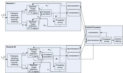
Fig. 1 The multi-static SISO passive radar, and the flow of information.
2.2 SISO Radar Structure
The structure of the multi-static passive radar proposed here is shown in Fig. 1. The radar consists of
M receiver nodes and one central processor. In each receiver node, the received signals from various transmitters are separated. The signal received from each transmitter is used in a Bayesian sparse estimation algorithm to generate a posteriori probability of target presence for that grid point. The details of the algorithm used in each node are discussed in the next chapter.
Each of the Bayesian detection algorithms generates a posterior probability vector plmn. These values can be
combined locally to obtain ωlmn, which can be used as the prior value for the next iteration. Alternatively, plmn values in each node can be compressed and transmitted to the central processor, to calculate a joint estimate of target probabilities, ωl. The values in ωl could be sent back to the receivers for the next iteration of the Bayesian sparse estimation algorithm, or be used for decision making.
Calculation of ω in both cases is the same. For the
i-th target, define tp
( )
i as presence of target at grid point i. Then:( )
(
)
( )
(
)
(
( )
)
( )
(
)
(
( )
)
(
( )
)
(
( )
)
(
)
(
1)
1 1
1
1
1 m m
1 1
not not
| |
| |
− =
− =
−
=
− ⎟ ⎠ ⎞ ⎜
⎝
⎛ −
+ ⎟ ⎠ ⎞ ⎜
⎝ ⎛
⎟ ⎠ ⎞ ⎜
⎝ ⎛ =
+ =
=
∏
∏
∏
l i N
n
l in m l
t N
n l in m
l i N
n l in m
m m
l i
p p
p
i tp p i tp p
i tp p i tp p
i tp p i tp p i tp p
ω
ω
ω
ω
y y
y y
( 9 )
The prior value of ω =ωpr
0
are set to small values for each i, so that sparsity is enforced.
The possibility of calculating ωl at each receiver locally, or joint calculation at a central processor, provides a trade-off between joint processing and data transmission. We could reduce data transmission with less joint processing, or increase the joint processing with an increased amount of data transmission. Some results on the best trade-off point are given in chapter 4. Another aspect of this two-step refinement is that the probabilities calculated in the early iterations have not converged and, as a result, are less compressible. So, these probabilities need more bandwidth for transmission to the center. This would increase the amount of transmission needed. By letting the Bayesian estimation algorithms in each receiver to converge more, the transmitted data would be more compressible, resulting in less data traffic.
3 Bayesian Sparse Estimation Algorithm 3.1 Approximate Message Passing
Approximate message passing is a Bayesian sparse estimation algorithm based on belief propagation, developed and analyzed by Donoho et al. [19-21]. The mean square error of AMP is equivalent to LASSO [24] in asymptotically large problems [20]. In this section this algorithm is briefly introduced.
AMP is based on a graphical model of the sparse estimation problem in Eq. (6), derived from decoupling of the prior information on Smn, and the conditional
distribution of the noise nmn. In the derivations in this
section, the mn subscript is omitted for the sake of simplicity.
Assume that the prior distribution of s is
( )
∏
( )
= = TG
i i i
ds d
1
α
s
α . After observing the received signal,
the following a posteriori distribution is obtained for s:
( )
∏
( )
∏
( )
= ⎟⎠ =
⎞ ⎜
⎝
⎛− −
= K
k
T
i i i
k k
G
ds y
Z d
1 1
2
2 exp
1
β
α
As s
μ (10)
where Z is a factor used to normalize μ to be a distribution function and β is a constant defining presumed sparsity. The mode of this distribution coincides with the solution of the BPDN problem:
2 2 1 2
1
minimize λs + y−As . (11)
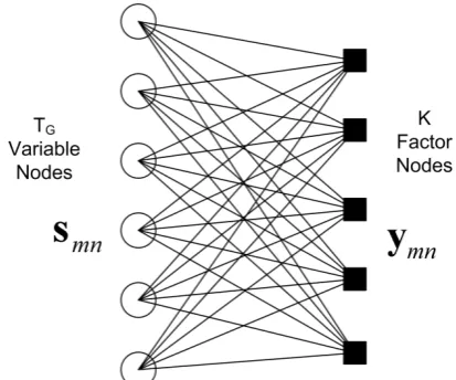
The factorized distribution in Eq. (10) can be described by a factor graph as shown in Fig. 2. There are TG "variable nodes", each node representing one of
the elements of s, and K "factor nodes", each node representing one of the K observed samples in this factor graph. Each edge on the graph means a non-zero value in the corresponding model matrix A. Each of the factors in Eq. (10) is related only to one of the nodes in the factor graph.
Fig. 2Factor graph for the posterior distribution of the signal
To obtain the posterior probability distribution of s, a belief propagation algorithm can be implemented on the factor graph, with the following measure:
(
)
( )
s x( )
sb x, b x, s d b z d
fi αi
β β ⎟ ⎠ ⎞ ⎜ ⎝ ⎛− − = 2 2 exp 1
; (12)
It is proved in [19] that the mean and variances of the messages from variable nodes to factor nodes in the
st
l iteration of the belief propagation algorithm are as follows: ⎟ ⎠ ⎞ ⎜ ⎝ ⎛ + = ⎟ ⎠ ⎞ ⎜ ⎝ ⎛ + =
∑
∑
≠ = + → ≠ = + → l K k m m l m mi l i k l K k m m l m mi l k i z A z A s γ λ β γ γ λ ; ; , 1 1 , 1 1 G F (13) where( )
(
(
)
)
( )
xb(
(
xb)
)
G b x b x F , ; ; , ; ; ⋅ = ⋅ = i i i i f Var f E. (14)
and z is the residue left from omitting the estimated signal after each iteration.
Setting z0=y, AMP would be derived as:
(
)
(
)
(
l t l)
l l l l l l l l l l l l l K K
γ
λ
γ
γ
λ
γ
λ
+ + = + + ′ + − = + + = ′ = + + − ; 1 ; ; 1 1 1 θ s G z θ s F As y z θ s F s z A θ (15)3.2 AMP with Gaussian Mixture Priors
The priors used in the basic AMP algorithm are Laplace priors which demonstrate the sparsity of the original signal. To be able to include the feedback information from the central processor, a more complex prior structure is needed. It has been proposed to use Gaussian mixtures [23], as they can accommodate the feedback probabilities besides the sparsity prior, and are also mathematically tractable.
If there is no target at point i, the distribution of si
will be a complex Gaussian distribution with zero mean and variance equal to the power of noise and interference:
( )
(
2)
, 0
; n
i i
n s CNs
Q =
σ
(16)and if there is a target, and its RCS obeys a complex Gaussian distribution with mean equal to μs and
variance equal to σrcs2, distribution of si would be:
( )
(
2)
2 2 2, ,
; s s s n rcs
i i
t s CN s
Q =
μ
σ
σ
=σ
+σ
(17)Assuming ωpr as the prior probability of target
presence at various grid points; the total Bernoulli-Gaussian distribution of si would be:
( )
(
(
)
(
)
)
⎥ ⎥ ⎦ ⎤ ⎢ ⎢ ⎣ ⎡ − + = 2 , 2 , , 0 ; 1 , ; n i i pr s s i i pr i prior s CN s CN C s pσ
ω
σ
μ
ω
(18)where C is a normalizing coefficient. With this prior probability, Eq. (12) becomes a Gaussian mixture prior equal to:
(
)
( )
(
)
⎥ ⎥ ⎥ ⎥ ⎥ ⎥ ⎥ ⎦ ⎤ ⎢ ⎢ ⎢ ⎢ ⎢ ⎢ ⎢ ⎣ ⎡ ⎟⎟ ⎟ ⎠ ⎞ ⎜⎜ ⎜ ⎝ ⎛ − − − − + ⎟⎟ ⎟ ⎠ ⎞ ⎜⎜ ⎜ ⎝ ⎛ − − − = ⎟ ⎟ ⎠ ⎞ ⎜ ⎜ ⎝ ⎛ 2 − −= −>
2 2 exp 1 2 2 exp exp , ; 2 , 2 2 , 2 2 , , 1 , 2 1 , 2 1 , , 2 i i i i i pr i i i i i pr i xi fi i i i i i i x x K x v b x s K b x s f α σ μ ω α σ μ ω β β (19) where
[
]
[
]
⎟ ⎟ ⎠ ⎞ ⎜ ⎜ ⎝ ⎛ − = − + − = = + + = + = + = − − − − − − − − − − − 4 2 2 , 1 2 2 , 1 2 1 , 2 2 2 1 , 2 1 , 1 2 2 , 2 , 1 2 1 2 1 , 1 1 2 2 2 , 1 1 2 2 1 , 1 , , , n i i i i i i i s j s i i i i i i s i s t i n i s i b x b x x b b bx b bσ
σ
β
α
β
μ
σ
μ
μ
α
β
σ
μ
β
σ
β
σ
μ
μ
β
σ
σ
β
σ
σ
(20)After some straightforward development, and by defining ⎟⎟ ⎠ ⎞ ⎜⎜ ⎝ ⎛ − = ⎟⎟ ⎠ ⎞ ⎜⎜ ⎝ ⎛− = 2 exp 2 2 exp 2 2 , 2 2 , 1 , 2 1 , i i i i Q R α πσ α πσ (21)
F, F′and Gare driven as follows [21]:
(
)
(
(
)
)
Q R Q R b x F i pr i pr i i pr i i pr i pr i i , , 2 , , 1 , , , 1 1 , ;ω
ω
μ
ω
μ
ω
ω
− + − += (22)
(
)
(
)
(
)
(
)
(
)
(
)
2 , , 2 2 , 2 2 , , 2 1 , 2 1 , , , ; 1 1 , ; i i i pr i pr i i i pr i i i pr i pr i i b x F Q R Q R b x G − − + + − + + = ω ω σ μ ω σ μ ω ω (23)(
)
(
)
i i i i i pr i i b x G b x b x F ; ,; ω , β
= ∂
∂
(24)
Finally, the slmn values resulting from AMP could
be used to calculate target probabilities based on the Gaussian assumption:
(
)
( )
( )
( )
i n i t i s mn l s Q s Q s Q l i t p P + = −= (); thiteration
min y (25)
3.3 AMP Simplification
Considering the AMP algorithm in Eq. (15), one could notice that zl+1 is mainly calculated from y, not zl. This shows that θl could be written as a function of y and θ0. Omitting the derivations, AMP could be rewritten as follows:
(
)
(
)
(
)
(
)
l l l l h l l l l l l l l l l l l l l l l l l l l l l K K K Aξ y z Aξ A s θ θ ξ θ s F s ξ θ s F θ s G θ s F s − = − + = + + ′ + = + + ′ + = + + = + + = + + − − + − ζ ζ γ λ ζ γ λ ζ γ λ γ γ λ 1 0 1 1 1 1 1 ; ; 1 ; 1 ; (26)where
ζ
−1=1,ξ−1=0,θ0=Ahy,s−1=0.In the case of matched filtering, the original AMP needs about 2KTG calculations in each iteration
(excluding the operators F, G and F΄, which are less complex). When the algorithm is rewritten as Eq. (26), preprocessing with about KTG +KTG
2
multiplications
and then about TG2 multiplications in each iteration. As
AMP usually converges very fast [19], the new algorithm's complexity is superior in one of the following situations:
- AhA≈I, thus omitting the calculation of AhAξl.
- TG <<K , so that TG <<KTG
2
and so the new method is less complex than matched filtering.
- AhA is less complex than usual matrix multiplication, or could be calculated sample by sample.
The first condition is satisfied when the simple matched filter is replaced by an adaptive filter which is calculated only once to estimate θ0. This filter could be an adaptive MMSE filter which is calculated sequentially from the time the frame starts [25]. Of course in this case AhA could not be calculated directly, but we could assume that the MMSE estimate is near-optimal, and so AhA≈I.
The second condition might happen when a target is being tracked, so that the grid points are only dense around it and are very sparse further. The last case could happen with signals like OFDM transmissions, in a slightly different signal model.
4 Simulation Results
In this section simulation results for evaluation of the proposed algorithm are presented. Two state-of-the-art algorithms are used for performance comparison with the proposed algorithm. The first one is BPDN algorithm which has been used in [9] for passive radar. BPDN, although rather complex, is one of the best sparse estimation algorithms. The second algorithm is the greedy iterative algorithms, CoSaMP [26]. For the BPDN algorithm implementation, the SPGL1 package [27] is used. For all the algorithms, a large set of examinations where performed to select the best set of parameters.
One of the most important parameters in the AMP algorithm is the variance of the interference and noise,
2
n
σ . Setting this value too low results in lots of false alarms, while too high values would reduce probability of detection. When the sequential LMMSE algorithm is used, the median of the columns of the minimum MSE matrix are used to calculate the threshold. In the case of matched filtering, we have used the signal
autocorrelation values to estimate
σ
n2 . In this case, as ll Az
θ = ′ , the variance of interference at grid point i can be written as:
2 ; 1 2 ; 1 2 int
⎭
⎬
⎫
⎩
⎨
⎧
−
⎪⎭
⎪
⎬
⎫
⎪⎩
⎪
⎨
⎧
=
∑
∑
≠ = ≠ = G G T i i i T i i iE
E
τ τ τ τ ττ τ τ
ρ
α
ρ
α
σ
(27)where ρτi is the value of the non-normalized ambiguity
function of the transmitted signal at grid point τ, when centered at grid point i. Also
⎩ ⎨ ⎧ = otherwise 0 point grid at present target
τ
σ
α
τ τ m n (28)Using the prior probabilities ωil, The resulting
calculated variance is:
{ }
(
)
[
]
∑
∑
∑
≠ = ≠ = ≠ = = − × + = = T i l i m n i T i l i l i m n i T i i E ττ τ τ
τ
τ τ τ
τ
τ τ τ
ω
σ
ρ
ω
ω
σ
ρ
α
ρ
σ
; 1 2 2 ; 1 2 2 ; 1 2 2 2 int 10 (29)
These calculations add KTG2/2 initial multiplications
to calculate ρτi, and
2
G
T more multiplications in each iteration, but they result in better target detection and lower false alarm rate.
Simulations are based on a DVB-T network, because of its vast coverage and good ambiguity function. The DVB-T transmitters use 2K Mode DVB-T with (204,188) shortened RS coding, convolutional
interleaver, 3/4 punctured convolutional code and 64-QAM modulation. To be able to implement all the algorithms, with their various degrees of complexity, a small simulation environment is considered with dimensions of 10x10 kilometers. No Doppler is assumed, and the targets are assumed to be on a grid of 12x12 equally-spaced points. Although these conditions are not realistic, they were enforced by the computational power available. All the transmitter powers are assumed equivalent.
In all the simulations, the targets are assumed to obey Swerling model type I, and the variance of the RCS values is assumed to be 10 m2. This is in contrast to [14], which considers point targets with constant RCS from all the angles, which means that all smn vectors in
Eq. (6) are equal. Using the Swerling models mean that the RCS of the target seen between each pair of transmitters and receivers is different. Thus the vectors
smn in Eq. (6) are sparse with equivalent support. Such a
problem is called a "jointly sparse", or "Multiple Measurements Vector" (MMV) problem. In this situation the Dantzig Selector algorithm in [14] is not suitable, MMV versions of the BPDN and CoSaMP algorithms are developed and used. In all the algorithms, the direct path signal is cancelled by estimating its power with a matched filter and subtracting it from the received signal.
The parameters used as the base of the comparison are detection probability and false alarm rate, with respect to the transmitter power. These parameters are obtained by averaging over 100 random geometries. In each geometry, positions of the transmitters, the receivers and the targets are selected randomly on the grid. In all the simulations, the receivers have no assumptions on the number of targets, except for CoSaMP, which needs an initial estimate of the number of targets.
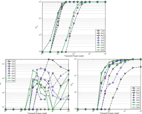
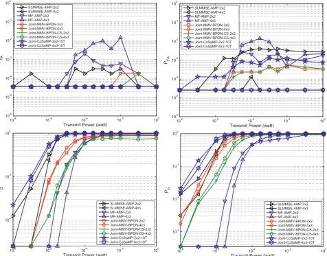
Fig. 3 Effect of number of iterations in each receiver (the second number in the legends), and number of transmissions to the central processor (the first number in the legends). Up: MMSE-AMP detection rate; Bottom Left: MF-AMP false alarm rate; Bottom Right: MF-AMP detection rate.
Two set of simulations, one with 2 targets present and the other with 10 targets present, have been performed. The detection threshold is set on probability of 0.1. Simulation results not presented here show that a slight change (about 3 dB) in this value does not have any significant effect on the results.
To see the trade-off between data transmission and estimation quality, a scenario with 3 transmitters, 4 receivers and 10 targets is considered. The number of iterations of AMP algorithm on each receiver, before transmitting the current results to the central processor was varied. Also the number of retransmissions from the central processor to each transmitter was changed too. The results are shown in Fig. 3. In these simulations, the false alarms for the MMSE-AMP algorithm were negligible and are so omitted.
As is observed in Fig. 3, it is essential to have at least one retransmission from the central processor to the receivers. This could improve the results by more than 10 dB. More retransmissions result in less improvement each time.
Increased number of iterations in each receiver results in better detection, so that the detection probability with 4 iterations in each receiver is better than those with 3 or 2 iterations. This could be attributed to extraction of more power from each target reflection, which would cause the probabilities to go higher. But at the same time, more iteration in each receiver, above 3, cause higher false alarm rate in higher powers. In fact the receivers need the first 2 iterations to reach a good starting point, and thereafter try to extract more signals based on that starting point. Without information from the other receivers, they tend to extract more and more targets, to reduce the residue power. Thus, although they are able to detect targets better, they tend to have more false alarms too. This didn't happen in the MMSE-AMP algorithm, because the initial MMSE had suppressed much of the correlations, before AMP iterations. As false alarm rate is usually given predominance, and the difference in detection performance is not huge, we have chosen to have 3 iterations in each receiver, and at least 4 data transfers to the central processor.
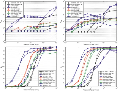
Fig. 4 PD and PFA for various algorithms, in one-receiver scenario: Left Up: 2 targets PFA; Right Up: 10 targets PFA; Left Down: 2 targets PD; Right Down: 10 targets PD.
Fig. 5 PD and PFA for various algorithms, in multiple-receiver scenario: Left Up: 2 targets PFA; Right Up: 10 targets PFA; Left Down:
2 targets PD; Right Down: 10 targets PD.
In the next simulation, we have analyzed the effect of number of transmitters and number of receivers on detection and false alarm quality. In Fig. 4, the detection and false alarm rates of one receiver, with various numbers of transmitters, are plotted.
When there is only one receiver, the AMP-based algorithms show the worst detection performance. Between them, MF-AMP starts to detect in lower transmit powers, but MMSE-AMP has better detection probability in higher powers. The difference between BPDN with complete data and MMSE-AMP is about 15 dB in mid-range SNRs in the 10 target scenario, while the CS version of BPDN - which uses 50% of the acquired samples - is only 3dB below BPDN. But in the higher SNRs, MMSE-AMP is the best algorithm, detecting all the present targets, while MMV-BPDN and MMV-CoSaMP could not detect all the targets with 2 transmitters.
As for false alarm rate, performance of MF-AMP is again the worst, so much that it might become useless in some cases. MMSE-AMP also has high false alarm rate with 2 transmitters, but this rate is reduced with more
transmitters. This observation is in line with previous analysis [20] which states that IST algorithms tend to have high false alarm rate. The false alarm rate increases with the number of targets in all the algorithms. The best algorithm in this regard is CoSaMP, in which the maximum number of targets is a predefined constant, thus limiting the allowed false alarm rate. MMSE-AMP is the next, followed by full-sample and CS versions of BPDN.
To demonstrate the MIMO system, 2 scenarios, one with 2 receivers and 2 transmitters, and the other with 4 receivers and 3 transmitters are considered. The results are provided in Fig. 5.
As is shown in Fig. 5, in the 3Tx-4Rx scenario, MMSE-AMP has the best false alarm rate, and its detection performance is second to the best algorithm - CoSaMP. Although MF-AMP has yet the worst performance, both its false alarm rate and detection performance are improved considerably with respect to the one-receiver scenario. The detection probability of MF-AMP in the 2-target, 3Tx-4Rx scenario is equal to
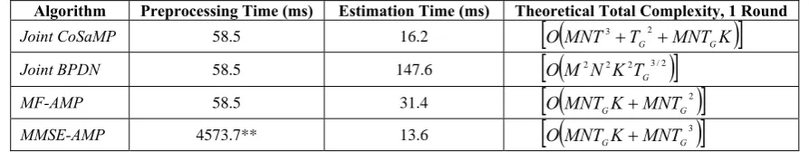
Table 1 The empirical and analytical complexities of various algorithms.
Algorithm Preprocessing Time (ms) Estimation Time (ms) Theoretical Total Complexity, 1 Round
Joint CoSaMP 58.5 16.2
[
O(
MNT3+TG2+MNTGK)
]
Joint BPDN 58.5 147.6
[
(
2 2 2 3/2)
]
G
T K N M O
MF-AMP 58.5 31.4
[
O(
MNTGK+MNTG2)
]
MMSE-AMP 4573.7** 13.6
[
O(
MNTGK+MNTG3)
]
CS-BPDN. Obviously, addition of transmitter/receiver pairs helps AMP algorithms to achieve performances on par or better than the best algorithms available.
A measure of the complexity of the algorithms is also needed to be able to compare the algorithms. Both analytical and empirical results on the complexity of the algorithms are given in Table 1. The empirical results are calculated by averaging run time of the simulations on a PC (Core-i7 6760, 4 GB RAM).
As the SPGL1 package does not state any complexity calculations, the single-round complexity of BPDN algorithm is estimated based on the L1-LP implementation, analyzed in [28]. Note that the number of iterations needed for BPDN to converge is an order of magnitude greater than the other algorithms. In calculation of the complexity of MMSE-AMP, sequential update of the SLMMSE estimator is considered. For CoSaMP, the predetermined number of targets, shown by
T
c, is also needed to calculate the complexity.The empirical results in Table 1 show that the preprocessing time for MMSE-AMP is two orders of magnitude greater than the other algorithms. This is because of our SLMMSE implementation, which uses a new snapshot of data in each simulation round. In a realistic scenario, this algorithm changes to Kalman filtering, and the difference is much smaller. The processing time of the CoSaMP and MMSE-AMP is near each other, while MF-AMP takes more time. This difference is also due to implementation, as the MF-AMP algorithm is implemented without the simplifications in chapter 3-3. The BPDN algorithm is the most complex, and needs the most amount of time.
In a real-world scenario, both K and TG would be
much larger than the simulations. In this case, complexity of MF-AMP would be the least, followed by CoSaMP, MMSE-AMP and BPDN. If the SLMMSE algorithm could be implemented with lower complexity, the complexity of MMSE-AMP would become nearly equivalent to CoSaMP. This could be the case in OFDM-based modulations, where frequency domain estimation based on FFT could be used. Anyhow, it should be noted that CoSaMP needs an accurate initial estimate of the number of targets, but AMP-based algorithms don't need such an estimate and are insensitive to the initial estimate of sparsity value.
5 Conclusion
This paper has proposed a new architecture for multi-static passive radar, based on input soft-output processing and Bayesian sparse estimation. This combination has two benefits: First, it reduces the bandwidth needed for joint processing while achieving comparable results. Second, it could cope with the direct-path signal through sparse estimation.
The Bayesian sparse estimation algorithm used in the receiver nodes is AMP, which is adapted to use Gaussian mixture priors, to be able to accept the probabilities fed back from the central processor. Also the algorithm is rewritten so that it can be used with MMSE initial filtering, or any other adaptive filter, while the complexity is not increased substantially.
The simulations have shown that the algorithm is inferior to joint processing when there is only one receiver, but when the number of transmitters and receivers increase, it can achieve results equal to joint processing with MMV-BPDN algorithm. The algorithms performance is below CoSaMP, especially at false alarm rate, but it should be noted that CoSaMP needs an initial estimate on the number of targets, while the proposed algorithm does not.
Also it is shown that more iterations in each receiver node before transmission of the data for the central processor increases both detection and false alarm rate. The best results are achieved when 2 or 3 iterations are run in each receiver, before probability transmission. This also reduces the required bandwidth, by generating more compressible probabilities.
Future work includes study of various parts of this system. One of the interesting areas of research would be utilization of the DVB signal structure for frequency domain filtering. Also the algorithms in the central processor can be extended to target acquisition or tracking.
References
[1] Griffiths H. D., Garnett A. J., Baker C. J. and Keaveney S., “Bistatic radar using satellite-borne illuminators of opportunity”, in Proceedings of
International Conference on Radar, Radar 92, Brighton, UK, pp. 276-279, Aug. 1992.
[2] Lanterman A. D., “Tracking and recognition of airborne targets via commercial television and FM radio signals”, in Proceedings of SPIE
Acquisition, Tracking and Pointing XIII Conference, Orlando, FL, pp. 189-198, Apr. 1999.
[3] Griffiths H. D. and Baker C. J., “Passive coherent location radar systems. Part 1: Performance prediction”, IEE Proceedings on
Radar, Sonar and Navigation, Vol. 152, No. 3, pp. 153-159, June 2005.
[4] Lauri A., Colone F., Cardinali R., Bongioanni C. and Lombardo P., “Analysis and Emulation of FM Radio Signals for Passive Radar”, in
Proceedings of IEEE Aerospace Conference, Big Sky ,MT, pp. 1-10, June 2007.
[5] Baker C. J. and Griffiths H. D., “Bistatic and Multistatic Radar Sensors for Homeland Security”, Advances in Sensing with Security
Applications, edited by Jim Byrnes and Gerald Ostheimer, Dordrecht, The Netherlands: Springer, Vol. 2, pp. 1-22, 2006.
[6] Lesturgie M., “Use of dynamic radar signature for multistatic passive localisation of helicopter”,
IEE Proceedings on Radar, Sonar and Navigation, Vol. 152, No. 6, pp. 395-403, Dec. 2005.
[7] Berger C. R., Zhou Shengli and Willett P., “Signal extraction using compressed sensing for
passive radar with OFDM signals”, in
Proceedings of 11th International Conference on Information Fusion, Cologne, Germany, pp. 1-6, June-July 2008.
[8] Kulpa K., “The CLEAN type algorithms for radar signal processing", in Proceedings of
Microwave, Radar and Remote Sensing, MRRS 2008, Kiev, Ukraine, pp. 152-157, Sep. 2008. [9] Berger C. R., Demissie B., Heckenbach J.,
Willett P. and Shengli Zh., “Signal processing for passive radar using OFDM waveforms",
IEEE Journal on Selected Topics in Signal Processing, Vol. 4, No. 1, pp. 226-238, Feb. 2010.
[10] Chen S. S., Donoho D. L. and Saunders M. A., “Atomic decomposition by basis pursuit”, SIAM
Journal on Scientific Computing, Vol. 20, No. 1, pp. 33-61, 1999.
[11] Fishler E., Haimovic A., Blum R., Chizik D., Cimini L. and Valenzuela R., “MIMO RADAR: an idea whose time has Come”, inProceedings
of IEEE Radar Conference, pp. 71-78, Apr. 2004.
[12] Fishler E., Haimovic A., Blum R. S., Cimini L. J., Chizik D. and Valenzuela R. A., “Spatial diversity in radars-models and detection performance”, IEEE Transactions on Signal
Processing, Vol. 54, No.3, pp. 823-838, Mar. 2006.
[13] Merline A. and Thiruvengadam S. J., “Power allocation strategies for mimo radar waveform design”, Iranian Journal of Electrical and
Electronic Engineering, Vol. 7, No. 2, pp. 106-111, 2011.
[14] Yu Y., Petropulu A. P., and Poor H. V., “MIMO radar using compressive sampling”, IEEE
Journal on Selected Topics in Signal Processing, Vol. 4, No. 1, pp. 146-163, Feb. 2010.
[15] Donoho D. L., “Compressed sensing”, IEEE
Transactions on Information Theory, Vol. 52, No. 4, pp. 1289-1306, Apr. 2006.
[16] Candes E. and Tao T., “The Dantzig selector: statistical estimation when p is much larger than n”, Annals of Statistics, Vol. 35, No. 6, pp. 2313-2351, Dec. 2007.
[17] Berrou C., Glavieux A. and Thitimajshima P., “Near Shannon limit error-correcting coding and decoding: turbo codes”, in Proceedings of
International Conference on Communications, ICC93, Geneva, Switzerland, Vol. 2, pp. 1064-1070, 1993.
[18] Douillard C., Jézéquel M., Berrou C., Picart A., Didier P. and Glavieux A., “Iterative correction of intersymbol interference: turbo equalization”,
European Transactions on Telecommunications,
Vol. 6, No. 5, pp. 507-511, Sep-Oct 1995. [19] Donoho D. L., Maleki A. and Montanari A.,
“Message passing algorithms for compressed sensing”, Proceedings of the National Academy
of Sciences, Vol. 106, No. 45, pp. 18914-18919, Nov. 2009.
[20] Montanari A., “Graphical models concepts in compressed sensing”, Compressed Sensing:
Theory and Applications, chapter 9, 1th edition, edited by Y. C. Eldar and G. Kutynok, Cambridge, UK: Cambridge University Press, 2012.
[21] Donoho D. L., Maleki A. and Montanari A., “Message passing algorithms for compressed sensing: I. motivation and construction”, in
Proceedings of IEEE Information Theory Workshop, ITW, Cairo, Egypt, pp 1-5, Jan. 2010. [22] Schniter P., “A message-passing receiver for
BICM-OFDM over unknown clustered-sparse channels”, IEEE Journal on Selected Topics in
Signal Processing, Vol. 5, No. 8, pp 1462-1474, Dec. 2011.
[23] Schniter P., “Turbo reconstruction of structured sparse signals”, in Proceedings of 44th Annual
Conference on Information Sciences and Systems, Princeton, pp 1-6, Mar. 2010.
[24] Tibshirani R., “Regression shrinkage and selection via the LASSO”, Journal of the Royal
Statistical Society, Vol. 46, No. 1, pp. 267-288, 1996.
[25] Kay S. M., Fundamentals of Statistical Signal
Processing, Englewood Cliffs, NJ: Prentice Hall, 1th edition, Vol. I: Estimation Theory, 1993. [26] Needell D. and Tropp J. A., “CoSaMP: iterative
signal recovery from incomplete and inaccurate
samples”, Applied and Computational Harmonic
Analysis, Vol. 26, No. 3, pp. 301-321, 2009. [27] Friedlander M. P. and Van den Berg E., SGPL1:
A solver for large-scale sparse reconstruction, May 2009, [Online]. Available: http://www.cs.ubc.ca/labs/scl/spgl1/index.html. [28] Nesterov I. E., Nemirovskii A. S., and Nesterov
Y., Interior-Point Polynomial Algorithms in
Convex Programming, Philadelphia, USA: SIAM, 1994.
Seyyed Mohammad Sajjadi received his B.Sc. degree in Electrical Engineering in 2003 from Ferdowsi University, Mashhad, Iran and M.Sc. degree in Communication Engineering in 2006 from Iranian University of Science and Technology, Tehran, Iran. He's now a Ph.D. candidate at the Department of Electrical and Computer Engineering, Ferdowsi University, Mashhad, Iran. His research interests include advanced signal processing and estimation algorithms, Radar and electronic support systems.
Hossein Khoshbin received his B.Sc. degree in Electronics Engineering and his M.Sc. degree in Communications Engineering in 1985 and 1987, respectively, both from Isfahan University of Technology, Isfahan, Iran. He received his Ph.D. degree in Communications Engineering from the University of Bath, UK, in 2000. He is currently an assistant professor at the Department of Electrical and Computer Engineering, Ferdowsi University, Mashhad, Iran. His research interests include communication theory and digital and wireless communications.