CONTINUOUS DISCRETE VARIABLE OPTIMIZATION OF
STRUCTURES USING APPROXIMATION METHODS
E. Salajegheh, J. Salajegheh and A. Heidari
Department of Civil Engineering, University of Kerman Kerman, Iran, [email protected]
(Received: July 21, 2002 – Accepted in Revised Form: June 10, 2004)
Abstract Optimum design of structures is achieved while the design variables are continuous and discrete. To reduce the computational work involved in the optimization process, all the functions that are expensive to evaluate, are approximated. To approximate these functions, a semi quadratic function is employed. Only the diagonal terms of the Hessian matrix are used and these elements are estimated from the first derivatives that are available from the previous iterations. The second order approximation is obtained for both direct and reciprocal approximations. In addition, a hybrid form of the approximation is introduced. With the help of this approximation, the continuous optimization is obtained. The results are used as the starting point for the discrete optimization. A new penalty function is introduced for discrete optimum design and the discrete variables are obtained in conjunction with the same function approximation. Examples are given and the numerical results are discussed.
Key Words Continuous Optimization, Discrete Optimization, Approximation Concepts, Penalty Functions
ﻩﺪﻴـﻜﭼ
ﻩﺪﻴـﻜﭼ
ﻩﺪﻴـﻜﭼ
ﻩﺪﻴـﻜﭼ
ﺖﺳﺍﺮﻈﻧﺩﺭﻮﻣﻪﺘﺴﺴﮔﻭﻪﺘﺳﻮﻴﭘﻱﺎﻫﺮﻴﻐﺘﻣﺯﺍﻩﺩﺎﻔﺘﺳﺍﺎﺑﺎﻫﻩﺯﺎﺳﺔﻨﻴﻬﺑﺡﺮﻃﻪﻟﺎﻘﻣﻦﻳﺍﺭﺩ
.
ﺶﻫﺎﻛﻱﺍﺮﺑ
ﺪﻧﻮﺷﻲﻣﻩﺩﺯﺐﻳﺮﻘﺗ،ﺖﺳﺍﺮﻴﮔﺖﻗﻭﺎﻬﻧﺁﺔﺒﺳﺎﺤﻣﻪﻛﻲﻌﺑﺍﻮﺗﻲﻣﺎﻤﺗﻱﺯﺎﺳﻪﻨﻴﻬﺑﺔﺳﻭﺮﭘﺭﺩﺕﺎﺒﺳﺎﺤﻣ
. ﺐﻳﺮﻘﺗﻱﺍﺮﺑ
ﺩﻮﺷﻲﻣ ﻩﺩﺎﻔﺘﺳﺍﻭﺩﻪـﺟﺭﺩﻪﺒـﺷﻊﺑﺎـﺗﻚـﻳﺯﺍ،ﻊـﺑﺍﻮﺗﻦـﻳﺍ
. ﺎﻬﻨﺗ
ﺎﺑﻭﻩﺪﺷﻩﺩﺎﻔﺘﺳﺍﻥﺎﻴﺴﻫﺲﻳﺮﺗﺎﻣﻱﺮﻄﻗﺕﻼﻤﺟ
ﺩﻮﺷﻲﻣﻪﺘﺧﺎﺳﻩﺪﻣﺁﺖﺳﺪﺑﻞﺒﻗﺭﺍﺮﻜﺗﺯﺍﻪﻛﻝﻭﺍﻖﺘﺸﻣﺯﺍﻩﺩﺎﻔﺘﺳﺍ
.
ﺩﻮﺷﻲﻣﻪﺘﺧﺎﺳﺰﻴﻧﺐﻳﺮﻘﺗﻲﺒﻴﻛﺮﺗﻊﺑﺎﺗﻚﻳ
.
ﺎﺑ
ﻱﺯﺎﺳﻪﻨﻴﻬﺑﻉﻭﺮﺷﺔﻄﻘﻧﻥﺍﻮﻨﻌﺑﻩﺪﻣﺁﺖﺳﺪﺑﺞﻳﺎﺘﻧﻭﻩﺪﻣﺁ ﺖﺳﺪﺑﻪﺘﺳﻮﻴﭘﺔﻨـﻴﻬﺑﺡﺮـﻃﺎـﻫﺐـﻳﺮﻘﺗﻦـﻳﺍﺯﺍﻩﺩﺎﻔﺘـﺳﺍ
ﺮﮔﺮـﻈﻧﺭﺩﻪﺘـﺴﺴﮔ
ﺩﻮﺷﻲـﻣﻪﺘـﻓ
. ﻪﺘﺴﺴﮔﺔﻨﻴﻬﺑﺮﻳﺩﺎﻘﻣﻭﻩﺪﺷﺩﺎﺠﻳﺍﻪﺘﺴﺴﮔﺔﻨﻴﻬﺑﺡﺮﻃﻱﺍﺮﺑﻱﺪﻳﺪﺟﻲﺘﻟﺎﻨﭘﻊﺑﺎﺗ
ﺩﻮﺷﻲﻣﻪﺒﺳﺎﺤﻣﻲﺒﻳﺮﻘﺗﺵﻭﺭﺯﺍﻩﺩﺎﻔﺘﺳﺍﺎﺑﻞﺒﻗﺪﻨﻧﺎﻤﻫ
.
ﺩﻮﺷﻲﻣﻥﺎﻴﺑ ﻝﺎﺜﻣﺪﻨﭼﻱﺩﺪﻋﺞﻳﺎﺘﻧ
.
1. INTRODUCTION
The idea of approximation concepts is now well established in numerical optimization techniques. The optimum design procedure requires the evaluation of the objective function and the constraints at a number of design points. The evaluation of some of the functions such as member forces, displacements, frequencies are time consuming. These functions are approximated and an approximate design problem is solved with move limits. The results are employed as a starting point for the next design iteration. The process is continued until the optimum design process
indicate that the number of design iterations is decreased when member forces are taken as the intermediate responses. This is basically due to the fact that the variation of forces is not very sensitive to the cross sectional properties.
Some midrange approximations were proposed by using two-point approximation [4]. The approximate functions were considered linear or quadratic by considering some non-linearity indices. The indices were selected from the data available in the previous iterations. A three-point function approximation was introduced by using the information of three consecutive design points [5]. In all the multi-point approximation, the unknown coefficients should be evaluated by solving some algebraic equations and in some cases numerical errors may encounter.
A quadratic function approximation was outlined in which all the elements of the Hessian matrix were estimated from the existing data [6]. In fact, an approximate Hessian matrix was developed based on the first derivatives. This approach is effective for design optimization as it reduces the design cycles. However, for all the constraints under consideration, the Hessian matrices must be created and stored. For further discussion of the approximation concepts Ref. [7] can be consulted.
As far as the discrete variable optimization is concerned, less research work has been carried out. Practical and efficient methods of optimum design of structures is based on choosing the design variables from a set of available values, while the computational work involved in the design process is reduced as much as possible. There are several methods for optimum design of structures with discrete variables such as branch and bound, duality theory, penalty functions, genetic algorithms, simulated annealing, etc. Each of the methods has some limitations and difficulties [8]. Among these methods, penalty functions are easy to implement and if they are combined with approximation concepts, efficient methods for both continuous and discrete optimization can be achieved. There are various techniques for employing the penalty functions for continuous optimization. However, a few penalty functions exist for the solution of problems with discrete variables. In the literature, a sine-function [9] and a quadratic function [10] have been introduced in
this regard. These methods have been combined with approximation of structural responses to enhance the efficiency of the methods [11-13]. In the present work, a semi quadratic function is developed in which only the diagonal elements of the Hessian matrix are estimated. The diagonal elements are evaluated by matching the first derivatives of the function with those of the previous iteration. Explicit relations are obtained to find the necessary unknowns, thus numerical procedures are not necessary to evaluate the second derivatives. The function is expressed in terms of the direct variables as well as the reciprocal variables. The necessary criteria are established to create a hybrid form of the direct and reciprocal approximations. In addition, a new penalty function is proposed for discrete optimization. The process of discrete variable optimum design is also combined with the function approximation in order to reduce the number of iterations.
2. FUNCTION APPROXIMATION
Given a function G(X), the quadratic approximation with the diagonal elements of the Hessian matrix is expressed as
) x )(x (X G 2 1
) x )(x (X G ) (X G (X) G
n
1 i
2 1i i 1 ii ,
n
1
i i, 1 i 1i 1
Q Q
∑
∑
= =
− +
− +
=
(1)
where X=[x1, x2, …, xi, …, xn] is the vector of design variables with n variables and X1 is the current design point. x1i is the ith element of X1. The notations G,i and G,ii represent the first and second derivatives, respectively. The subscript Q reflects the quadratic approximation. The quadratic reciprocal approximation with the use of intermediate variables
x 1 y
i
i = (2)
into Equation 1
∑
∑
= = − + − − + = n 1 i 2 i 1i 2 1i i 1 ii , n 1 i 1 1i i 1i 1i i 1 i, 1 Q QR ) x x ( ) x )(x (X G 2 1 ) x x (2 x x ) x )(x (X G ) (X G (X) G (3)First subtracting Equation 1 from Equation 3 establishes the conservative approximation, which is a hybrid form of Equations 1 and 3
∑
∑
= = − − − + − − − − = − n 1 i 2 1i i 2 i 1i 2 1i i 1 ii , n 1 i i 1i 1 1i 1i i 1i i 1 i, QR Q ] ) x (x ) x x ( ) x )[(x (X G 2 1 ] x x ) x x )(2 x (x ) x )[(x (X G (X) G (X) G (4) After some mathematical manipulationEquation 4 can be expressed as
∑
= − + − − = − n 1 i 2 1i 2 i 1 ii , 1i i 1 i, 2 i 1i i QR Q )] x )(x (X G 2 1 ) x )(x (X [G ) x x x ( G G (5) Equation 5 can be shown as∑
−=
− 2 i
i 1i i QR
Q ) . α
x x x ( G G (6) where ) x )(x (X G 2 1 ) x )(x (X G
αi = i, 1 i− 1i + ,ii 1 i2− 1i2 (7) It can be seen that the sign of (GQ-GQR) depends only on αi. Suppose that G(X) represents a constraint of the form G(X)≤0, then
If αi≤0 implies GQ≤GQR
Thus GQR is more conservative (less negative) than GQ. In this case GQR is more effective. On the other hand, if αi >0, then the use of GQ will be more conservative. Thus the criteria for the conservative
(hybrid) approximation can be stated as If αi≤0 use GQR
Otherwise use GQ.
3. ESTIMATION OF SECOND ORDER DERIVATIVES
The evaluation of the exact second order derivatives is time consuming. The approximate values of G,ii are found from the condition that the first derivatives of G(X) match those of GQ or GQR at the previous design point X0. Therefore depending on the sign of αi the first derivatives of Equation 1 or Equation 3 is matched with that of the previous point as follows:
(a) If αi>0, by using Equation 1, ) x )(x (X G ) G(X ) (X
Gi, 0 = 1 + ,ii 1 01− 1i (8)
yields 1i 0i 1 i, 0 i, 1 ii , x x ) (X G ) (X G ) (X G − −
= (9)
(b) if αi≤0, by using Equation 3 after the necessary manipulation ) x (x x ) (X )G 2x (3x x ) (X G x ) (X G 1i 0i 3 1i 1 i, 1i 0i 2 1i 0 i, 3 0i 1 ii , − − − = (10) It can be seen from Equations 9 and 10 that for
the evaluation of the second derivatives, only the first derivatives of the function under consideration are required at two design points. It is to be mentioned that in the first iteration a linear function approximation must be used.
4. CONTINUOUS OPTIMIZATION
Suppose a constrained optimization problem with m inequality constraints is expressed as
j=1,m represent the constraints. Penalty function methods are employed to solve the optimization problem. This can be achieved by solving the following unconstrained problems
.... , r , r r rP(X) F(X) r) X, (
Minimizeφ = + = 1 2 (12)
where φ is an auxiliary function, r is the penalty multiplier and P(X) is the imposed penalty function which is the function of the constraints. Any appropriate penalty function can be used for continuous optimization. In this work a quadratic extended interior penalty function has been employed [14]. By changing the value of r the minimum of φ approaches the minimum of F. The main steps for the solution of this problem in conjunction with approximation concepts can be summarized as follows:
(a) Perform a finite element analysis of the structure and evaluate all the structural responses such as element forces, nodal displacements, etc.
(b) Find the first derivatives of the necessary responses with respect to the intermediate variables and establish the approximate relations for the responses under consideration. (c) Formulate the approximate optimization
problem and evaluate the initial value of multiplier r. By gradually reducing the value of r, solve the approximate problems until the continuous problem converges.
(d) If the overall design optimization has not converged then update the analysis model and go to step (a).
5. DISCRETE OPTIMIZATION
The results of the continuous optimization are used as the starting point for the discrete variable optimization. To perform the discrete optimization, now the following problem is considered:
.... , s , s s constant : r sQ(X) rP(X) F(X) s) r, X, ( Minimize 2 1 = + + = φ (13)
in which Q(X) is the imposed penalty function for
discrete variables for which the following new function is presented:
1) -e ( Q(X) n β.q(x)
1 i
∑
=
= (14)
where ) d -(d ) x -)(d d -x ( q(x) l i u i i u i l i i γ
= (15)
and dli and dui are lower and upper discrete values for xi. The value of γ can be taken as either of 0, 1 and 2, depending on the space of discrete values. A suitable value of γ can be considered as 2. Equation 14 can be scaled such that the value of Q(X) at midpoint becomes unity, i.e.
)
d
(d
2
1
at x
1
(X)
Q
u i l ii
=
+
=
which yields β = 2.7726 for γ = 2. The numerical results indicate that this form of scaling produces a smooth function and thus makes the discrete variable optimization easier. In addition, the proposed function is parameter independent. In this step the multiplier r is kept constant and by changing s, the discrete variable optimization is achieved for one design cycle. The numerical results show that the performance of the function is better than the existing functions. The nature of the function is such that it changes smoothly at the discrete points. The main steps in the discrete optimization are as follows:
(a) Repeat similar Steps a and b in the process of continuous optimization to establish the approximate discrete design problems.
(b) Freeze the multiplier r and find the initial value of the multiplier s. Solve the approximate design problems by gradually increasing the multiplier s, until the discrete problems converge. Check if the solution is feasible and discrete, if it is not feasible, increase r and reinitialize s and go to Step a.
6. INITIAL VALUES OF MULTIPLIERS r AND s
The multiplier r is only used for the continuous optimization. The necessary condition for φ(X, r) represented by Equation 12 to be minimized is that the first partial derivatives must vanish. Therefore a suitable choice for the initial value of r would be given by the r that minimizes the magnitude of the squire of the gradient of φ (X, r) at the starting point X0, that is
) (X P r ) (X F min r)
, (X
φ , 0 , 0 2
r 2 0
, = + (16)
where φ,(X0,r) 2denotes the Euclidean norm of φ,(X0,r) and φ,(X0,r) is the gradient of φ(X0,r). Then the value of r can be obtained from Equation 16 as
) (X P
) (X P ) (X F
r 2
0 ,
0 , T 0 ,
−
= (17)
Equation 17 can be used providing it yields r>0. Because of the initial value of X0, it may happen that r < 0. In such a case either X0 may be changed or the initial value of r can be chosen in such a way that at X0, the two terms F(X) and r P(X) do not differ greatly in value. Hence, a reasonable value of r can be obtained when
) )/P(X F(X r ) P(X r )
F(X0 = 0 → = 0 0 (18)
The same approach can be argued to estimate
the initial value of s [11]. Thus
) (X Q
) (X Q ) (X F
s 2
0 ,
0 , T 0 ,
−
= (19)
provided s>0, otherwise s=F(X0)/Q(X0).
7. NUMERICAL RESULTS
A computer program has been developed based on the preceding discussion. In this study the results of four examples are presented. To compare the results, the examples are solved by the following methods:
1. Linear Approximation (LA): In this method only the first two terms of the Taylor series are chosen. For stress constraints, the direct approximation and for displacement constraints the reciprocal approximations are employed. 2. Quadratic Approximation (QA): In this method
the first three terms of the Taylor series expansion with diagonal Hessian matrix are used. Again for stress constraints the direct quadratic approximation (Equation 1) and for displacements the reciprocal quadratic approximation (Equation 3) are considered. 3. Hybrid Linear Approximation (HLA): The
hybrid approximation presented in Ref. [15] is employed. In this method, based on the sign of the first derivatives, the direct or reciprocal approximation is used.
4. Hybrid Quadratic Approximation (HQA): The method outlined in the present study.
In all cases, the member forces are first approximated and then the approximate stress constraints are established [16]. The initial move limit is considered as 90% and is gradually reduced by 10% in each iteration.
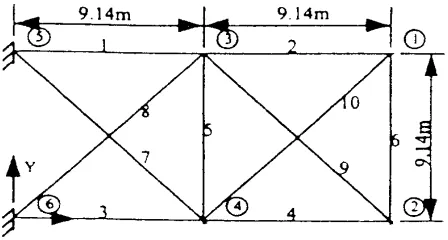
7.1. Problem 1. Ten-Bar Truss
The standard test problem shown in Figure 1 is solved with stress and displacement constraints. The material properties are given as Young’s modulus, E = 6.9×10¹⁰ N/m2, weight density,N/m2 for all members. One load case is considered as P2y=P4y=-4.45×10⁵ N. In addition to the stress constraints, displacement limits of ±5.08×10⁻² m are imposed on the vertical direction of each joint. The cross-sectional areas of members are considered as design variables. The initial value and minimum size limits are 6.45×10⁻³ m2 and
6.45×10⁻⁵ m2, respectively. The set of available discrete values for the cross-sectional areas is
{
0.645, 1, 5, 10, 15, 20, 25, ...}
(cm )Ai∈ 2
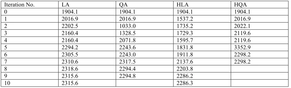
Iteration histories of the above mentioned four TABLE 1. Iteration Histories of 10-bar Truss for Continuous Variables (Weight: Kg).
Iteration No. LA QA HLA HQA
0 1904.1 1904.1 1904.1 1904.1
1 2016.9 2016.9 1537.2 2016.9
2 2202.5 1033.0 1735.2 2022.1
3 2160.4 1328.5 1729.3 2119.6
4 2160.4 2071.8 1595.7 2119.6
5 2294.2 2243.6 1831.8 3352.9
6 2305.5 2243.0 1911.8 2298.2
7 2310.6 2317.5 2137.6 2298.2
8 2318.6 2294.4 2203.8
9 2315.6 2294.8 2286.2
10 2315.6 2286.3
TABLE 2. Iteration Histories of 10-bar Truss for Discrete Variables (Weight: Kg).
Iteration No. LA QA HLA HQA
1 2315.8 2318.9 2293.6 2334.5
2 2326.6 2322.8 2303.8 2335.1
3 2322.2 2332.7 2310.8 2335.1
4 2319.3 2342.4 2321.8
5 2317.2 2344.3 2328.6
6 2317.2 2344.3 2328.6
TABLE 3. Optimum Design for 10-bar Truss (Continuous): cm2.
Member LA QA HLA HQA
1 181.89 180.59 180.37 189.02
2 15.08 2.85 3.47 9.10
3 161.20 154.39 153.18 158.38
4 82.84 86.55 95.79 87.32
5 9.30 2.84 2.47 4.90
6 0.645 1.04 1.43 0.766
7 73.23 67.22 54.28 59.33
8 116.60 132.54 136.91 129.69
9 116.73 133.31 133.98 126.25
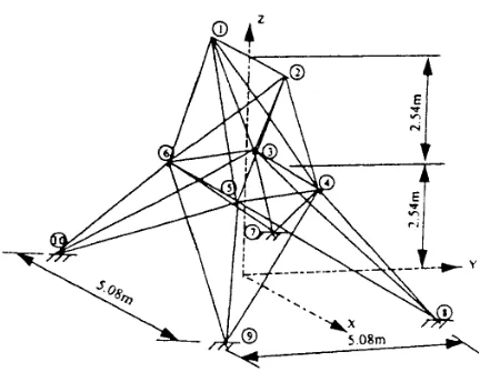
Figure 2. 25-bar space truss.
approximation methods are presented in Tables 1 and 2 for continuous and discrete optimization, respectively. In these tables the weight of the structure is given in Kg. Iteration number 0 indicates the initial design point. The optimal continuous and discrete design variables are given in Tables 3 and 4, respectively. Comparison of the methods in terms of the number of analyses, weight, execution time (wall-clock time) and maximum constraints for continuous optimization is presented in Table 5. From the numerical results, it can be seen that the number of required iterations in the proposed method is less than other methods. The execution time in all the methods is near, however, this is a small structure and the time can not be considered as a major factor.
7.2. Problem 2. 25-Bar Space Truss
The structure is shown in Figure 2 and the material properties are given as Young’s modulus, E = 6.9×10¹⁰ N/m2, weight density, ρ = 2.77×10³ Kg/m3 and allowable stresses, σt = + 2.76×10⁸ N/m2 for all tensile members [17]. Compression
stress limits and linking variables are given in Table 6. The structure is subjected to two load cases as shown in Table 7. The displacement limit TABLE 4. Optimum Design for 10-bar Truss (Discrete): cm2.
Member LA QA HLA HQA
1 180 180 180 190 2 15 1 5 10 3 165 155 155 160
4 85 85 100 90
5 10 5 5 5
6 0.645 5 1 0.645
7 75 70 55 60 8 115 140 140 130 9 115 135 135 130 10 20 5 5 10
TABLE 5. Comparison of the Results for 10-bar Truss.
No. conti. anal. No. discr. anal. Cont./discr. Weig. Execution time (sec.) Max. constraint
LA 9 5 2315/2317 4.0 0.066
QA 8 5 2294/2344 6.0 0.003
HLA 9 5 2286/2328 6.0 0.026
is ±8.89×10⁻³ m. the initial value and minimum size limits are 6.45×10⁻³ m2 and 6.45×10⁻⁵ m2, respectively. The set of available discrete values for the cross-sectional areas is
{
0.645, 1, 2, 3, 4, 5, ...}
(cm )Ai∈ 2
The results of this problem are given in Tables
8-12. In both continuous and discrete optimization, the number of required analyses in the present method is less than other methods.
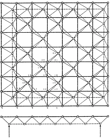
7.3. Problem 3. 132-Bar Grid Dome
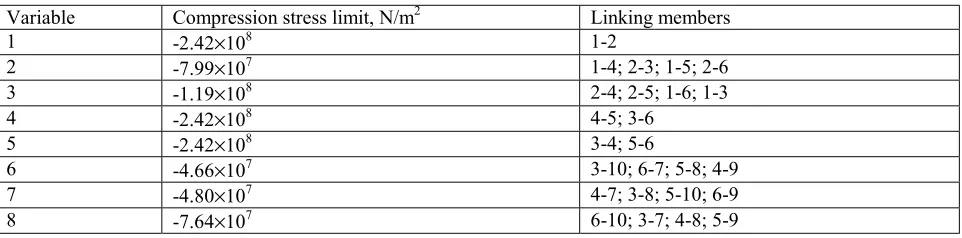
The 132 bar grid dome shown in Figure 3 chosen from Reference 16 is designed to support four independent load conditions and subjected to stress TABLE 6. Variable Linking and Allowable Stresses for 25-bar Truss.Variable Compression stress limit, N/m2 Linking members
1 -2.42×10⁸ 1-2
2 -7.99×10⁷ 1-4; 2-3; 1-5; 2-6
3 -1.19×10⁸ 2-4; 2-5; 1-6; 1-3
4 -2.42×10⁸ 4-5; 3-6
5 -2.42×10⁸ 3-4; 5-6
6 -4.66×10⁷ 3-10; 6-7; 5-8; 4-9
7 -4.80×10⁷ 4-7; 3-8; 5-10; 6-9
8 -7.64×10⁷ 6-10; 3-7; 4-8; 5-9
TABLE 7. Load Condition for 25-bar Truss (N).
Load case Joint X dir. Y dir. Z dir.
1 1 4450 44500 -22250
2 0 44500 -22250
3 2225 0 0
6 2225 0 0
2 5 0 89000 -22250
6 0 -89000 -22250
TABLE 8. Iteration Histories of 25-bar Truss for Continuous Variables.
Iteration No. LA QA HLA HQA
0 1500 1500 1500 1500
1 951 951 951 951 2 309 459 278 493 3 270 318 267 270 4 261 235 254 252 5 258 269 255 252 6 255 252 255
7 253 256
8 252 256
and displacements constraints. The allowable member stresses are taken as
1,4 j & 1,36 i , kg/cm 1723.75 σ
1723.75 ij 2 = =
− p p
where the subscripts i and j represent the member number and load condition, respectively. Minimum area constraints of 0.6452 cm2 are imposed on all members and displacement constraints of ±0.254 cm are prescribed at all joints in each coordinate direction. The structure is supported at all exterior joints. Young’s modules is taken as, 6.895 ×10⁵ Kg/cm2 and the material density as, 0.002768
Kg/cm3 for all members. Loads of 444.8 Kg are applied in the negative Z-direction for four independent load conditions given in Table 13. An initial area of 6.452 cm2 is prescribed for all members.
The structure is assumed to be symmetric about a vertical plane through joints 1, 40 and 52 and about a vertical plane through joints 1, 46 and 58. Thus the problem has 36 independent design variables, which are the areas of the members, Ai. All the design variables are allowed to take the following discrete values:
{
1, 2, 3, 4, 5,...}
(cm )Ai∈ 2
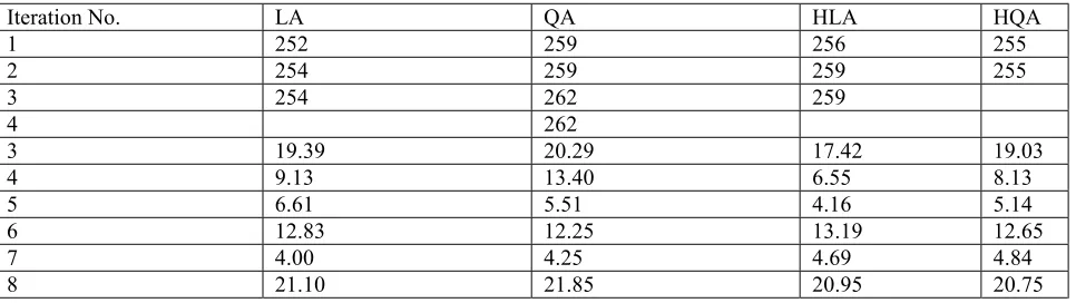
TABLE 9. Iteration Histories of 25-bar Truss for Discrete Variables.
Iteration No. LA QA HLA HQA
1 252 259 256 255
2 254 259 259 255
3 254 262 259
4 262
3 19.39 20.29 17.42 19.03
4 9.13 13.40 6.55 8.13
5 6.61 5.51 4.16 5.14
6 12.83 12.25 13.19 12.65
7 4.00 4.25 4.69 4.84
8 21.10 21.85 20.95 20.75
TABLE 10. Optimum Design for 25-bar Truss (Continuous): cm2.
Variable LA QA HLA HQA
1 0.645 2.04 0.712 12.20
2 3.37 2.34 5.86 2.22
TABLE 11. Optimum Design for 25-bar Truss (Discrete): cm2.
Variable LA QA HLA HQA
1 0.645 2 0.645 12
The continuous optimization is achieved with five analyses of the structure. One extra analysis is required to complete the discrete solution. The results are presented in Tables 14-18. For comparison, the problem is also solved by LA, QA and HLA methods. The performance of the present approach in both continuous and discrete optimization is better than other techniques. However, the execution time in LA and HLA is less, indicating that in this problem, the time required by the analysis is not significant.
7.4. Problem 4. Double-Layer Grid
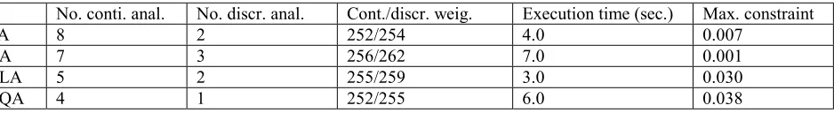
A double-layer grid of the type shown in Figure 4 with a span of 21 m and height of 1.5 m is chosen from Ref. [3]. The structure is simply supported at every other boundary joint of the bottom layer. TheTABLE 12. Comparison of the Results for 25-bar Truss.
No. conti. anal. No. discr. anal. Cont./discr. weig. Execution time (sec.) Max. constraint
LA 8 2 252/254 4.0 0.007
QA 7 3 256/262 7.0 0.001
HLA 5 2 255/259 3.0 0.030
HQA 4 1 252/255 6.0 0.038
TABLE 13. Load Condition for Dome.
Load cond. Loaded joints 1 1
2 1,2,3,4,7,8,9,10,11,12,13,19,20,21,22,23,24,25,26,27,28,37 3 All joints are loaded
4 1,4,5,6,7,13,14,15,16,17,18,19,28,29,30,31,32,33,34,35,36,37
TABLE 14. Iteration Histories of 132-bar Dome for Continuous Variables.
Iteration No. LA QA HLA HQA
0 197.7 197.7 197.7 197.7
1 203.3 200.3 203.2 200.3
2 104.5 181.6 57.56 152.5
3 86.23 87.35 75.38 96.35
4 83.33 85.01 80.41 80.13
5 82.56 86.68 84.10 79.76
6 83.47 84.62 83.64 79.79
7 79.97 84.68 81.53 79.76
8 78.93 84.55 81.53 79.77
9 78.93 84.55 81.53 79.77
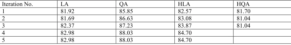
loading is assumed a uniformly distributed load on the top layer of intensity of 155.5 Kg/m2 and it is TABLE 15. Iteration Histories of 132-bar Dome for Discrete Variables.
Iteration No. LA QA HLA HQA
1 81.92 85.85 82.57 81.70
2 81.69 86.63 83.08 81.04
3 82.37 87.23 83.87 81.04
4 82.98 88.03 84.70
5 82.98 88.03 84.70
TABLE 16. Optimum Design for 132-bar Dome (Continuous): cm2.
Var. Member LA QA HLA HQA
1 3 6.44 6.70 5.97 5.58
2 4 6.42 5.59 6.53 6.96
3 9 5.66 5.57 5.40 5.37
4 10 5.61 6.90 5.25 5.61
5 19 2.43 4.95 3.62 2.36
6 20 3.06 2.86 3.19 3.47
7 21 2.83 3.55 3.02 2.96
8 22 3.41 3.21 3.25 3.43
9 23 3.14 3.00 3.31 3.33
10 35 2.56 2.85 2.59 2.68
11 36 2.82 3.26 2.82 2.90
12 37 2.55 2.74 2.70 2.58
13 53 2.08 3.78 3.20 2.44
14 54 2.30 1.68 1.85 1.97
15 55 2.56 2.75 2.83 2.92
16 56 2.80 2.19 2.67 2.65
17 57 2.29 2.30 2.38 2.08
18 58 3.24 3.36 3.29 3.20
19 59 2.51 1.78 2.21 2.47
20 60 3.01 3.31 3.36 3.38
21 79 1.26 1.27 1.26 0.98
22 80 1.08 1.20 1.15 1.62
23 81 1.62 1.74 1.56 1.60
24 82 1.11 1.08 1.10 0.91
25 83 0.698 5.14 3.36 1.00
26 105 1.92 2.07 2.17 2.45
27 106 1.35 1.02 0.862 0.99
28 107 2.41 2.67 2.52 2.71
29 108 2.67 2.63 2.99 2.41
30 109 1.90 2.40 2.28 1.98
31 110 2.93 2.74 2.46 2.72
32 111 1.51 1.37 1.51 1.70
33 112 0.835 1.39 0.658 0.669
34 113 2.16 2.40 2.38 2.12
35 114 2.29 2.12 2.16 2.01
transmitted to the joints acting as concentrated vertical loads only. The structure is assumed pin TABLE 17. Optimum Design for 132-bar Dome (Discrete): cm2.
Var. Member LA QA HLA HQA
1 3 6 7 6 6
2 4 6 6 7 7
3 9 6 6 5 5
4 10 6 7 5 6
5 19 2 5 4 2
6 20 3 3 3 3
7 21 3 4 3 3
8 22 3 3 3 3
9 23 3 3 3 3
10 35 3 3 3 3
11 36 3 3 3 3
12 37 3 3 3 3
13 53 2 4 3 2
14 54 2 2 2 2
15 55 3 3 3 3
16 56 3 2 3 3
17 57 2 3 2 2
18 58 3 3 3 3
19 59 3 2 2 2
20 60 3 3 3 3
21 79 1 1 2 1
22 80 1 2 2 2
23 81 2 2 2 2
24 82 2 1 2 1
25 83 1 5 3 1
26 105 2 2 2 2
27 106 2 1 1 1
28 107 3 3 3 3
29 108 3 3 3 2
30 109 2 2 2 2
31 110 3 3 2 3
32 111 2 2 2 2
33 112 1 2 2 1
34 113 2 3 2 2
35 114 3 2 2 2
36 115 2 3 3 4
TABLE 18. Comparison of the results for 132-bar dome.
No. con. No. dis. Con./discr. weig. Execution time (sec.) Max. constraint
LA 8 4 78.9/82.9 45.0 0.000001
QA 6 4 84.6/88.0 80.0 0.00033
HLA 7 4 81.5/84.7 40.0 0.00014
jointed with Young’s modules, 2.1 ×10⁶ Kg/cm2 and material density, 0.008 Kg/cm3 for all members. Member areas are linked to maintain symmetry about the four lines of symmetry in the plane of the grid. Thus the problem has 47 design variables. The initial areas are considered 20 cm2 with a lower limit of 0.1 cm2. The available
discrete values are
{
0.1, 0.3, 0.5, 1, 2, 3, 4, 5,...}
(cm )Ai∈ 2
Stress, Euler buckling and displacement constraints are considered in this problem. All the elements are subjected to the following stress constraints:
1,47 i , kg/cm 400 1 σ 000
1 i 2 =
− p p
where i is the element number. Tubular members are considered with a diameter to thickness ratio of 10. Thus Euler buckling is considered as
1,47 i , /8L 10.1EA σ
σi ≥ bi =− i 2i =
where Ai and Li are the cross-sectional area and length of the ith element, respectively.
In addition, displacement constraints are imposed on the vertical component of the three central joints along the diagonal of the grid (joints 19, 20 and 22) as
1,2,3 i 1.5cm, δ
1.5cm≤ i ≤ =
−
The results are presented in Tables 19-23. The efficiency of HQA method in terms of the number of iterations is better than other approaches. In all the problems under investigation, it was noticed that this method is very stable and the changes in the parameters such as multipliers r and s do not influence the convergence process. In some methods like LA, sometimes difficulties arise for problems to converge and changing Figure 4. Double layer grid
TABLE 19. Iteration Histories of Double Layer Grid for Continuous Variables.
Iteration LA QA HLA HQA
0 3781.0 3781.0 3781.0 3781.0
1 3650.6 3650.6 3405.9 3650.6
2 1377.3 3015.4 1177.0 2964.5
3 1210.2 1218.4 1136.5 1360.2
4 1144.8 1201.6 1134.2 1092.6
5 1142.8 1147.1 1132.6 1056.0
6 1138.8 1136.4 1124.7 1056.1
7 1128.8 1136.4 1106.9 1056.1
8 1128.8 1106.9
TABLE 20. Iteration Histories of Double Layer Grid for Discrete Variables.
Iteration LA QA HLA HQA
1 1131.9 1144.6 1127.1 1060.5
2 1132.4 1147.6 1122.0 1060.5
3 1134.2 1150.7 1117.5
4 1134.7 1154.6 1117.5
5 1139.3 1154.6
6 1141.5
move limits, initial design point and other optimization parameters is necessary to get a proper convergence.
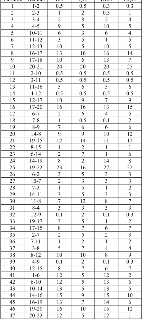
For the size of problems considered in this study, the computational time of QHA is slightly larger than other methods. For these problems this TABLE 22. Optimum Design for double layer grid (discrete): cm2.
Variable Member LA QA HLA HQA
1 1-2 0.5 0.5 0.3 0.3 2 2-3 1 2 0.3 1 3 3-4 2 8 2 4 4 4-5 9 5 10 5
5 10-11 6 3 6 4
6 11-12 3 5 1 5
7 12-13 10 5 10 5
8 16-17 13 16 16 14
9 17-18 10 6 13 7
10 20-21 24 20 20 25
11 2-10 0.5 0.5 0.5 0.5 12 3-11 0.5 0.5 0.5 0.5
13 11-16 5 6 5 6
14 4-12 0.5 0.5 0.5 0.5
15 12-17 10 9 7 9
16 17-20 16 16 13 15
17 6-7 2 6 4 5
18 7-8 1 0.5 0.1 2
19 8-9 7 6 6 6
20 14-8 9 9 10 12
21 19-15 12 14 11 12
22 8-15 1 2 1 1
23 6-14 2 7 1 6
24 14-19 8 2 14 8
25 19-22 23 16 27 22
26 6-2 3 5 3 3
27 10-7 2 3 3 3
28 7-3 1 5 1 2
29 14-11 3 5 3 3
30 11-8 7 13 8 7
31 8-4 3 3 3 3
32 12-9 0.1 2 0.1 0.3
33 19-17 3 5 1 2
34 17-15 8 7 6 7
35 2-7 2 5 2 3
36 7-11 1 2 1 2
37 3-8 5 7 4 4
38 8-12 10 10 8 9 39 4-9 0.1 2 0.1 0.3
40 12-15 8 7 6 7
41 1-6 12 5 12 2
42 6-10 12 5 13 6
43 10-14 13 5 13 5
44 14-16 15 9 15 10
45 16-19 13 7 14 6
46 19-20 16 10 15 12
47 20-22 12 5 12 1
TABLE 21. Optimum Design for Double Layer Grid (Continuous): cm2.
Variable Member LA QA HLA HQA
1 1-2 0.42 0.42 0.27 0.27 2 2-3 0.59 1.97 0.20 1.34 3 3-4 1.65 8.31 2.31 4.06 4 4-5 8.61 5.45 9.74 4.49 5 10-11 4.54 3.09 5.87 3.95 6 11-12 3.05 5.31 0.92 4.59 7 12-13 9.69 5.12 10.32 5.39 8 16-17 12.95 16.01 16.28 13.56 9 17-18 10.14 5.55 13.10 7.27 10 20-21 23.76 19.73 20.18 24.93 11 2-10 0.51 0.50 0.50 0.50 12 3-11 0.50 0.50 0.50 0.54 13 11-16 4.87 5.69 5.19 5.97 14 4-12 0.52 0.5 0.50 0.56 15 12-17 10.01 9.09 7.16 8.76 16 17-20 16.00 15.85 12.67 15.23 17 6-7 1.93 5.51 3.57 5.42 18 7-8 0.97 0.40 0.14 2.01 19 8-9 7.03 5.84 6.23 5.62
20 14-8 9.31 9.02 9.63 12.21
21 19-15 11.96 13.63 11.02 11.98 22 8-15 0.86 1.78 1.03 0.93 23 6-14 2.36 6.95 9.50 5.71 24 14-19 7.65 2.24 13.62 8.06 25 19-22 23.29 16.11 26.97 22.06 26 6-2 3.28 4.50 3.14 3.24 27 10-7 2.31 2.44 2.69 2.79 28 7-3 0.62 4.80 1.01 1.74 29 14-11 3.29 4.69 2.81 3.22
30 11-8 6.64 12.72 7.64 7.40
31 8-4 3.20 3.14 3.23 3.13 32 12-9 0.101 1.64 0.14 0.22 33 19-17 2.63 3.58 1.18 2.16 34 17-15 8.00 7.25 5.61 6.66 35 2-7 1.49 4.99 1.74 2.57 36 7-11 0.97 2.20 1.48 1.86 37 3-8 4.72 6.70 3.57 3.90 38 8-12 10.16 9.49 7.70 9.31 39 4-9 0.12 1.64 0.14 0.21 40 12-15 8.12 7.29 5.61 6.58 41 1-6 12.34 5.41 11.72 2.22 42 6-10 12.30 5.39 12.81 5.62 43 10-14 12.84 5.19 12.82 4.84
44 14-16 14.64 8.88 15.27 10.21
is reasonable as the time taken by the optimization process is greater than the time required by the analysis. The overall computational time to achieve an optimal solution depends on the number of design variables, number of constraints and the size of the problem in terms of the degrees of freedom. Usually, all the constraints are not considered in each design iteration and some of the critical or near critical constraints are retained. The number of retained constraints is two to three times the number of design variables. Thus only the number of variables and the number of degrees of freedom has a great influence on the computational time. Practical design problems have 10 to 50 variables and several thousand degrees of freedom. In such cases, the cost of analysis dominates the overall cost. Therefore, in large-scale problems, reducing the number of iterations has an important role on the overall computational cost of optimization.
8. CONCLUSIONS
An efficient second order hybrid approximation is presented for the functions that are required in the process of continuous and discrete optimization. The exact evaluation of these functions is computationally expensive, thus the introduction of the approximate functions creates a robust optimization process. First the continuous optimization is obtained by a penalty function, then the discrete variables are obtained by presenting a new penalty function with the use of the same approximation concepts. The main features of the proposed technique are that the second order derivatives are established by the available first order derivatives. In addition, only the diagonal elements of the Hessian matrix are estimated. The
numerical results indicate that with this form of simplification, a high quality approximation is established. Also the hybrid second order approximation is stable to converge and parameters such as penalty function multipliers, initial point and move limits do not change the convergence process. In this method for small size problems, the execution time is slightly higher, however, for large structures in terms of the number of degrees of freedom, the overall computational cost would decrease.
9. REFERENCES
1. Schmit, L. A. Jr., and Farshi, B, “Some Approximation Concepts for Structural Synthesis”, AIAA Journal, Vol. 12, No. 5, (1974), 692-699.
2. Mills-Curran, W. C., Lust, R. V., and Schmit, L. A. Jr., “Approximation Methods for Space Frame Synthesis”, AIAA Journal, Vol. 21, No. 11, (1983), 1571-1580. 3. Salajegheh, E. and Vanderplaats, G. N., “An Efficient
Approximation Method for Structural Synthesis with Reference to Space Structures”, Int. J. Space Structures, Vol. 2, (1986/1987), 165-175.
4. Wang, L. and Grandhi, R. V., “Recent Multi-Point Approximation in Structural Configuration”, in: WCSMO-1 (ed. N. Olhoff and G.I.N. Rozvany), Proc. F i r s t W o r l d C o n g r e s s o f S t r u c t u r a l a n d Multidisciplinary Optimization, Oxford, Pergamon, (1995), 75-82.
5. Salajegheh, E., “Optimum Design of Plate Structures Using Three Point Approximation”, Structural Optimization, Vol. 13, No. 2/3, (1997), 140-147. 6. Salajegheh, E. and Rahmani, A., “Optimum Shape
Design of Three Dimensional Continuum Structures Using Two Point Quadratic Approximation”, in: Advances in Computational Structural Mechanics (ed. B.H.V. Topping), Proc. Fourth Int. Conf. on Computational Structures Technology, Edinburgh, Civil-Comp Press, (1998), 435-439.
7. Barthelemy, J. F. M. and Haftka, R. T., “Approximation Concepts for Structural Design-a Review”, Structural Optimization, Vol. 5, (1993), 129-144.
TABLE 23. Comparison of the Results for Double Layer Grid.
No. con. No. Dis. Conti./Discr. weight Execution time (sec.) Max. constra.
LA 7 6 1128.8/1141.5 30.0 0.061
QA 6 4 1136.4/1154.6 105.0 0.087
HLA 7 3 1106.9/1117.5 30.0 0.086
8. Arora, J. S., Huang, M. W., and Hsieh, C.C., “Methods for Optimization of Nonlinear Problems with Discrete Variables: a Review”, Structural Optimization, Vol. 8, (1994), 69-85.
9. Shin, D. K., Gurdal, Z. and Griffin, O. H. Jr., “A Penalty Approach for Nonlinear Optimization with Discrete Design Variables”, Engineering Optimization, Vol. 16, (1990), 29-42.
10. Cai, J. and Thierauf, G., “Discrete Optimization of Structures Using an Improved Penalty Function Method”, Engineering Optimization, Vol. 21, (1993), 293-306.
11. Salajegheh, E., “Discrete Variable Optimization of Plate Structures Using Penalty Approaches and Approximation Concepts”, Engineering Optimization, Vol. 26, (1996), 195-205.
12. Salajegheh, E. “Approximate Discrete Optimization of Frame Structures with Duel Methods”, Int. J. for Numerical Methods in Engineering, Vol. 39, No. 9,
(1996), 1607-1617.
13. Salajegheh, E., “Discrete Variable Optimization of Plate Structures Using Dual Methods”, Computers and Structures, Vol. 58, No. 6, (1996), 1131-1138.
14. Haftka, R. T. and Starnes, J. H. Jr., “Application of a Quadratic Extended Interior Penalty Function in Structural Optimization”, AIAA Journal, Vol. 14, No. 6, (1976), 718-724.
15. Starnes, J.H. Jr., and Haftka, R.T., “Preliminary Design of Composite Wings for Buckling, Stress and Displacement Constraints”, Journal of Aircraft, Vol. 16, (1979), 564-570.
16. Salajegheh, E. and Vanderplaats, G. N., “Efficient Optimum Design of Structures with Discrete Design Variables”, Int. J. Space Structures, Vol. 8, No. 3, (1993), 199-208.