SIMULATION OF STYRENE POLYMERIZATION IN
ARBITRARY CROSS-SECTIONAL DUCT REACTORS
BY BOUNDARY-FITTED COORDINATE
TRANSFORMATION METHOD
M. A. Isazadeh
Department of Chemical Engineering, University of Petroleum Industry Ahwaz, Iran
(Received: February 19, 2000 - Accepted in Final From: October 21, 2001)
Abstract The non-orthogonal boundary-fitted coordinate transformation method is applied to the solution of steady three-dimensional conservation equations of mass, momentum, energy and species-continuity to obtain the laminar velocity, temperature and concentration fields for simulation of polymerization of styrene in arbitrary cross-sectional duct reactors. Variable physical properties (except for specific-heat), viscous heat dissipation and free-convection effects are considered in modeling while axial diffusion is ignored. The conservation equations originally written in Cartesian coordinates are parabolized in the axial direction and then transformed to the non-orthogonal curvilinear coordinates to handle arbitrary duct geometries. The transformed equations are discretized by the control-volume finite-difference approach in which the convective and diffusive terms are handled by the upwind-difference and central-difference approximation schemes respectively. Results are obtained for eight different geometries. The results show that not a specific geometry is in general superior to conventional circular duct reactors for the highest conversion of the chemical reaction under study, considering also the least pressure-drop in the reactors.
Keywords Boundary-Fitted Coordinate, Styrene Polymerization, Arbitrary Cross-Sectional Duct Reactors
ﻩﺪﻴﻜﭼ
ﻩﺪﻴﻜﭼ
ﻩﺪﻴﻜﭼ
ﻩﺪﻴﻜﭼ
ﻪﺳﺖﺧﺍﻮﻨﻜﻳﺕﻻﺩﺎﻌﻣﻞﺣﻱﺍﺮﺑﻲﺳﺪﻨﻫﺎﻜﺷﺍﺩﻭﺪﺣ ﻩﺪﻧﺮﻴﮔﺮﺑﺭﺩﺕﺎﺼﺘﺨﻣ ﻝﺎﻘﺘﻧﺍﺪﻣﺎﻌﺘﻣﺮﻴﻏ ﺵﻭﺭ
،ﻢﺘﻨﻣﻮﻣ،ﻡﺮﺟﺀﺎﻘﺑﻱﺪﻌﺑ ﻭﻱﮊﺮﻧﺍ
ﺍﻡﻭﺍﺪﺗ ﺍﺰﺟ ﻭﺎﻣﺩﻊﻳﺯﻮﺗﺰﻴﻧﻭﻡﺍﺭﺁﻥﺎﻳﺮﺟﺭﺩﺖﻋﺮﺳﻊﻳﺯﻮﺗﺎﺗﻩﺪﺷﻩﺩﺮﺑﺭﻝﺎﻜﺑ
ﭘ ﻱﺯﺎﺳ ﻪﺑﺎﺸﻣ ﻱﺍﺮﺑ ﺖﻈﻠﻏ ﻠ
ﺪﻳﺁﺖﺳﺪﺑ ﻩﺍﻮﺨﻟﺩﻊﻄﻘﻣ ﺡﻮﻄﺳ ﺎﺑ ﻱﺎﻫﺭﻮﺘﻛﺍﺭ ﺭﺩﻦﻳﺮﻳﺎﺘﺳﺍ ﻥﻮﻴﺳﺍﺰﻳﺮﻤﻴ
.
ﺹﺍﻮﺧ
ﺮﻴﻐﺘﻣﻲﻜﻳﺰﻴﻓ
)
ﺮﻴﻏ
ﻩﮋﻳﻭﻱﺎﻣﺮﮔﺯﺍ
(
ﻛﺕﺍﺮﺛﺍﻭﻱﮊﺮﻧﺍﻲﮕﺘﻓﺭﺭﺪﻫ، ﻨ
ﺮﻈﻧﺭﺩﻱﺰﻳﺭﻝﺪﻣﺭﺩﺩﺍﺯﺁﻥﻮﻴﺴﻛﻮ ﻪﺘﻓﺮﮔ
ﻩﺪﺷ
؛ٍ ﻟﺎﺣﺭﺩ ﻴ
ﺯﺍﻪﻜ ﺫﻮﻔﻧ
ﺖﺳﺍﻩﺪﺷﺮﻈﻨﻓﺮﺻﻱﺭﻮﺤﻣ
. ﻩﺪﺷﻪﺘﺷﻮﻧﻦﻳﺰﺗﺭﺎﻛﺕﺎﺼﺘﺨﻣﺭﺩﺍﺪﺘﺑﺍﺭﺩﻪﻛﺀﺎﻘﺑﺕﻻﺩﺎﻌﻣ
ﻲﻨﺤﻨﻣﺪﻣﺎﻌﺘﻣﺮﻴﻏﺕﺎﺼﺘﺨﻣﻢﺘﺴﻴﺳﻪﺑﺲﭙﺳﻭﻩﺪﺷﻩﺰﻴﻠﺑﺍﺭﺎﭘﻱﺭﻮﺤﻣﺖﻬﺟﺭﺩ
-ﻝﺎﻘﺘﻧﺍﻲﻄﺧ
ﻝﺎﻜﺷﺍﺎﺗﺪﻨﺑﺎﻳﻲﻣ
ﺪﻧﺮﻴﮔﺮﺑﺭﺩﺍﺭﻩﺍﻮﺨﻟﺩﻲﺳﺪﻨﻫ
. ﺎﺑﻪﺘﻓﺎﻳﻝﺎﻘﺘﻧﺍﺕﻻﺩﺎﻌﻣ ﻮﻴﺷ
ﻩ
،ﻲﻫﺎﻨﺘﻣ ﺕﻼﺿﺎﻔﺗﺵﻭﺭﺭﺩﻲﻤﺠﺣﻝﺮﺘﻨﻛ ﻳﺯﻮﺗ
ﻲﻌ
ﻪﺘﻓﺎﻳﻪﺘﺴﺴﮔ ﻳﺭﻮﻄﺑ
ﻭﻥﻮﻴﺴﻛﻮﻨﻛﺕﻼﻤﺟ ﻪﺑﻥﺁﺭﺩﻪﻜ ﺫﻮﻔﻧ
ﺩﺭﻮﺧﺮﺑﺩﻮﺨﺑﺹﻮﺼﺨﻣﻱﺎﻫﺪﺘﻣﺎﺑ ﻲﻣ
ﺩﻮﺷ
.
ﺞﻳﺎﺘﻧ
ﻲﻣﻥﺎﺸﻧﻒﻠﺘﺨﻣﻲﺳﺪﻨﻫﻞﻜﺷﺖﺸﻫﻱﺍﺮﺑﻩﺪﻣﺁﺖﺳﺪﺑ
ﺪﻫﺩ
ﻪﻛ
ﻮﺼﺨﺑﻲﺳﺪﻨﻫﻞﻜﺷﭻﻴﻫ
ﻲﺻ
ﻲﻠﻛﺖﻟﺎﺣﺭﺩ
ﺮﻳﺍﺩﻊﻄﻘﻣﺡﻮﻄﺳﺎﺑﻱﺎﻫﺭﻮﺘﻛﺍﺭﺮﺑ ﻱﺍﻩ
ﺍ
ﺭﺍﺪﻘﻣﻦﻳﺮﺘﺸﻴﺑﺮﻈﻧﺯ
ﻞﻳﺪﺒﺗ
ﺎﻴﻤﻴﺷﺶﻨﻛﺍﻭﺭﺩ ﻳ
ﻞﻗﺍﺪﺣﻭﻪﻌﻟﺎﻄﻣﺩﺭﻮﻣﻲ
ﺭﻮﺘﻛﺍﺭﺭﺩﺭﺎﺸﻓﺖﻓﺍ ،
ﺩﺭﺍﺪﻧﺯﺎﻴﺘﻣﺍ
.
INTRODUCTION
The purpose of this paper is to provide simultaneous heat and mass transfer solution of steady laminar flow polymerization of styrene in arbitrary cross-sectional duct reactors.
A review of literature in this area reveals that the previous investigations carried-out for simulation of polymerization of styrene are only in conventional cylindrical reactors. Sala et al. [1] analyzed styrene polymerization by solving the steady, two dimensional conservation equations
isothermal tubular reactors was analyzed. It was concluded that adequate control of the polymerization can he achieved by maintaining the tube wall temperature below the inlet feed temperature to inhibit thermal runaway.
Wyman et al. [2] introduced an approximate model to calculate the number and weight-average molecular weights of the polymer being produced in a continuous steady-state tubular reactor from the zeroth, first and second moments of radical and polymer distributions. The partial differential equations describing temperature, velocity and composition were written considering axial symmetry and incompressible laminar flow in a cylindrical tube allowing for variable viscosity amid conductivity. The reaction rate constant was of Arrhenius type in which the so-called gel effect was also taken into account. The pressure drop in the tube was obtained from the equation of motion. Radial convection, axial conduction and viscous heating of polymer in the energy balance equation were neglected. The radial and angular components of velocity were ignored in the equation of motion. The partial differential equations were solved numerically using the classical explicit finite-difference method.
Husain et al. [3] made a computational study of bulk thermal polymerization of styrene in a tubular reactor in which the fluid rheology was represented by a power-law model. They considered the polymer to be a non-diffusing specie and neglected radial velocities. They also neglected the axial diffusion of mass and energy. They took into account the gel effect following Hui et al [4]. Finite differencing radially and solving the resulting equations using a fourth-order Runge-Kutta-Gill routine solved the system of differential equations.
Valsamis et al. [5,6] used piston flow and segregated flow models for the polymerization of styrene in tubular reactors. Experiments were performed in a helically coiled tube with a length of 14.6 m and a diameter of 0.46 cm. Running pure thermal styrene polymerization at 160 degrees Celsius yielded a conversion of 15% in 5.15 minutes residence time.
Chen et al [7,8] determined the residence time washout function theoretically by means of flow models and experimentally by inert tracer techniques. Introducing steady mass, momentum and energy transport equations for laminar axisymmetric flow in cylindrical coordinates using fully developed
The objective of this study is to employ a numerical solution method [11] based on non-orthogonal boundary-fitted coordinate transformation and make any developments required to apply to the simulation of polymerization of styrene in complex geometry cross-sectional duct reactors. Results are obtained for eight different geometries and for five different sets of operating conditions.
THE MATHEMAT ICAL MODELLING
The strongly conservative form [12] of the steady overall continuity, momentum energy and species continuity equations are expressed as follows:
The Overall Continuity Equation
0) v .
(∇ρ = (1)
The Momentum Equation
0 g ) . ( P ) vv .(∇ρ −∇ − ∇τ +ρ =
− (2)
The Energy Equation
0 Q ) v : ( ) q . ( ) Tv C .
(∇ρ P − ∇ − τ ∇ + R=
− (3)
The Reactant Continuity Equation
A A A
Av) ( . D m ) R m
.
(∇ρ = ∇ρ ∇ − (4) The coordinate axes selected for the Cartesian domains are shown in Figure 1.
The Constitutive Equation
The rheological behavior of polystyrene can be adequately expressed by power-law non-Newtonian model [3,9,10]. For power-law model the stress-tensor is related to the rate-of-strain tensor [13] by the following relationship: ij 1 n ij ijij ( :
2 1 ∆ ∆ ∆ µ − = τ − (5)
The Parabolized Governing Equations in
Cartesian Coordinates
The overall continuity equation 0 ) pw ( z ) v ( y ) u (x ∂ =
∂ + ρ ∂ ∂ + ρ ∂ ∂ (6)
The Momentum Equations
x-Component ) y x ( x P ) wu ( z ) vu ( y ) u ( x yx xx 2 ∂ τ ∂ + ∂ τ ∂ − ∂ ∂ − = ρ ∂ ∂ + ρ ∂ ∂ + ρ ∂ ∂ (7) y-Component g ) ( ) y x ( y P ) pwv ( z ) pv ( y ) puv ( x a yy xy 2 ρ − ρ − ∂ τ ∂ + ∂ τ ∂ − ∂ ∂ − = ∂ ∂ + ∂ ∂ + ∂ ∂ (8) z-Component
)
y
x
(
dz
P
d
)
pw
(
z
)
pvw
(
y
)
uw
(
x
yz xz 2∂
τ
∂
+
∂
τ
∂
−
−
=
∂
∂
+
∂
∂
+
ρ
∂
∂
−(9)
The Energy Equation
A v P P P R ) H ( . M ) y T k ( y ) x T k ( x ) Tw C ( z ) Tv C ( y ) Tu C ( x ∆ − + Φ + ∂ ∂ ∂ ∂ + ∂ ∂ ∂ ∂ = ρ ∂ ∂ + ρ ∂ ∂ + ρ ∂ ∂ (10)
The Reactant Continuity Equation
A A A A A A A A R ) y m D ( y ) x m D ( x ) w m ( z ) v m ( y ) u m ( x − ∂ ∂ ρ ∂ ∂ + ∂ ∂ ρ ∂ ∂ = ρ ∂ ∂ + ρ ∂ ∂ + ρ ∂ ∂ (11)
buoyancy term in the “y” momentum equation. In cases of negligible buoyancy effect, P would be the total pressure defined as hydrostatic plus dynamic pressures. The term M is the apparent viscosity for the power-law non-Newtonian fluid.
The Boundary Conditions
Inlet (@z=0) Axial Velocity A uniform entrance
velocity profile is specified at inlet: inlet
w
w= (12)
Transverse Velocities It is assumed that there is
no secondary flow at inlet: 0
v , 0
u= = (13)
Temperature A uniform temperature-profile is
specified at inlet:
inlet
T
T
=
(14)Reactant Weight Fraction For an unconverted
reactant at inlet: 1
=
m (15)
Walls of the Duct
Axial Velocity No slip-condition is assumed on the walls of the duct:0
=
w (16)
Transverse Velocities 0 v , 0
u= = (17) Temperature For a constant wall- temperature:
wall T
T= (18)
Reactant Weight-Fraction The material does
not, move through the wall: 0 n m = ∂ ∂ (19)
Outflow Condition (©z = L) For the
parabolized governing equations used here no
downstream boundary conditions are required.
THE BOUNDARY-FITTED METHOD
The development of the boundary-fitted coordinate systems brought about the coordinate transformation of the physical domain, such as Cartesian coordinates
to the curvilinear coordinates so that all the boundaries match the coordinate lines in the new system and the need to interpolate the boundary conditions as practiced before is eliminated [14,15].
The curvilinear coordinate system may be either orthogonal or non-orthogonal in the sense of the mesh generated over the physical-domain. In this study the non-orthogonal method is applied to obtain solutions of the present three-dimensional problem in irregular cross-sectional ducts.
TRANSFORMATION OF GOVERNING PDE’S
It is necessary to transform the partial-differential equations under consideration into the new coordinate variables before being discretized. In general, the transformation operation generates additional terms in the governing equations so that these equations become more complicated upon transformation. The physical Cartesian velocities are retained as the dependent variables in transformation. However, the contra-variant velocity components also take part in the structure of the transformed equations. The transformed equations are as follows:
The Overall Continuity Equation
0 ) w ( ) V ( ) U
( ρ =
σ ∂ ∂ + ρ η ∂ ∂ + ρ ζ ∂ ∂ (20)
The Momentum Equations
z-Component
σ
−
τ
−
τ
η
∂
∂
−
τ
−
τ
ζ
∂
∂
−
=
σ
∂
∂
+
η
∂
∂
+
ρ
ζ
∂
∂
− ζ ζ η ηd
P
d
J
)]
ˆ
(
y
)
ˆ
(
[x
)]
ˆ
(
x
)
ˆ
(
y
[
)
pwW
(
)
pwV
(
)
wU
(
xz yz yz xzThe Energy Equation
A v P P P
Rˆ
)
H
(
J
ˆ
M
ˆ
J
kT
J
kT
J
kT
J
kT
J
)
TW
C
(
)
TV
C
(
)
TU
C
(
∆
−
+
Φ
+
β
−
γ
η
∂
∂
+
β
−
α
ζ
∂
∂
=
ρ
σ
∂
∂
+
ρ
η
∂
∂
+
ρ
ζ
∂
∂
ζ η η ζThe Reactant Continuity Equation
A ^ A A A A A A A
R
J
m
J
D
m
J
D
m
J
D
m
J
D
)
W
m
(
)
V
m
(
)
U
m
(
−
ρ
γ
−
ρ
β
η
∂
∂
+
ρ
α
−
ρ
β
ζ
∂
∂
=
ρ
σ
∂
∂
+
ρ
η
∂
∂
+
ρ
ζ
∂
∂
ζ η η ζwhere
m
=
m
A for derivatives.Boundary Conditions
Inlet (@σ =0)
(i) Axial Velocity w(ζ,η)=winlet (26)
(ii) Transverse Velocities
0
)
,
(
v
,
0
)
,
(
u
ζ
η
ζ
η
=
(27)
(iii) Temperature inlet T ) , (
T ζ η = (28)
(iv) Reactant Weight-Fraction
0
.
1
)
,
(
m
ζ
η
=
(29)Walls of the Duct
(i) Axial Velocity1 1
L
,
1
for
1
M
1
(
,
)
0
1
L
1
for
1
,
M
w
=
ζ
≤
η
≤
≤
ζ
≤
η
=
=
η
ζ
(30)
(ii) Transverse Velocities
1 1
L
,
1
for
1
M
1
M
,
1
for
1
L
1
0
)
,
(
v
0
)
,
(
u
=
ε
≤
η
≤
≤
ζ
≤
η
=
=
η
ζ
=
η
ζ
(31)
(iii) Temperature 1 1 wall L , 1 for 1 M 1( , ) T . 1 L1 for 1,M T
= ζ ≤
η
≤≤ζ≤ η=
= η
ζ
(32)
(iv) Reactant Weight-Fraction
Note that the transformation parameters are as follows
ξ η η ζ ζ ζ ζ ζ η ε η ζ η η
−
=
=
+
=
γ
=
+
=
−
β
α
=
+
=
−
y
x
y
x
J
x
y
W
Jw
u
y
v
x
V
y
y
x
x
v
x
u
y
U
y
x
2 2 η η 2 2 (33)DISCRETIZATION OF TRANSFORMED EQUATIONS
For a non-orthogonal grid system, the best grid configuration is a modified classical staggered-grid (Figure 2) in which both components of u and v velocities are used coincidentally at the same location with the contra-variant velocities normal and parallel to the faces of the cell [16].
The transformed governing equations are discretized using the method known as the control-volume approach [17,18]. The upwind difference scheme is used for discretization of convective terms and the central difference scheme is used for discretization of diffusion terms. The discretization equations are algebraic equations and are solved by a line-by-line tridiagonal matrix (TDMA) algorithm. For the proper location of the control-volume faces, the B-type grid is employed here [18]. The SIMPLER algorithm handles the pressure-velocity coupling in the transverse direction after being modified for the orthogonal coordinate system and non-Newtonian fluids. The method adopted in this work to handle the pressure-velocity coupling in (23)
(24)
(25)
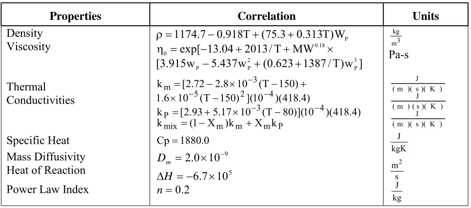
TABLE 1. Fluid Properties Data.
Properties Correlation
Units
Density
Viscosity
Thermal
Conductivities
Specific Heat
Mass Diffusivity
Heat of Reaction
Power Law Index
]
w
)
T
/
1387
623
.
0
(
w
437
.
5
w
915
.
3
[
MW
T
/
2013
04
.
13
exp[
W
)
T
313
.
0
3
.
75
(
T
918
.
0
7
.
1174
3 P 2 P P 18 . 0 0 P+
+
−
×
+
+
−
=
η
=
−
+
+
ρ
P m m m mix 4 3 P 4 2 5 3 m k X k ) X 1 (k [2.93 5.17 10 (T 80)](10 )(418.4) k ) 4 . 418 )( 10 ]( ) 150 T ( 10 6 . 1 ) 150 T ( 10 8 . 2 72 . 2 [ k + − = + × − = − × + − × − = − − − − − 0 . 1880 Cp= 9
10
0
.
2
×
−=
mD
510
7
.
6
×
−
=
∆
H
2 . 0 = n 3 m kgPa-s
) K )( s )( m (Js)( K ) ( ) m (
J)( K ) s )( m ( J kgK J kg J s m2
the axial direction is that of Raithby and Schneider [19].
RESULTS AND DISCUSSION
In this study the thermal polymerization of styrene is analyzed in noncircular cross-sectional duct reactors. The rate equation for this reaction [7-10], considering third-order thermal initiation is expressed by: 5 . 2 2 1 i 2 1 t P
P (2k ) (M) k k R
= (34)
in which ) s ( ) kg ( m e 10 019 . 2 k 2 6 ) T / 13810 ( 1
i = × − (35)
) s )( kg ( m e 10 009 . 1 k 3 ) T / 3557 ( 5
p = × − (36)
) s )( kg ( m e 10 218 . 2 k 3 ) T / 6377 ( 4 m ,
tr = × − (37)
) s )( kg ( m e e 10 205 . 1 k 3 )] w A w A w A ( 2 [ ) T / 844 ( 7 t 3 P 3 2 P 2 P
1 + + − − × = where
03
.
3
T
10
85
.
7
03
.
3
A
T
10
76
.
1
56
.
9
A
T
10
05
.
5
57
.
2
A
3 3 2 2 3 1−
×
+
−
=
=
−
×
×
−
=
− − − (39) The physical properties of the system are shown in Table1. The system model and computer codes are validated in the following section (i) to (iii). There exists a close agreement between the simulation results of the previous investigators and the present simulation study.The effect of free convection in this study is ignored for the results to he comparable with literature data in which this effect is not considered. Further investigations, which are presented in the following pages, show that conversion results are only negligibly affected if free convection is considered. The effect of variation of number of stations in the axial direction is in indicated for two cases, which show a. satisfactorily close agreement in the results of conversion.
Section (i)
Husain and Hamielec [3]: • length of tube: 500 cm• tube radius: 2.0 cm
• inlet velocity: 0.0695 cm/sec
• inlet/wall temperature: 1000C /1000C
The results obtained in the present analysis are as follows:
(for 5 stations selected in axial direction)
• conversion: 1.38 wt % (for 100 cm tube length)
• conversion: 4.14 wt % (for 300 cm tube length)
• conversion: 6.74 wt % (for 500 cm tube length) (for 10 stations selected in axial direction)
• conversion: 1.37 wt % (for 100 cm tube length)
• conversion: 3.95 wt % (for 300 cm tube length)
• conversion: 6.43 wt % (for 500 cm tube length) These results are in good agreement with the results of Husain and Hamielec [3] who validated their analysis by experimental data of Wallis [3], which included both chemically and thermally, initiated polymerization of styrene.
Section (ii)
Chi-Chi Chen [7]:• length of tube: 6.4 cm
• tube radius: 0.55 cm
• mass flow: 1.345x1O-4 kg/sec
• inlet/wall temperature: 1400C / 1350C
• conversion: 26.49 wt%.
The result obtained in the present study is 26.6 wt % conversion which is close to the result obtained above.
Section (iii) Kleinstreuer and Agarwal [9]: • length of tube: 5.0 m
• tube radius: 2 cm
• mass flow: 0.00002 kg/sec
• inlet /wall temperature: 1300C/1000C
• conversion: 54.8 wt %
• velocity profile: parabolic
The results obtained in the present study are 55.35 wt % and 55.22 wt % for parabolic and uniform velocity profiles respectively.
Following to the validation of the system modeling and computer code, the simultaneous flow, heat and mass transfer problem was solved for thermal polymerization reactors with different cross-sectional geometries, employing 5 sets of operating conditions indicated in Table 2.
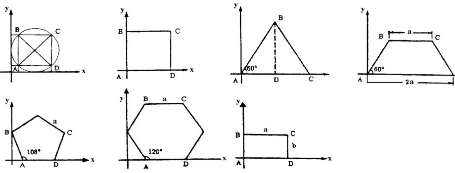
The selection of duct geometries of interest and even the angles and side-lengths of some of them is a matter with infinite choices. However, some standard geometries were selected as there was no preference to choose a specific one. These configurations are as follows:
• circular duct,
• square duct,
• equilateral triangular duct,
• trapezoidal duct (acute angle =600, one side twice the other),
• pentagonal duct (each angle = 1080)
• hexagonal duct (each angle = 1200)
• rectangular duct (aspect ratio 1.5)
• rectangular duct (aspect ratio: 2.0) These geometries are shown in Figure 3.
For the sake of numerical accuracy and computational economy a 21x21 grid was selected in transverse direction. The CPU time was about 10 minutes for one run on IBM ESA9000 machine. About 5 iterations were required
TABLE 2. Operating Conditions.
Case Winlet
(m/s)
T inlet (0C)
T wall (0C)
Mass-flow (kg/s)
Reactor Length (m)
# 1 0.000695 100 100 0.7267 x 1O-3 5.0
# 2 0.000695 130 100 0.7027 x 1O-3 5.0
# 3 0.001780 140 135 0.1345 x 1O-3 6.4
# 4 0.000020 130 100 0.2000 x 1O-4 5.0
Figure 3. The selected geometries in physical domain (a, b, c, d, e, f, g).
on each transformed-plane for convergence. The convergence criteria were set on the residual values defined as follows:
(i) The residual of species continuity equation, that is, the remainder of this equation when the result is substituted for mass-fraction into this equation. In general
R
=
∑
a
nbφ
nb+
b
−
ap
φ
P and “R” will be zero when the discretization equation is satisfied. (ii) The residual of mass-fractions is the difference in mass-fraction values between two successive iterations.The residual values obtained at convergence in this study were as follows:
• species continuity equation residual: 0.2x10⁻⁷
• mass fraction residual: 0.2 x10⁻²
The basis for computations in all the reactors bearing different geometries in their cross- sections and the same length is the same residence-time in the reactors or the same cross- sectional area, while the same uniform velocity is maintained at the inlet of each reactor. The diameter of circular duct corresponding to the cases under study is shown in Table 3.
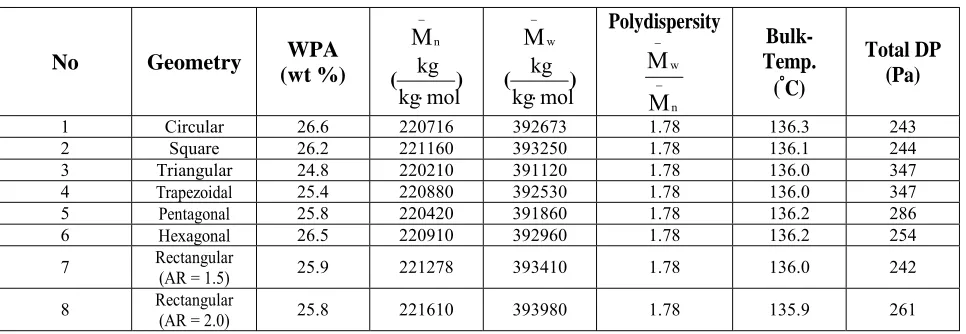
The results obtained in this analysis are indicated in Tables 4 to 8 for the five cases under consideration. In these tables the results of average polymer weight fraction (WPA) in wt % molecular weights (M−n and
−
Mw), polydispersity ( −
Mw/
− Mn) and bulk-temperature (°C) are indicated which are corresponding to the conditions at the exit of the reactors. The total pressure-drop results of the reactors are also indicated. It is observed from these tables that there are only slight differences in the results of conversion obtained for different geometries corresponding to each case. Also the following geometries are observed to provide the maximum conversion for each case:
Case # 1: circular duct (WPA=6.74 wt%; DP = 1.46 Pa).
hexagonal duct (WPA=6.74 wt%; DP = 1.69Pa).
Case # 2: circular duct (WPA=14.2 wt%)
Case # 3: circular duct (WPA=26.6 wt%)
Case # 4: square duct (WPA=57.2 wt%, DP=9078 Pa)
circular duct (WPA=55.2wt %; DP=2617Pa).
Case # 5: 2/1 aspect ratio rectangular (WPA=10.70 wt%; DP=106.6 Pa)
circular duct (WPA=10.10 wt%; DP=50.8Pa).
TABLE 3. Diameter of Circular-Ducts Corresponding to Non-Circular Geometries.
Cases #1 #2 #3 #4 #5
TABLE 4. Simulation Results of Styrene Polymerization at Reactor Exit: Case # 1.
No Geometry WPA
(wt %)
n
M
−) (
mol kg
kg
⋅
w
M
−) (
mol kg
kg
⋅
Polydispersity
n w
M
M
−
−
Bulk-Temp. (°°°°C)
Total DP (Pa)
1 Circular 6.74 452460 819590 1.81 102.3 1.46
2 Square 6.74 452910 820240 1.81 102.2 1.88
3 Triangular 6.38 453450 820660 1.81 101.9 2.70
4 Trapezoidal 6.33 454100 822100 1.81 101.9 2.57
5 Pentagonal 6.63 453810 822110 1.81 102.1 2.28
6 Hexagonal 6.74 452940 820450 1.81 102.3 1.69
7 Rectangular (AR = 1.5) 6.70 453784 821697 1.81 102.0 1.91
8 Rectangular (AR = 2.0) 6.63 455120 823870 1.81 101.8 1.97
TABLE 5. Simulation Results of Styrene Polymerization at Reactor Exit: Case # 2.
No Geometry WPA
(wt %)
n
M
−) (
mol kg
kg
⋅
w
M
−) (
mol kg
kg
⋅
Polydispersity
n w
M
M
−
−
Bulk-Temp. (°°°°C)
Total DP (Pa)
1 Circular 14.2 338740 610770 1.8 106.0 1.05
2 Square 12.7 348550 628480 1.8 104.7 2.52
3 Triangular 11.0 351450 634420 1.8 103.7 6.11
4 Trapezoidal 11.3 352080 635670 1.8 103.7 6.36
5 Pentagonal 12.8 347180 625660 1.8 105.0 2.87
6 Hexagonal 13.6 343910 620230 1.8 105.4 2.76
7 Rectangular
(AR = 1.5) 12.2 351620 634550 1.8 104.1 2.80
8 Rectangular (AR = 2.0) 11.5 356170 643600 1.8 103.3 3.26
TABLE 6. Simulation Results of Styrene Polymerization at Reactor Exit: Case # 3.
No Geometry WPA
(wt %)
n
M
−) (
mol kg
kg
⋅
w
M
−) (
mol kg
kg
⋅
Polydispersity
n w
M
M
−
−
Bulk-Temp. (°°°°C)
Total DP (Pa)
1 Circular 26.6 220716 392673 1.78 136.3 243
2 Square 26.2 221160 393250 1.78 136.1 244
3 Triangular 24.8 220210 391120 1.78 136.0 347
4 Trapezoidal 25.4 220880 392530 1.78 136.0 347
5 Pentagonal 25.8 220420 391860 1.78 136.2 286
6 Hexagonal 26.5 220910 392960 1.78 136.2 254
7 Rectangular (AR = 1.5) 25.9 221278 393410 1.78 136.0 242
8 Rectangular
TABLE 7. Simulation Results of Styrene Polymerization at Reactor Exit: Case # 4.
No Geometry WPA
(wt %)
n
M
−) (
mol kg
kg
⋅
w
M
−) (
mol kg
kg
⋅
Polydispersity
n w
M
M
−
− Bulk-temp
(°°°°C)
Total DP (Pa)
1 Circular 55.2 481130 966680 2.00 101.4 2617
2 Square 57.2 499470 998160 2.00 101.2 9078
3 Triangular 47.4 486550 940300 1.93 101.1 11540
4 Trapezoidal 50.0 489210 953850 1.95 101.2 3625
5 Pentagonal 54.8 492120 979150 1.99 101.2 41568
6 Hexagonal 55.7 487320 976770 2.00 101.4 7574
7 Rectangular (AR = 1.5) 54.1 495730 979780 1.98 101.2 4937
8 Rectangular (AR = 2.0) 48.9 488230 947800 1.94 101.1 1910
TABLE 8 . Simulation Results of Styrene Polymerization at Reactor Exit: Case # 5.
No Geometry WPA
(wt %)
n
M
−) (
mol kg
kg
⋅
w
M
−) (
mol kg
kg
⋅
Polydispersity
n w
M
M
−
− Bulk-temp
(°°°°C)
Total DP (Pa)
1 Circular 10.10 129960 225290 1.73 161.0 50.8
2 Square 9.97 130040 225440 1.73 160.9 67.2
3 Triangular 10.56 130330 225810 1.73 160.8 106.1
4 Trapezoidal 10.30 130380 226000 1.73 160.8 117.0
5 Pentagonal 10.20 130132 225600 1.73 160.9 67.8
6 Hexagonal 10.40 130100 225570 1.73 161.0 64.1
7 Rectangular
(AR = 1.5) 10.20 130250 225810 1.73 160.8 73.9
8 Rectangular (AR = 2.0) 10.70 130430 226000 1.73 160.7 106.6
Therefore, not a specific geometry is recognized to be generally superior to circular duct reactor for the highest conversion of the chemical reaction under study, considering the least pressure-drop results also. The higher pressure-drop of noncircular duct reactors is due to the effect of corners at which the viscosity is tremendously high as observed from the viscosity profile results.
Referring to Tables 4-8, the following relative classification is possible from the conversion point of view based on the circular duct (wt %) results: Case # 1: 6.74 wt %. low conversion
Case # 2: 14.20 wt %. low conversion
Case # 3: 26.60 wt % intermediate conversion. Case # 4: 55.20 wt % high conversion.
Case # 5: 10.10 wt % low conversion.
The reason for the low DP results of cases # 1
and # 2 is due to the low level of conversion involved. The relatively higher values of DP of case #5, which is even at low conversion level, is due to the smaller tube I.D. (0.0046 m) practiced in this case. Typical simulation results for molecular-weights distribution, velocity, temperature, concentration, density and viscosity profiles are presented in Figures 4 to 15 in this section.
An analysis of these figures reveals the following major points:
Figure 4. Case#1 mol. wt distribution (triangle).
Figure 5. Case#1 mol. wt distribution (trapezoid).
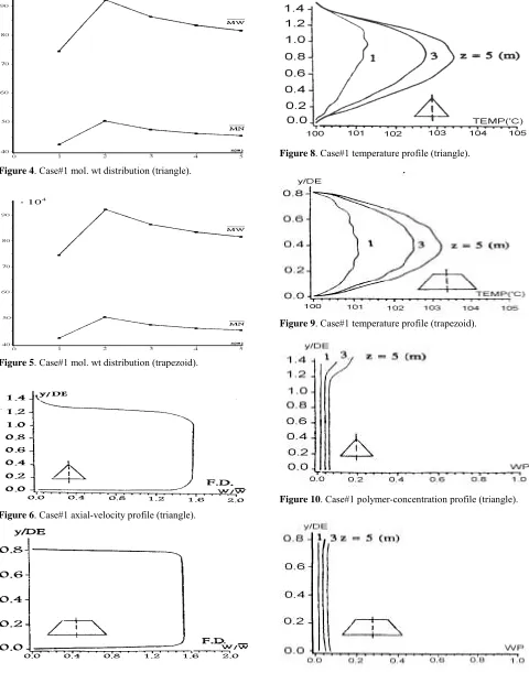
Figure 6. Case#1 axial-velocity profile (triangle).
Figure 7. Case#1 axial-velocity profile (trapezoid).
Figure 8. Case#1 temperature profile (triangle).
Figure 9. Case#1 temperature profile (trapezoid).
Figure 10. Case#1 polymer-concentration profile (triangle).
Figure 12. Case#1 density-profile (triangle).
Figure 13. Case#1 density-profile (trapezoid).
Figure 14. Case#1 viscosity-profile (triangle).
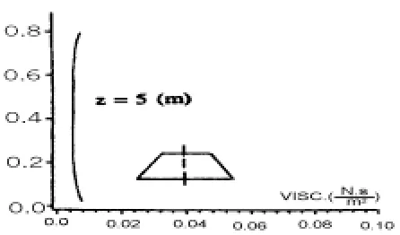
Figure 15. Case#1 viscosity -profile (trapezoid).
the fact that temperature is more uniform transversally at locations closer to the inlet of the reactor due to which the finest quality of polymer is obtained. At downstream locations, however, due to the accumulation of exothermic heat of reaction around the center of the ducts, a non-uniform temperature distribution is generated in transversal-direction, which deteriorates the quality of the polymer product. This is observed by a thereafter-streamwise reduction in the molecular weight results. Typical mol. wt. distributions are shown in Figures 4 and 5 for triangular and trapezoidal duct reactors.
(ii) Axial Velocity Profile
All cases exhibitplug flow behavior which is in close agreement with the prediction of Husain and Hamielec [3]. Some velocity distortion is observed due to the effect of angles as revealed in triangular and pentagonal ducts. This effect is to induce higher rates of generation of polymers at corners rather than at sides due to which the viscosity increases around locations closer to angles. The effect on velocity is a retardation of
velocity profile in the vicinity of the angles. Typical axial-velocity profiles are shown in Figures 7 and 8 for triangular and trapezoidal duct reactors.
(iii) Temperature Profiles
Case # 1: Isothermal reactor exothermic reaction proceeds and the temperature profile is developing to higher values.
Case # 2: Cooled-wall reactor, heat removal is observed from the temperature profile, which is developing to lower values.
Case # 3: Mildly cooled-wall reactor, temperature profile is mildly developing to lower values. Case # 4: Cooled-wall reactor, temperature profile is developing to lower values.
Case # 5: Isothermal reactor, temperature profile is developing to higher values.
Typical temperature profiles are shown in Figures 8 and 9 for triangular and trapezoidal duct reactors.
triangular and pentagonal ducts, an increase in concentration is observed at these locations. Typical concentration profiles are shown in Figures 10 and 11 for triangular and trapezoidal duct reactors.
(v) Density and viscosity profiles
The effect ofangles, is plainly observed in viscosity profiles such that there is a drastic increase in viscosity close to the angles. This is observed in viscosity profiles for the triangular and pentagonal ducts of all cases. The density profiles are also affected to some extent close to these points. The angle effect is the reason for the higher pressure-drop of noncircular duct reactors relative to the circular ones. Typical density and viscosity profiles are shown in Figures 12 to 15 for triangular and trapezoidal duct reactors.
Effect of Free-Convection
Due to the narrow temperature range involved in the transverse direction, the effect of free- convection (buoyancy effect) in this study is found to he negligible. This is observed from the following results, which were obtained, considering free-convection effect for circular ducts corresponding to the results in Tables 4-8.Case # 1: 6.75 wt % conversion. Case # 2: 14.50 wt % conversion. Case # 3: 26.70 wt % conversion. Case # 4: 55.24 wt % conversion. Case # 5: 10.30 wt % conversion.
SUMMARY AND CONCLUSIONS
This paper shows the suitability of a non-orthogonal boundary-fitted coordinate transformation method in the solution of 3D parabolized mass, momentum, energy and species continuity equations in laminar flow and in reacting media in arbitrary cross-sectional duct reactors. The favorable agreement obtained between this numerical solution procedure with the results of other investigators for circular ducts and the absence of convergence difficulties prove the elegant feature of the above-mentioned method. As a novel idea in reaction engineering, the above solution technique is employed to analyze the simulation of styrene polymerization in arbitrary cross-sectional duct reactors. It is observed that not a specific geometry is in general superior than the conventional circular duct reactors considering also the least pressure-drop in the reactors.
NOMENCLATURE
a coefficient in the discretization equation b constant term in the discretization
equations Cp. specific heat
D.L. dimensionless D A mass diffusivity of “A”
Dh,DE hydraulic diameter (or equivalent diameter)
F.D. fully developed
g acceleration due to gravity
I index of “ζ” axis in the transformed plane J index of ‘‘η’’ axis in the transformed
plane
J Jacobian of transformation
k thermal conductivity
k i. rate constant for thermal initiation k p rate constant for propagation
k t r,m rate constant for chain transfer to monomer
kt rate constant for termination
[M] monomer concentration
M apparent viscosity for power-law fluid m, mA monomer (A) weight—fraction
n M N
M , cup average number averaged molecular
weight w
M W
M , cup average weight averaged molecular
weight
n Power-law index
n unit normal vector
P total pressure (dynamic + hydrostatic)
P dynamic pressure
−
P mean viscous pressure
q heat flux
QR heat of reaction
R residual of discretization equation RA mass rate of consumption of reactant “A’’
due to chemical reaction Rp rate of polymerization T temperature
w
v
u
.,
,
velocity components in the Cartesiansystem
U,V,W contra variant velocity components
v velocity field
WPA average polymer weight fraction
−
W
mean axial velocityx, y, z Cartesian coordinate system X m monomer conversion
z reactor length
Greek Letters
∆H heat of reaction
α,β,γ coordinate transformation coefficients
σ
η
ε
,
,
axes of curvilinear coordinateµ
consistency index (for power-law fluids)ρ
densitya
ρ
arithmetic mean density for duct cross— sectionij
∆
rate of deformation tensor ijτ
stress-tensorv
Φ
viscous dissipation function oη
viscosityφ
a general dependent variableSubscripts
nb General neighbor grid point
REFERENCES
1. Sala, R., Valz-Gris, F. and Zanderighi, L., “A Fluid-Dynamic
Study of a Continuous Polymerization Reactor”, Chemical
Engineering Science, 29, (1974), 2205-2212.
2. Wyman, C. E. and Carter, L. F., “A Numerical Model for
Tubular Polymerization Reactors”, AIChE Symposium
Series, Vol. 72, No. 160, (1976), 1-16.
3. Husain, A. and Hamielee, A. E., “Bulk Thermal Polymerization of Styrene in a Tubular Reactor—a Computer
Study”, AIChE Symposium Series, Vol. 72, No. 160, (1976),
112-127.
4. Hui, A. and Hamielee, A. E., “Thermal Polymerization of Styrene at High Conversions and Temperatures, An Experimental Study”,
J. Appl. Polymer Science, 16, (1972), 749-762.
5. Valsamis, L. and Biesenberger, J. A., “Continuous Bulk
Polymerization. in Tubes”, AIChE Symposium Series,
Vol. 72, No. 160, (1976), 18-27.
6. Valsamis, L., and Biesenberger, J. A., “Continuous Bulk
Polymerization of Styrene in a Tubular Reactor”, AIChE
Annual Meeting, N. Y., N. Y., (1977).
7. Chen, C. C., “Polymerization in a Laminar Flow Tubular Reactor”, Ph. D. Thesis, Rensselaer Polytechnic Institute, Troy, N. J., (1986).
8. Chen, C. C. and Nauman, E. B., “Verification of a Complex, Variable Viscosity Model for a Tubular Polymerization
Reactor”, Chemical Engineering Science, 44, No. 1,(1989),
179-188.
9. Kleinstreuer, C. and Agarwal, S., “Coupled Heat and Mass
Transfer in Laminar Flow, Tubular Polymerizers”, Int. J.
Heat Mass Transfer, 29, No. 7, (1986), 979-986.
10. Agarwal, S. S. and Kleinstrener, C., “Analysis of Styrene Polymerization in a Continuous Flow Tubular Reactor”,
Chemical Engineering Science, 41, No. 12, (1986),
2101-3110.
11. Isazadeh, M. A., “Numerical Solution of Reacting Laminar Flow Heat and Mass Transfer in Ducts of Arbitrary Cross-Sections for Power-Law Fluids”, Ph.D. Thesis, McGill University, Montreal. Canada, (1993).
12. Bird, R. B., Stewart, W. E. and Lightfoot, E. N., “Transport Phenomena”, Wiley, New York, (1960).
13. Skelland, A. H. P., “Non-Newtonian Flow and Heat- Transfer”, John Wiley and Sons, NY., (1967).
14. Chu, W. H., “Development of a General Finite Difference
Approximation for a General Domain”, J. Comp. Physics, 8,
(1971), 392 -408.
15. Thompson, J. F., Thames, F. C. and Mastin, C. W., “Boundary-Fitted Curvilinear Coordinate Systems for Solution of Partial Differential Equations on Fields Containing Any Number of Arbitrary Two-Dimensional
Bodies”, Report CR-2729, NASA Langley Research Center,
(1977).
16. Maliska, C. R. and Raithby, C. D., “A Method for Computing Three Dimensional Flow Using Non-Orthogonal Boundary—
Fitted Coordinates”, Int. J. for Numerical Methods in
Fluids, 4, (1984), 519-537.
17. Patankar, S. V. and Spalding, D. B., “A Calculation Procedure for Heat, Mass and Momentum Transfer in
Three-Dimensional Parabolic Flows”, Int. J. Heat Mass Transfer,
15, (1972), 1787-1806.
18. Patankar, S. V., “Numerical Heat Transfer and Fluid Flow”, Hemisphere Publishing Corporation, NY., (1980).
19. Raithby, G. D. and Schneider, G. E., “Numerical Solution of Problems in Incompressible Fluid Flow: Treatment of the
Velocity-Pressure Coupling”, Numerical Heat Transfer, 2,