AIR-FUEL RATIO CONTROL OF A LEAN BURN
SI ENGINE USING FUZZY SELF TUNING METHOD
M . Akhlaghi , F. Bakhtiari Nejad and S. Azadi Department of Mechanical Engineering
Amirkabir University of Technology Tehran, IRAN
(Received: July 20, 1998 - Accepted in Revised Form: April 8, 1999)
Reducing the exhaust emissions of an spark ignition engine by means of engine Abstract
modifications requires consideration of the effects of these modifications on the variations of crankshaft torque and the engine roughness respectively. Only if the roughness does not exceed a certain level the vehicle do not begin to surge. This paper presents a method for controlling the air-fuel ratio for a lean burn engine. Fuzzy rules and reasoning are utilized on-line to determine the control parameters. The main advantages of this method are simple structure and robust performance in a wide range of operating conditions. A non-linear model of an SI engine with the engine torque irregularity simulation is used in this study.
Fuzzy Control, Self Tuning, Engine Roughness, Air Fuel Ratio Key Words
nj k®«pB¼¯ n±U±« º°n oM »UBd¼d~U w±U ºA³ o] » AoTeA n±U±« ð½ »]°oi ºBµ²k®½¿C yµB @
²k¼ña
o¼ ½A ³ »«B¢®µ /k{BM»« n±U±« xjo£ »TiA±®ñ½ o¼ ° ¡®¦¼« n°BTz£ nj RBd¼d~U ½A oYA T o£ o ¯ ³M A±µ SLv¯ ¤oT® ºAoM An »{°n ³§B « ½A /k® »« S oe ¨AnC °nj±i ,k½Bª®¯ p°B\U »®¼í« nAk « pA »TiA±®ñ½ ºBµoTÇ«AnBÇQ ¼¼íÇU ºAoM ¬B«qªµ Rn±~M ºpB ¨±´ « ° ¼¯A± /k® »« ³ÄAnA p±w ¼ n n±U±« ð½ ºAoM Si±w pA »í¼w° ²j°kd« nj ¬C ¨°B « joñ¦ªî° ²jBw nBTiBw x°n ½A pA ²jB TwA »¦æA S½q« /k¯±{»« ³T o£ nBñM ¤oT® @ nB ½A nj n±U±« n°BTz£ »TiA±®ñ½ o¼ ºpBw ³¼L{ BM ºA³ o] n±U±« ð½ pA » i o¼ ¤k« ð½ /SwA ¬C jo nB @ /SwA ²k{ ²jB TwAINTRODUCTION
The most important objective of a fuel control syst em is to provide accurate cont rol of air to fuel (A/F) ratio so that desired drivability and e mission le ve ls can be a chie ve d. F or mo st automobiles, this translates to very tight control near the stoichiometric ratio to maximize the three-way catalyst efficiency. Furthermore , if e ithe r be st economy or maximum power is a priority require me nt for an engine , then t he air-fuel ratio must be respectively quite lean and just rich of stoichiometry. If in the interests of maximum power the air-fuel ratio is quite low and t here is an e xce ss of fuel, t he quality of combustion will be poor and the emissions of bo t h u n bu r n t h ydr o ca r bo n e s a n d ca r bo n
and 21:1 but the gains mentioned are bought at t h e e xp e n se o f in cr e a se d e m issio n s o f hydr ocarbon s an d t he po ssibility o f r ou gh running.
In sum, it will be evident that, the exhaust emissions from an engine are mainly influenced by t he re gion of air-fue l rat io in which it is operating.
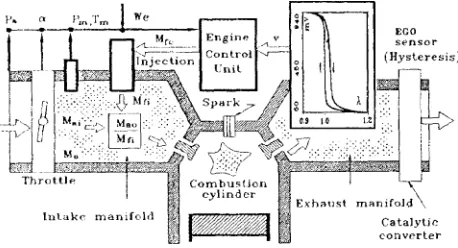
Precise control of the internal combustion e ngine air-fue l ratio is important during all phases of engine operation. During normal hot engine operation the exhaust gas oxygen sensor is u se d wit h in a close d-loo p air-fu e l r at io feedback system to maintain the air-fuel ratio ve ry close t o t he st oichio me t ric va lue . An average air-fuel ratio accuracy of about 0.02 air-fuel ratio units is required[2]. This accuracy is re quired to e nsure t hat t he cat alyst of the a ft e r t r e a t me n t syst e m o p e r a t e s a t h igh conversion efficiency for all three pollutants, i.e. H C, CO , and NO x. This occurs only within a ve r y n a r r o w a ir -fu e l r a t io win d o w. T h e sche mat ic r e pr e se nt a t io n of a clo se d-lo op fuel-injection system is given in Figure 1[3].
There are several methods for controlling the air-fuel ratio. Asik and Meyer [2] estimate t h e a ir -fu e l r a t io ba se d o n in du cin g a n d detecting crankshaft speed fluctuations caused by modulating the engine's fuel injection pulse widths in a predetermined manner. For closed
Fi gure 1 . Schematic representation of closed-loop fuel injection system.
loop control, a conventional PID controller was impleme nt e d. The e rror is calculat e d as the difference be tween the de sired A/F ratio and the estimated A/F ratio.
Nam, Kim and Yoo [3] have pr opose d a fuzzy sliding mode control method for designing a fue l in je ct ion con t ro lle r t o mainta in t he stoichiomet ry air to fuel ratio.This me thod is used because of it's capabilit y to consider the incomplete information of the current oxygen sensor and its applicability to non-linear engine models. The simulation results of this algorithm show good pe rformance re gardle ss of se nsor hysteresis and model errors.
C ho a n d Ke u n O h [4] h ave de signe d a fuel-injection controller based on the theory of va riable st r uct ure syst e ms. This me t h od is formulated t o be compat ible wit h production sensors and actuators, including the switching type feedback sensor.
Inagaki, O hata and Inove [6] developed an adap t ive fue l in je ct io n co nt ro l syst e m for accurate A/F ratio control. This system consists o f a n e st im a t o r o f fu e l b e h a vio r m o d e l pa rame te rs an d a modifie d inte r nal mode l control system with an inverse system.
Also Cho and H edrick [7] have designed a nonline ar sliding mode inje ction controlle r based on a physically motivated, mathematical e ngine mode l. The de signe d controlle r can achieve a commanded A/F ratio with excellent transient properties, which offers the potential for improving fuel economy, torque transients. and emission levels.
SI engine with the large non-linearities of the intake manifold stat e e quat ion is use d in this simulation.
LEAN BURN ENGINE
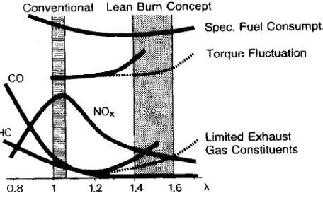
F igu r e 2 Sh o ws in a qu a lit a t ive wa y t h e interconnection between legislat ively limited exhaust constituents. specific fuel consumption, torque fluctuation. and excess air-fuel ratio of the air-fuel mixt ure . At l= 1.4 to l= 1.6 t he N O x e missio n va lu e s ar e a s lo w a s t h o se achie ve d wit h a t hre e way ca t alyst . As t he diagram shows, the specific fuel consumption at le an mixt u re is lowe r t h an l = 1. T his fu e l co n su m p t io n im p r o ve m e n t is t h e m o st significant advantage of the lean burn concept ve r su s a n y o t h e r co n ce p t b a se d o n t h e three-way catalyst.
O t her problems conne ct e d with the le an burn concept are shown in the graph. O ne of t he m is t he sign ifica nt in cr e ase in t or qu e unste adiness which result s in rough running. Another is connected with HC emission, which is higher for lean burn engines than tolerated by most legislative limits, even when the mixture is leaned out. In addition, H C emission increases r ap idly a s t he limit fo r smo ot h r un ning is approached. As can be seen, a lean burn engine needs, aside from measures for exte nding the range for smooth running, measures to reduce HC emissions [5].
A le an burn conce pt doe s not necessarily me an t hat the e ngine must be o pe ra te d at setting ofl>1 across the entire operating range. Mixture metering is achieved as follows:
ÉIdle: preferably l>1
ÉPart throttle: lean control to l>>1
É Full throttle: l <1 or l = 1 to achieve
optimum engine output.
Tuning of production engines shows that idle and part t hrott le se tt ing may be adjuste d t o
Figure 2. Basic trends of exhaust emissions, specific fuel consumption and torque fluctuation as a function of excess air coefficient(l).
givea lean mixture for optimum fuel economy. During acceleration the engine is supplied with a st oichiome tric or rich A/F mixt ure . Whe n designing a lean burn engine two basic criteria have to be taken into account:
1. Operate engine in a specified l range in the lean burn range to keep NOx emissions low. 2. Avoid e xce e ding a ce rt ain leve l of rough run ning or cyclic var iat io n so as t o e nsure correct drivability and to avoid the increase of HC emissions.
If the above criteria are taken into account, a l r a n ge r e su lt s m u st b e a d h e r e d t o b y implementing suitable controls. Figure 3 shows a schematic diagram of thislrange and resulting NOx reduction.
As pointed out above, differe nt st rat egies must be use d for diffe re nt map ra n ge s t o
Figure 4.Block diagram of a lrange formation.
achieve optimum tuning of an engine. Figure 4 shows one way of generating a suitable lrange [4].
ENGINE ROUGHNESS
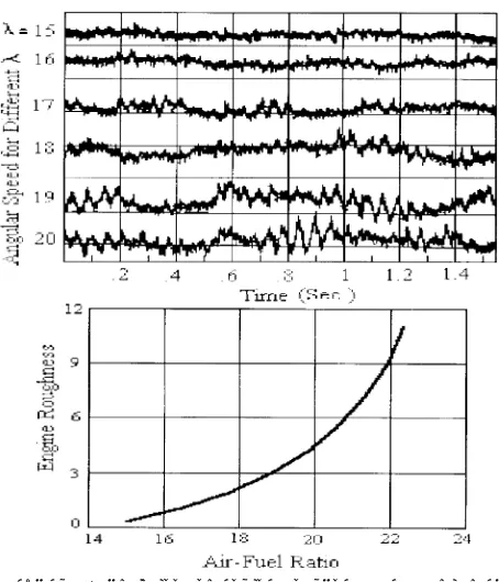
E n gin e r o u gh n e ss is a m e a su r e o f t h e irr e gular it y of t he a n gu la r ve lo cit y o f t h e crankshaft which is cause d by the variation in e ne rgy re lease from cycle t o cycle as we ll as cylinder t o cylinde r. The variat ion of me an effe ctive pressure causes torque changes and results in angular speed changes of crankshaft. The engine roughness corresponds to changes of the me an angu lar acce le rat ion be twe e n s u c c e ss i ve cr a n k s h a f t r o t a t i o n s . I t i s approximately proportional to the change the mean torque or mean effective pressure during one rotat ion of t he crankshaft [8]. F igure 5, sh ows cra nkshaft spe e d for in cre asing t he a ir -fu e l ra t io , wh ich in cr e ase s t he e ngin e roughness. We can also see the optimal ignition point for smooth running in Figure 6, [8-11].
ENGINE MODELLING
Engine modelling efforts for control have been unde rway for le ss than 30 ye ars [12]. The re ha ve be e n man y diffe re nt for mu la t io ns of engine models. In recent years, dynamic models for aut omotive e ngine s have be en de veloped t h a t a r e a ccu r a t e e n o u gh t o be u se d fo r non-linear controllers, but simple enough to be
Figure 5 . Variation of engine roughness versus air-fuel ratio.
Figure 6.Engine roughness as a function of ignition point.
compute d in real time. Some of these models are based e nt ire ly on me asure me nt s and are often refered to as "input-output" models.
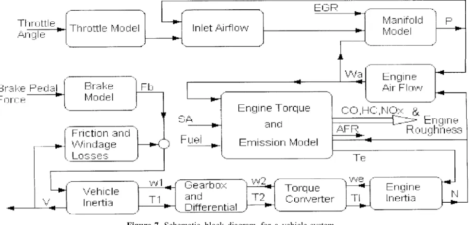
The engine model which is presented here is for var io us p ar t s o f an a ut omobile so a ny dynamic loads and other transients that affect e xhaust e missions and fue l e conomy can be predicted. The vehicle system is divided into the following dynamic subsystem [13,14,15] :
ÉIntake manifold
Figure 7.Schematic block diagram for a vehicle system.
F igure 7, re pre se nts the e ntire mode l in block diagram form. The engine input variables are the throttle angle, the fuel rate, the ignition timing and exhaust gas recirculation (EGR). In t his mode l t he st ate variables are the crank shaft speed and absolute manifold pressure. The engine output variables are the vehicle velocity, exhaust emissions, engine roughness and air-fuel ratio.
Manifold pressure state equation T h e St a t e equation for manifold pressure is obt ained by applying conse rvation of mass. This can be expressed as [14,15]:
(1)
where,
(2) Wth = Wmax . f1. f2. f3. f4
(3) Wmax =
(4) .528 f1= 1 , .528
(5) f2 =
(6) f3 = ___P
P0
(7) f4 =
In constructing the algebraic expression for volumetric efficiency some suggestive results are available in the literature. The function of the volumetric efficiency is [14-17] :
(8) Kp
where,
0.75 Z<1
(9) .75/Z Z 1
The dimensionless parameter Z is identical wit h "Inle t -Valve M ach In de x" a dapt e d by C.F.Taylor, can be written as [15]:
(10) Z=(b/d c)2
The functions kp are given by;
___ 1.4 -.4P Pm
(11) Kp=0 _____ > 1.4 -.4P
Pm
th e ve hicle , t he e ngine de ve lo ps a t o rque de pe nding on air flow, air-fue l ratio, spark advance and other conditions. This torque is t ra nsmit t e d t o wh e e ls t hr ou gh t he t or qu e conve rte r, ge ar box and diffe re ntial. Whe n brake s are applie d, the t hrottle is at its idle position and the brakes decelerate the vehicle dissipating the e xce ss available energy in t he form of h e at . P hysically t he ve hicle ine rt ia equation is derived using Newton's law and can be expressed as:
(12) dv / dt = (Fin - Fout) / Meq
where,
(13) Meq = M + (Iee + Ie ) / R2w
(14) Iee = Ie (GRt)
(15)
(16) Fout = Fr + Cwv2+ Fb
where, Teis a function of throttle angle, spark ignition timing and other engine parame te rs such as air-fuel ratio. The t orque irre gularity from cycle to cycle is expressed by:
(17)
where , is the engine roughness. In this study we have simulated t he engine roughness as a d i s t u r b a n c e o n e n g i n e t o r q u e . T h e ch a r a ct e r ist ics o f t h is sign a l is in go o d a gr e e m e n t wit h e xp e r ime n t a l r e su lt s o f reference [8].
MODELLING OF EXHAUST EMISSIONS
E n gin e o p e r a t in g va r ia b le s a n d d e sign p a ra me t e rs h a ve sign ifica n t influ e nce o n exhaust emissions. It is often difficult to isolate t he e ffe ct s of a single de sign variable or an ope r ating par ame te r. A ny variable such as air-fuel ratio, spark timing, speed, load, E G R , va lve o ve r la p , in t a k e ma n ifo ld p r e ssu r e , compre ssion rat io an d valve t iming have a
significant influence on the exhaust emissions and fuel economy. Many studies have shown that among the me ntione d variables only t he air-fuel ratio, spark advance and E G R can be controlled. Some research workers have used the steady state data from experiment al study and have reported the control strategies which sought to reduce emissions. Some approximate fun ct io n a l r e la t ion sh ip s be t we e n e xh a ust e missions, ope rat ing condit ions and cont rol va r iable s ca n be e st a blish e d. T h e n t h e se empirical relationships can be directly used for de t e r min ing e xhau st e mission ra t e s at a ny operating conditions. The following equations give t h e fu n ct io na l fo r ms for t h e va r iou s emission rates. The functions f1, f2and f3are determined by using the empirical correlation techniques [18].
(18) = f1 (Wth , AFR, , EGR, Te ,n)
(19) = f2 (Wth , AFR, , EGR, Te ,n)
(20) = f3 (Wth , AFR, , EGR, Te ,n)
Because steady state tests are used to obtain the experimental data, these equations are not valid for cold start and warm up periods.
SELF TUNING STRATEGY
Fuzzy control is an old cont rol paradigm t hat has received much attention recently. While a co ntrolle r is at wo rk, u nce rtaintie s such as dist ur ba n ce , p a r ame t e r p e r t u r ba t io n a n d unknown syste m dynamics always exist in t he system. Conventional tuning techniques for PID controlle r usually produce an unsat isfact ory control performance.
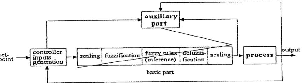
Figure 8.A learning fuzzy controller.
considerable robust effects. A fuzzy controller comp o se d o f co n t r o l r u le s of co n dit io na l lin gu ist ic st a t e me n t s o n t h e r e la t io n sh ip be twe e n input and output variables has t he enticing advantages to emulate the behavior of a human and to de al with model unce rtaint y. Similar t o t radit io n al adap t ive co n t rolle rs, a d a p t ive fu zzy co n t r o lle r s ca n a lso b e categorized into direct and indirect types.
A direct adaptive fuzzy controler can simply be represented by the block diagram as shown in Figure 8, in which the auxiliary part may be a re fe re nce mode l, an auxiliary contro lle r, a mo nit or , or a p ara me t e r a dju st e r, a nd t he diagonal line across the basic part me ans t he tuning process upon the fuzzy controller.
T he r e fe re nce mo de l is co nst ru ct e d by defining a desired dynamic equation or by using the relationship between change in input and change in output error.
In t his st udy t he o bje ctive of t he fuzzy controlle r is t o t rack the vehicle velocit y and co n t r o l t h e A /F r a t io in le a n o p e r a t in g conditions. So the desired A/F ratio is obtained by the exhaust emissions and engine roughness limit ed. In t his paper we have used the fuzzy tuning me thod for a djusting the con trolle r parameters. The controller only requires input and output data ( does not require the plant's m o d e l) . T h is me t h o d is b a se d o n se r vo con t rolle r tuning with fuzzy logic which is
Figure 9.The block diagram of integrated controller.
adapted by H.C Tseng and V.H. Hwang [19]. F igure 9. shows block diagram of t he self tuning fuzzy control. u is the plant input vector, y is t he ou tpu t ve ct or, yd( t ) is t he de sir e d output vector and e is the error vector.
The Process model is written by:
(21) (t) = f (x(t), u(t),t)
(22) y(t) = g( (t), x(t),t)
(23) e(t) = y(t) - yd(t) for tracking
(24) u(t) = Ke(t)
(25) where, xû Rn , uû Rm , yû Rr , eû Rr.
The tracking tuner cases that:
(26) e(t) 0
FUZZY RULES
The control variable u( t ) is proportional t o error e(t) and is given by:
(27) u(t) = K(t) e(t)
The objective of the fuzzy tuner is to evaluate the incremental changes of K. In other words, we have:
Based on the servo controller tuning whose complet e t echnique can be found in [19], we have used the method for fuzzy rules generation b a se d o n t h e L ya p u n o v f u n c t io n a s a pe rformance inde x. Conside r t he following Lyapunov funct ion candidate for de riving a stable fuzzy rule set [19,20]:
(29) V(e, )= eT e +
The rate of change of V with respect to time, , can be approximated by:
(30)
where, DV (tk) = V(tk) - V(t
k+1). In order to
drive yid(t), we require . To satisfy the condition or by tuning K, one must find an expression that relates D
to the desired changes in K. This expression can be obt aine d t hrou gh t he intr oductio n of a sensitivity function:
(31)
which leads to:
(32)
and for a stable control,
(33)
The ide a of de riving t he fuzzy rule s is t o have such that it converges at a constant rate , where is a positive defining the convergence rate. To guarantee this convergence condition, on can use the principle of superposition to determine the sign of each Kij ,such that is always negative.
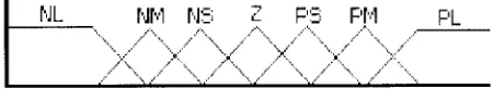
One way to fuzzify the variables, ei , Kij a n d Sij is t o in t r o du ce a lin gu ist ic t e r m (membership function) for each of them in form of triangular as is shown in F igure 10. The complete fuzzy decision table for the matrix K is as shown in Table 1. In this paper the quadratic
Figure 10.Membership function for the fuzzy term sets.
TABLE 1. Fuzzy Decision Table for Matrix K.
PL PM PS Z NS NM NL Sij PM PM PS Z PS PS PS NL PL PM PM PS PS PM PM NM PL PL PM PS PM PM PL NS Z Z Z Z Z Z Z Z NL NL NL NM NM NM NL PS NL NM NM NS NS NM NM PM NM NS NS Z NS NS NS PL
performance index is as follow:
(34) J = eT Qe + P
where, e is output error vector and Q and P are we igh t in g m a t r ix fo r se le ct in g t h e mo st important outputs.
RESULTS AND DISCUSSIONS
Figure 11.Air-fuel ratio versus time.
Figure 12.The engine fuel consumption rate.
Figure 13.Throttle angle position versus time.
engine operated at rich mixture. Therefore, the r e q u ir e m e n t s o f t h e b e st e co n o m y a n d maximum power are satisfied.
CONCOLUSION
In t his p ap e r, it h as be e n sh own t ha t it is possible t o find the be st e ngine adjustme nt compromise re garding emissions and engine
Figure 14.The tracking control of vehicle velocity.
roughness. A vehicle model has been used for simula tion. T he mode l contains non-line ar e le me nt s of t he e ngine , spe cially the e ngine t orque irre gularit ie s. The cont rol is done by regulating the multidimensional proportional fuzzy controller gains. These simulation results showe d t he applicabilit y of se lf tuning fuzzy control for air-fuel ratio control to a lean burn engine.
NOMENCLUTURE
Area of throttle body throat (m2) Atm
Air to fuel ratio AFR
Sound speed (m/sec) a
Piston diameter (m) b
Flow coefficient of throttle body throat Cdt
Air flow coefficient in inlet valve Ci
Drag coefficient Cw
Co exhaust emission rate o
Inlet valve diameter (m) dc
Exhaust gas recirculation EGR
Positive force at the wheel (N) Fin
Negative force at the wheel (N) Fout
Braking force (N) Fb
Friction force (N) Fr
Axle ratio G
Hc exhaust emission rate H
Moment of inertia of rotary parts (kgm2)
Ie
Equivalent moment of inertia (kgm2)
Iee
Inlet valve closing angle (degree) Ivc
Ratio of specific heats k
Vehicle mass (kg) M
Equivalent mass (kg) Meq
nm Average of piston speed (m/sec) N Nox ehaust emission rate
P Exhaust pressure (kpa) Po Standard pressure (kpa) Pm Intake manifold pressure (kpa) R Ideal gas constant (KJ/kg.K) Rt Transmission gear ratio Rw Wheel radius (m)
T Exhaust temperature (K) Te Engine output torque (Nm) To Standard temperature (K)
Tm Intake manifold temperature (K) V Displaced volume of engine (m3)
Vm Intake manifold volume (m3)
v Vehicle speed (m/sec)
Wth Throttle mass air flow (kg/sec)
WmaxM a ximu m ma ss a ir flo w in t o in t a ke manifold (kg/sec)
Z inlet mach index
a Throttle angle (degree) e Compression ratio d Spark advance (degree) dn Engine roughness (1/Sec2) l excess air coefficient
zt Mechanical efficiency of gear box hv Volumetric efficiency
REFERENCES
N e wt on, K., St eeds, W ., G ar r e t t , T . K., "T he m ot or 1.
vehicle", Butterworth-Heinemann, (1991).
Asik, J. R., Meyer, G. M. and Tang, D. X . , "A/F ratio 2.
e st im a t io n a n d con t r o l b a se d o n in d u ce d e ngin e r o u gh n ess"IEEE Control Systems, P P . 35-42, ( D e c. 1996).
Nam, S. K., Kim, J. S. and Yoo, W. S., "Fuzzy sliding 3.
mo de co ntr ol of gaso lin e fu el ignit ion syst em with oxygen sensor ",JSME InternationalJournal, Ser ies C, Vol. 37, No. 1, (1994).
D an Cho , D . H . a nd O h, H . K., "Variable stru ctu re 4.
control method for fu el injected systems",Journalof Dynamic Systems, Measurement and Control, V ol. 115, pp. 475-481, Sep.(1993).
Seiffert, U. and Walzer, P . , "Automobile technology of 5.
the future", SAE Publication, (1991).
Inagaki, H., Ohata, A. and Inove, T., "An adaptive fuel 6.
injection contr ol with internal model in au tomotive engine",IEEE Paper, (1990).
Cho , D . and H ed rick, J .K., "A non linear cont roller 7.
design me thod for fuel inject e d a ut omotive e ngines", Journal of Eng. For Gas Turbine and Power, Vo l. 110, pp. 313-320, (July 1988).
Lat sch, R . a nd M a usner , E ., "E xper ience s wit h a ne w 8.
method for measuring the engine rou ghness",ISATA, Vol. 2, pp. 306-319, (1979).
A k h la g h i, M . , B a m e r , F . a n d L e n z , H . P . , 9.
"E xp e rim en t al st u die s o n lea n r u n spa r k ign it io n engines with intensive micro turbulence", ISATA, Graz, Vol. 2, pp. 113-121, (Sep. 1979).
Bamer, F., Lenz, H. P . and Akhlaghi, M., "The effect 10.
of mean pressure variations on the angular velocity on t h e r u n n in g d ist u r b a n ce a n d o n o t h e r p o ssib le measured quantities", ISATA, Vol. 1, pp. 502-518, (Sep. 1979).
Akhlaghi, M ., "Lau fu n r u he , Abga se m issione n u nd 11.
Verbrau ch eines O ttomotors bei Magerbetrieb u nd M o e glich k e it e n zu r Au swe it u n g d e s m a ge r e n Betriebsbereiches", VWGO, Wien, (1978).
P owe ll, J. D ., "A r e vie w o f I C e ngine mo d e ls fo r 12.
co n t r o l syst e m d e sign ", IFAC 10th Triennial Word Congress, Munich, FRG, (1987).
D o bn er , J. D ., "A ma the ma tica l e ngin e m od el for 13.
development of dynamic engine control",SAEPaper No. 800054, (1980).
Coat s, F . E . and F ru echt e, R . D ., " D ynam ic engine 14.
mod els for cont rol deve lopm ent - pa rt I I",Int. J. of Vehicle Design, (1983).
H en d ricks, E . a nd So r en son , S. C., "M ea n V a lu e 15.
Modelling of Spark Ignition E ngines",SAEPaper No. 900616, (1990).
Nagao, F ., "Nishiwaki K. and Yokoyama F.,"R elation 16.
b et we en inle t va lve clo sin g a n gle an d vo lu m e t ric efficiency of a four stroke engine",Bulletin JSME, Vol. 12, No. 52, (1969).
H ara, S., Nakajima, Y. and Nagu mo, S., "E ffects of 17.
intake - valve closing timing on spark ignition engine combustion", SAEPaper No. 850074, (1985).
H a sse l, P . J. D ., Jou mar d, R . an d H ickm an, A. J ., 18.
"Vehicle emissions and fu el consu mption modelling based on continuous measurements", FisitaPaper No. 945127, (1994).
Chr is T se ng, H . a nd H wang, V. H ., "Se r vo cont roller 19.
tu ning with fu zzy logic",IEEE Transactionson Control Systems Technology, Vol. 1, No. 4, Dec. (1993). W a n g, Li-xin , "St a b le a d a p t ive fu zzy co n t r o l o f 20.