Predictive Controlled GSP Performance Improvement with an Integrated ℋ2/ℋ∞ (TECHNICAL NOTE)

(1)

International Journal of Engineering

J o u r n a l H o m e p a g e : w w w . i j e . i r

Predictive Controlled GSP Performance Improvement with an Integrated

_ℋ

2

/

ℋ

∞

M. Rezaei Darestani*a_{, A. A. Nikkhah} a_{, A. Khaki Sedigh} b

a_{Aerospace Department, Khaje Nasir Toosi University of Technology, Tehran, Iran}

b _{Electrical and Computer Department, Khaje Nasir Toosi University of Technology, Tehran, Iran}

P A P E R I N F O

Paper history:

Received 25 December 2012

Recivede in revised form 21 January 2013 Accepted 28 February 2013

Keywords: 3 Axis GSP Predictive Control ℋ2/ℋ∞ Control

A B S T R A C T

An integrated robust optimal control is presented to enhance the closed loop performance in the presence of disturbance and uncertainties, to ensure smooth tracking and elimination of high frequency disturbances especially in accurate systems with minimum power consumption. Simulation result of the proposed controller based on the combination of ℋ2 and ℋ∞ controllers is used to show the

effectiveness of the proposed methodology. A 3 axis gyro-stabilized MIMO platform is considered and the results of the NLPID and a single ℋ∞ controller are compared with the proposed ℋ∞/ℋ2

controller.

doi:10.5829/idosi.ije.2013.26.11b.04

NOMENCLATURE

D Damping coefficient about output axis Tni Net input torque of related axis

i

F Servo-amplifier transfer function UC Control input

y

H Angular momentum of y axis gyro Uf Desired applied input

z

H Angular momentum of z axis gyro U₀ Reference input

i

I Total moment of inertia about output axis UPi Net applied output torque

i

J Total moment of inertia about input axis YP Plant output

K Spring constant about output axis Greek Symbols

( , )

k x t External structured disturbance nonlinear dynamic s_i Absolute angular motion about output axis

( , )

n x t Unstructured external disturbance nonlinear dynamic

1. INTRODUCTION1

Robust control is a prescribed solution to the control of uncertain systems with various affecting disturbances. In recent years, the ℋ2 and ℋ∞ controller design techniques have been widely studied. Both have strong theoretical basis and are efficient algorithms for synthesizing optimal and robust controllers. Their combination, the mixed ℋ2/ℋ∞ allows combining intuitive quadratic performance specifications of the ℋ2

*_{Corresponding Author Email:} _{[email protected] (M. Rezaei}

Darestani)

synthesis with robust stability requirements specifications expressed by the ℋ∞ synthesis. Integration of these controllers leads to a superior closed loop performance in the presence of large uncertainties and disturbances [1-4].

Many difficulties in the integrated ℋ2/ℋ∞ controller design exist, where the straightforward combination of the ℋ2 with the ℋ∞ methodologies results in a conservative solution, i.e. the algorithm may fail to find a controller even if one exists, or it may be possible to find another controller, which achieves better values for the two norms. In this paper, a mixed

ℋ2/ℋ∞ controller synthesis technique based on linear

(2)

matrix inequalities (LMIs) to setup a dynamic output feedback controller with transformed input is proposed [5-7].

The proposed model in this paper is a 3 axis gyro-stabilized platform (GSP) that because of high sensitivity in stability, tracking and control performance requires a controller that considers all disturbances and uncertainties which exist in input, output or state of the system. Small errors in the control system in compensation of disturbances or uncertainties cause great integral error in long term for the whole system. These errors affect system setting and finally system design accuracy.

In this paper, a predictive controller combined with an integrated ℋ2/ℋ∞ controller is proposed. This combination increases the performance and stability, compensates system disturbances in the presence of unmodeled system uncertainties and disturbances. There is a rich literature in this area of control system design. These studies include, robust output feedback controller for the mixed ℋ2/ℋ∞ controller. Based on Genetic Algorithms (GAs) and linear matrix inequalities (LMIs), a hybrid algorithm for uncertain continuous-time linear systems is presented [1]. To overcome the need for multivariable method of designing controller of low order, direct reduced order mixed ℋ2/ℋ∞ control for the short take-off and landing maneuver technology is demonstrated. [8]. Mixed ℋ2/ℋ∞control problem with reduced order controllers for time-varying systems in terms of the solvability of differential linear matrix inequalities and rank conditions is provided [9]. A mixed ℋ2/ℋ∞ controller synthesis technique based on multi-objective optimization is used, where the optimized criteria are the ℋ2 and ℋ∞ norms. The method is compared with the existing methods for solving linear matrix inequalities (LMIs) and bilinear matrix inequalities (BMIs) [5]. For a class of singular problems, necessary and sufficient conditions are established, so that the posed simultaneous ℋ2/ℋ∞ problem is solvable by state feedback controllers [6]. Fixed-structure discrete-time ℋ2/ℋ∞ controller synthesis problem in the delta operator frame work is considered [7]. A new approach to mixed ℋ2/ℋ∞ output feedback control synthesis is proposed. Use of non-smooth mathematical programming techniques to compute locally optimal ℋ2/ℋ∞ controllers, which may have a pre-defined structure, is presented [2]. A robust hybrid motion/force controller for rigid robot manipulators is presented. The main contribution of this study is that the proposed hybrid control system is able to accomplish motion objectives in free directions and force objectives in constrained directions under parametric uncertainty both in robot dynamics and stiffness constraint constant [10]. LTI and qLPV

ℋ2/ℋ∞ controllers are compared. The Pareto limit is used to show the compromise that has to be done when

a mixed synthesis is achieved [3]. A stochastic ℋ∞ and a mixed, stochastic, ℋ2/ℋ∞ control problem for discrete-time systems are considered and solved. Conditions for existence of a solution are derived, based on the solvability of an equivalent mini-max problem [4]. A collection of methods for improving the speed of MPC, using online optimization is described. These custom methods, which exploit the particular structure of the MPC problem, can compute the control action on the order of 100 times faster than a method that uses a generic optimizer [11], and so on [12-16].

Here a special combination of robust optimal control to have a smooth tracking, a model predictive controller (MPC) and an integrated ℋ2/ℋ∞ control to high frequency disturbance rejection with a transformed input vector of cost function in a 3 axis coupled GSP is proposed.

This paper is organized as follows. In section two, 3 axis GSP model is derived. In section three, robust and optimal control theory and their combination is extended. In section four, the simulation results of the robust optimal methodologies to control and stabilize the system are demonstrated and finally results of the proposed controller with nonlinear PID (NLPID) and single _ℋ∞ control are compared.

2. THREE AXIS GSP MODELING

With the use of mechanical gyros in a GSP structure, its model has been derived. The mathematical model of the mechanical gyro is based on the Euler equation of motion for a solid object where its center of mass is located on its center of rotation. Symbolic equation of motion is [17]:

M=H&+ ´w H ₍₁₎

The equation of motion of a single axis gyro with output axis q_z and the input axis f_y and the input-output axis moments (T_n-U_P) is as follows [17]:

(2)

2

. . . .

n y y z

T =J s f +H sq

(3)

2

. . ( . . )

p y z

U = -H sf + I s +D s K+ q that gives

(4) 2

( . . . . )

z

n y y y z

H

T J J s H s

q

f q

=

+

and hence

(5)

2_. n

y y

T s

J

f =

(6)

2

( .I s +D s K. + )qz=H s. .fy+Up

(3)

; ; y y n z z z

x u T y

f f q q q é ù ê ú ê ú

=_{ê ú} = =

ê ú ê ú ë û & & (7) gives: (8) 0 0 0 1 0 0

0 1 0 0 0 0

0 0 0 0 1

0

0 ₀ p

x x J u

U

H K D

I I I I

é ù é ù é ù ê ú ê ú ê ú ê ú ê ú ê ú ê ú

=ê ú +ê ú +

ê ú ê ú

ê ú

ê ú ê ú

ê _- _- ú

ê ú ê ú

ê ú

ë û ë û ë û

&

(9)

[

0 0 1 0

]

y= x

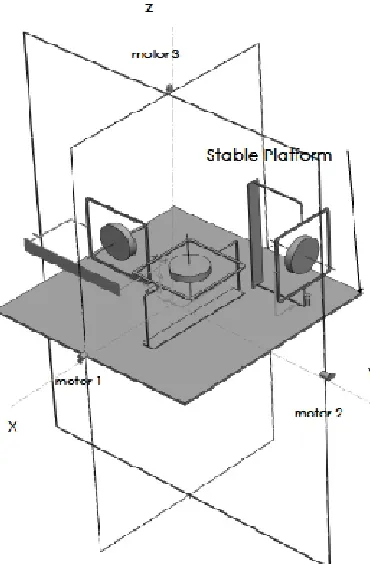
This type of gyro stabilized platform consists of 3 single axis stabilizers. In this arrangement sensitive axis of each gyro is in direction of each axis of the stabilized platform. In relation to the sensed deviation of input axis of gyro, moment has been exerted to the related axis of platform to stabilize that axis. The main problem of a 3 axis GSP is input and output axis coupling of each channel. In this stabilizer which its schematic view and gyros structure is shown in Figures 2 and 3,

q

angle is related to the precision axis and f is related to the rotation of input axis of stabilized platform gyros. As the structure of gyros on the platform is as Figure 3, the output angle of 3 axes is derived as the Equations (16) to (18). By considering axis coupling and use of single axis stabilized gyro, equation of motion of 3 axis gyro stabilized platform has been derived for each channel [17].

X channel:

(10)

2_. nx

x y T s J f = (11) 2

( .I s +D s K. + )q_z=H s_y. .f_x+U_p

Y channel:

(12) 2_. ny

y y T s J f = (13) 2

( .I s +D s K. + )q_x=H s_z. .f_y+U_p

Z channel:

(14)

2_. nz z y T s J f = (15) 2

( .I s +D s K. + )q_y=H s. .f_z+U_p

and considering the channels coupling of the stabilized platform, the channels outputs are:

x z z

s =q +f (16)

y x x

s =q +f (17)

z y y

s =q +f (18)

Also, the control signals and the disturbances of each channel are respectively, (i: x, y, z) [17]:

ni di si

T =T -T (19)

.

si i i

T =F s (20)

As previously stated, the input moment causes precision of gyro to sense the

q

angle. This sensor is installed in each channel of the stabilizer and the state space equation of a three axis platform is derived as follows:

(21) f

X& =AX BU U+ +

(22)

Y CX=

(23) ; ; é ù ê ú ê ú ê ú ê ú ê ú ê ú

ê ú _é _ù _é _ù _é ₊ _ù ê ú _ê _ú _ê _ú _ê _ú ê ú

=_ê _ú =ê ú =ê ú=ê + ú ê ú ê ú ê ₊ ú ê ú ë û ë û ë û ê ú ê ú ê ú ê ú ê ú ê ú ê ú ë û & & & & & & x x x x y

nx x z z

y

ny y x x

y

y y

n z z

y z z z z T

X U T Y

T f f q q f

s q f

f

s q f

q _q _f

s q f f q q (24)

0 1 0 0 0 0 0 0 0 0 0 0

0 0 0 0 0 0 0 0 0 0 0 0

0 0 0 1 0 0 0 0 0 0 0 0

0 0 0 0 0 0 0 0 0

0 0 0 0 0 1 0 0 0 0 0 0

0 0 0 0 0 0 0 0 0 0 0 0

0 0 0 0 0 0 0 1 0 0 0 0

0 0 0 0 0 0 0 0 0

0 0 0 0 0 0 0 0 0 1 0 0

0 0 0 0 0 0 0 0 0 0 0 0

0 0 0 0 0 0 0 0 0 0 0 1

0 0 0 0 0 0 0 0 0

H K D I I I

A

H K D I I I

é ù

ê ú

ê - - ú

ê ú

= ê ú

ê ú - -ê ú ê ú ê ê ê ê ê

ê _-

-êë û

0

1 ₀ ₀

0 0 0

1

0 0

,

0 0 0

1

0 0

0 0 0

x x x J J B J é ù ê ú ê ú ê ú ê ú ê ú ê ú ê ú ê ú ê ú ê ú

= ê ú

ê ú

ú _ê _ú

ë û (25) 0 0 0 0 0 0 0 0 0 px x f py y pz z U I U U I U I é ù ê ú ê ú ê ú ê ú ê ú ê ú ê ú ê ú ê ú ê ú ê ú = ê ú ê ú ê ú ê ú ê ú ê ú ê ú ê ú ê ú ê ú ê ú ë û

0 0 1 0 0 0 0 0 1 0 0 0 1 0 0 0 0 0 1 0 0 0 0 0 0 0 0 0 1 0 0 0 0 0 1 0

C

é ù

ê ú

= ê ú

ê ú

ë û

(4)

A controller to stabilize and ensure closed loop tracking of the MIMO linear time invariant model of the gyro-stabilized system must now be designed. Hence, output control of 3 axis stabilizer has been derived [17]:

(27)

0 c

U=U -U

(28)

.

C

U =F Y

(29)

1

2

3

0 0 0 0 0 0

F

F F

F

é ù

ê ú

= ê ú

ê ú

ë û

Figure 1. Gyro axis orientation on platform

Figure 2. Schematic of 3 axis stabilized platform

Figure 3. Proposed controller block diagram for the stabilized platform

3. GSP CONTROL IDEA

The proposed controller for the 3 axis GSP is an integrated controller that is a combination of ℋ2/ℋ∞ in the inner loop and predictive control in the outer loop, which added integral/derivative of platform attitude to cost function parameters vector.

This combination uses benefits of predictive control to have a smooth tracking and reduction of low frequency time variant disturbances of a pre-defined trajectory, and a mixed ℋ2/ℋ∞ controller to handle unknown uncertainties and compensating high frequency disturbances with minimum control force with the use of LMI theory.

Also, in predictive control with considering instantaneous receding horizon, system could overcome the sudden increase of input control signal and instability. Figure 4 shows block diagram of the proposed controller for the 3 axis GSP [18-20].

4.INTEGRAL/DERIVATIVE PREDICTIVE CONTROL

Predictive control is an optimal controller and provides high accuracy in tracking of the desired trajectory. The stabilized platform could reach to a high accuracy with proper selection of sensors and the selected structure of optimal controller. In the second step, with implementation of input commands, in the case of output disturbances, could reach to the desired accuracy of the system. In what follows, the cost function of the model predictive control (MPC), and the integral/derivative characteristics of the error are given. To design the predictive control state, space equation of the 3 axis GSP is used [14-16]:

(30)

( , ) . ( ) . ( )

X& =F X U =A X t +BU t

(31)

( ) .

x

y

z

Y G X C X

s s s

é ù

ê ú

=_ê _ú= =

ê ú

ë û

Uc UMPC

Yp

IDMPC PLANT

ℋ2/ℋ∞

Controller

(5)

To control the stabilized platform, it is assumed that the proposed platform is fixed on a set point or moves with an external command U_Pi (usually U_Pi »0 in controller design) to a defined position. So a predefined trajectory for equation of motion of body without disturbances in ideal condition as the reference model is considered [14- 16]:

(32)

( ) ( , ) . ( ) . ( )

r r r r r

X t& =F X U =A X t +BU t

(33)

( ) .

r r r

Y =G X =C X

where U_ri is the input reference moment and Y_ri is the output reference angle in each axis of the stable platform. This reference model has been used to define control input variations of the system in all conditions with or without disturbance. With these two defined models the error equation of the system is derived [12]:

(34)

( ) ( , ) . ( ) . ( )

X t&_V =F X U_V _V =AX t_V +BU t_V

(35)

( ) .

Y_V =G X_V =C X_V

Now to reach to the desired control specifications, output error vector which consists of integral and derivative of the output error is:

(36)

( )

x x xr

y y yr

n

y y yr

z z zr

dt dt

Y H X

dt dt

V

t s s

-é ù é ù

ê ú ê _- ú

ê ú ê ú

ê ú ê _- ú

ê ú ê ú

ê ú ê _- ú

ê ú ê ú

-ê ú ê ú

= = =

ê ú ê ú

-ê ú ê ú

ê ú ê _- ú

ê ú ê ú

ê ú ê _- ú

ê ú ê ú

ê ú ê - ú

ë û ë û

ò

%

&% & & %

%

&% & &

% %

%

&% & & %

In the steady state, as

₍

t® ¥

₎

, the output controlled error tend to reach to zero

₍

YV®0

₎

and decreases the

error of the whole system, as the system output tracks the reference path. The proposed controller is optimal with minimum energy consumption and could compensate output error changing. This condition with minimizing the following cost function in the proposed MPC has been assessed [14-16]:

(37)

{

}

[ ] [ ] [ ]

. [ ] ( | ) ( | )

r r r

r r

Jz Y Y Q Y Y u u

R u u Y k N k Y k N k

V V V V V V

V V V V

= - - +

-- + W + - +

% % % % _% _%

% %

where R and Q are diagonal positive definite weighting matrices, and N is the control horizon. Also W is the cost of final states in the predictive system which is explained as [12, 16]:

(38)

{

( | ) ( | )

}

[ ( | )

( | )] .[ ( | ) ( | )]

r

r r

Y k N k Y k N k Y k N k Y k N k Q Y k N k Y k N k

V V V

V V V V

W + - + = +

-+ + - +

% % %

and in the above equation QV is positive definite. Output

prediction of the future step of discrete model of the system is [14, 15]:

(39)

( 1| ) ( | )

ˆ

( 1| ) ( | )

r r

u k k u k k

u

u k N k u k k

V V

V

V V

é + - ù

ê ú

= ê ú

ê _{+ +} _- ú

ë û

% %

% M

% %

(40)

( 1| ) ( | )

r r

Y k k Y k k Y

Y k N k Y k k

V V

V

V V

é + - ù

ê ú

= ê ú

ê _{+ +} _- ú

ë û

% %

% _M

% %

and

(41)

1

2 2

k

N k N

CA Y

Y CA

X

Y _CA

V

+

é ù

ê ú

ê _{ú =} ₊

ê ú

ë û ë û

% M M

1

ˆ

0 0

ˆ 0

.

ˆ 0

k

N N L

k L

u CB

CAB CB u

CA B CA B _u

V

+

-

-+

é ù

é _{ù ê} _ú

ê _{ú ê} _ú

ê ú

+_ê _ê _ú

ú ê ú

ê _{ú ê} _ú

ê ú

ë _{û ë} _û

% L

L %

M M L M M

L %

Minimizing the cost function of the predictive control without the constraints results in the following control law and this control signal has been used in the input control signal of the equation of motion of the system [12, 14-16]:

(42)

[ ]1

(

)

ˆ _' _. _' ˆ_r _{( )} ˆ_r

u%V = H QH R+ - _ë_êéH Q YV -S X kV V +Ru%V ù_ú_û

which in every sampling time, k, only _uˆ_%_V_{signal is} required and finally the resulted control signal has been used in the GSP to reach an appropriate tracking.

5. MIXED ℋ2/ℋ∞ CONTROLLER

In this section, an integration of a special type of robust optimal control, a mixed _ℋ2/ℋ∞ control is presented. This control system stabilizes the stable platform and must compensate all the unknown high frequency disturbances in the tracking loop of the predictive control with minimized control effort. This process must consider the optimal control signal boundary of the system especially in the presence of disturbances. We have [12, 21]:

(43)

2 2 u

X&=AX B w+ _{¥ ¥}+B w +B U

(44)

2 2 u

Z¥ =C X D w¥ + ¥¥ ¥+D w¥ +D U¥

(45) 2

2 2 2 22 2 u

(6)

(46)

2 2

y y y yu

Y C X D w= + ¥ ¥+D w +D U

where

U

is the input control vector, w₂ is the external structured disturbance vector, w_¥is the unstructured external disturbance vector, and X, Y and Z are the state and output of the system. Let Dyu=0 and to compute a finite value of the ℋ2 norm D22 =0 and also generally

2 2 0

D¥ =D¥= , so [20-22]:

(47)

2 2 u

X&=AX B w+ _{¥ ¥}+B w +B U

(48)

u

Z¥=C X D w¥ + ¥¥ ¥+D U¥

(49) 2

2 2 u

Z =C X D U+

(50)

2 2

y y y

Y C X D w= + ¥ ¥+D w

For high frequency disturbance attenuation, control of the first order derivative of platform attitude has been considered. Also, as in MPC, proportional, derivative and integral sequence of rate of change of platform attitude error has been considered in the error vector. The integral term accomplishes zero steady state error when steady disturbance error affects the system. For the case of output-feedback, a dynamic controller is assumed for each part of the ℋ2 and ℋ∞ controller. For the _ℋ2 controller:

2 Ak2 2 B T yk2 1 c1

z& = x + _% ₍₅₁₎

2 k2 2 k2 1 1

U =C z +D T y%_c (52) and for the ℋ∞ controller:

2 2

k k

A B T y_c

z&¥= ¥ ¥x + ¥ % (53)

1 2

k k

U¥=C¥ ¥z +D T y¥ %c (54)

: ki ki

Ci ki ki A B K C D é ù ê ú

ë û (55)

In the first step to design this controller, to stabilize the system in the inner loop and compensation of high frequency disturbances, the output error considered for the above outputs are:

(56)

1 11 1

( )

.

x _x _xr

x x xr

y y yr

y yr y y yr y z zr z z zr z z zr z dt dt

y C x

dt dt

c c

c _s _s

c s s

s s c s s c s s c s s c s s c

é ù _é _- _ù

ê _{ú ê} _ú

-ê _{ú ê} _ú

ê _{ú ê} _ú

-ê _{ú ê} _ú

ê _{ú ê} _ú

-ê _{ú ê} _ú

ê _{ú ê} _- _ú

ê ú

= =_ê _ú=

ê _{ú ê} _ú

-ê _{ú ê} _ú

ê _{ú ê} _ú

-ê _{ú ê} _ú

ê _{ú ê} _- _ú

ê _{ú ê} _ú

ê _{ú ê} _- _ú

ê ú ë û

ë û

ò

%

&% & &

%

& & & % % % % % & & &% % (57) 11

0 0 0 1 0 0 0 0 0 0 0 0 1 0 0 0 0 0 0 0 0 0 1 0 0 0 0 0 0 0 0 1 0 0 0 0 0 0 0 0 0 1 0 0 0 0 0 0 0 0 1 0 0 0 1 0 0 0 0 0 0 0 0 1 0 0 0 0 0 0 0 0 0 1 0 0 0 0 0 0 0 0 1 0 0 0 0 0 0 0 0 0 1 0 0 0 0 0 0 0 0 1 0 0 0 0 0 0 0 0 0 0 0 0 1 0 0 0 0 0 0 0 0 1 0 0 0 0 0 0 0 0 0 1 0 0 0 0 0 0 0 0 1 0 0 0 0 0 0 0 0 0 1 0 0 0 0 0 0 0 0 1

C é ù ê ú ê ú ê ú ê ú ê ú ê ú

=_ê _ú

ê ú ê ú ê ú ê ú ê ú ë û (58) 1 ( ) x xr x xr x xr x xr x xr x xr y yr y yr y yr y yr y yr y yr z zr z zr z zr z zr z zr z zr dt dt dt x dt dt dt c f f f f f f q q q q q q f f f f f f q q q q q q f f f f f f q q q q q q é -ê -ê ê -ê ê -ê ê -ê ê -ê ê -ê ê -ê ê -ê =_ê -ë ò ò ò ò ò ò & & && && & & & & && && & & & & && && & & % _& _& && && & & & & && && & & & & && && & & ù ú ú ú ú ú ú ú ú ú ú ú ú ú ú ú ú ú ê ú ê ú ê ú ê ú ê ú ê ú ê ú ê ú ê ú ê ú ê ú ê ú ê ú ê ú ê ú ê úû (59)

2 22 2

( )

.

x _x _xr x x xr x x xr y y yr y yr y y yr y z zr z z zr z z zr z dt dt

y C x

dt dt

c c

c _s _s c s s c s s c s s s s c s s c s s c s s c s s c

é ù é - ù

ê _{ú ê} _ú

-ê _{ú ê} _ú

ê _{ú ê} _ú

-ê _{ú ê} _ú

ê _{ú ê} _- ú

ê _{ú ê} _ú

ê _{ú ê} _- _ú

ê ú

=_ê =ê ú=

ú ê _- ú

ê _{ú ê} ú

ê _{ú ê} _ú

-ê _{ú ê} _ú

ê _{ú ê} _- _ú

ê _{ú ê} _ú

ê _{ú ê} _- _ú

ê ú ë û

ë û ò ò ò ò ò ò %

&% & &

%

& & & % % % % % & & &% % (60) 22

0 0 0 1 0 0 0 0 0 0 0 0 1 0 0 0 0 0 0 0 0 0 1 0 0 0 0 0 0 0 0 1 0 0 0 0 0 0 0 0 0 1 0 0 0 0 0 0 0 0 1 0 0 0 1 0 0 0 0 0 0 0 0 1 0 0 0 0 0 0 0 0 0 1 0 0 0 0 0 0 0 0 1 0 0 0 0 0 0 0 0 0 1 0 0 0 0 0 0 0 0 1 0 0 0 0 0 0 0 0 0 0 0 0 1 0 0 0 0 0 0 0 0 1 0 0 0 0 0 0 0 0 0 1 0 0 0 0 0 0 0 0 1 0 0 0 0 0 0 0 0 0 1 0 0 0 0 0 0 0 0 1

(7)

Therefore, the closed loop system is described as [20-22].

(62)

2

2 2

2

|

. |

| 0

cl cl cl

cl cl

cl cl cl

cl cl

A B B

X X

Z w

C D D

Z w

C E

¥

¥ ¥

¥

é ù

é ù _ê _ú é ù

- - -

-ê ú₌_ê _ú _ê _ú

ê ú _ê _ú _ê _ú

ê ú ê ú ëê úû

ë _{û ë} _û

&

where

u kj y u kj cl

kj y kj

A B D C B C A

B C A

+

é ù

= ê ú

ê ú

ë û (63)

u k y cl

k y

B B D D B

B D

¥ ¥

¥

+

é ù

= ê ú

ê ú

ë û (64)

2 2

2

2 u k y cl

k y

B B D D B

B D

+

é ù

= ê ú

ê ú

ë û (65)

clj j ju kj y ju kj

C =é_ëC +D D C D C ù_û (66)

cl u kj y

D _¥=é_ëD_¥¥+D D D_¥ _¥ù_û (67)

2 2

cl u kj y

D ¥ =é_ëD¥ +D D D¥ ù_û (68)

2 2

cl u kj y

E _¥=é_ëD D D_¥+D_¥ù_û (69)

[ ]

2 0

cl

E = (70)

Using bounded real lemma and concept of the quadratic stability, the ℋ∞ constraint is equivalent to existence of a unique solution X_¥ >0 that satisfies the matrix inequality:

2 ₀

T T

cl cl cl cl

T T

cl cl

A X X A X B C

B X I D

C D I

g

¥ ¥ ¥ ¥ ¥

¥ ¥ ¥ ¥

¥ ¥

æ + ö

ç ÷

ç - ÷<

ç _- ÷

ç ÷

è ø

(71)

and for the ℋ2 performance measure, the ℋ2 norm of 2

z w

T is derived as:

(

)

2

2 2 2 2 2

T

z w cl cl

T =Trace C X C (72)

where X₂ >0 is the solution of the Lyapunov equation:

2 2 T T 0

cl cl cl cl

A X +X A +B B = (73)

that for the proposed uncertain system plant,

2 *

2 ₂ ( 2 2 T2)

z w cl cl

T £Trace C X C for any *

2 0

X > such that:

2 2

* * T T ₀

cl cl cl cl

A X +X A +B B < (74)

It is important to notice that the Inequalities (71), (74) are LMIs are dependent to the fixed controller gains

(

KCi

)

and g g¥, 2.

Summarizing above relations derives integrated

ℋ2/ℋ∞ robust control problem matrix inequality as Equations (71) and (75)-(77):

* * *

2 2 2 2

* 2 2

0 T

cl cl cl

T cl

A X X A X B

B X I

é + ù

<

ê ú

-ê ú

ë û (75)

*

2 2

0

T cl

cl

X C

C Y

é ù

>

ê ú

ë û (76)

2 2

( )

Trace Y <g (77)

As stated in the recent studies [21], this problem is not convex in the variables (X X K2, ¥, C), but it is convex for a fixed controller K_Ci. This performance criterion gives an upper bound of the optimal ℋ2 performance subject to the ℋ∞norm constraint. Here, it must be mentioned that our approach does not assume the hypothesis of common Lyapunov matrices, as it assume X₂= X_¥. Its advantage is conservatism reduction and better results generation. Also, the dynamic or static output feedback control case for plants subject to uncertainties is solvable [22].

This problem is solved by MATLAB LMI control toolbox by specified constraints. The combination of the

ℋ2 and ℋ∞synthesis is done by combining (71), (75), (76) and (77) to a single LMI. A solution can be found again by setting g_¥ to a desired, achievable value and solving a Trace Y( )₂ minimization problem [20-22].

Problem definition in relation to the proposed controller setup in MATLAB and finding a suitable gain (K(s)) with LMI control toolbox is introduced as the following steps [22]:

Step 1:Plant definition as a MATLAB LTI system: A=

A

;B=_ëéB_¥ B₂ B_u_ûù;C=é_ëC_¥ C₂ C_uù_û; D=_ëéD¥¥ 0 D¥u; 0 0 D₂u; Dy¥ 0 Dy₂ù_û, P = ltisys (A, B, C, D)

that P is the system plant.

Step 2: Determine the integrated ℋ2/ℋ∞ controller gain, K(s):

r =[3 3 3]; that is a 1 3´ vector listing the lengths of z2, y and u

region-lmireg: Specifying and place the closed-loop poles in the lmi region.

obj=

_[

g v a b

_]

: vector specifying the ℋ2/ℋ∞ objective.

(8)

that optimal output-feedback controller gain, K, is defined with MATLAB functions [21, 22].

5.1.Stabilizing and Controlling Signal Integration Problem The problem of integration of control signals is considered in this section. Two different control signals in the inner loop and outer loop are combined to stabilize and ensure tracking simultaneously. In the inner loop which has duty of stabilizing and compensating of high frequency disturbance of the system with minimized control effort, high frequency stabilizing signals are generated. These signals must be combined with the low frequency signals generated for tracking of the reference input. It must be mentioned that the high frequency signals are the corrector and compensator of the stabilizing tracker system and lie on the low frequency signals. These two signals do not have any conflict in control and stability process with each other.

6. GSP SIMULATION

System simulation is performed in two cases, with and without input stabilizing loop. A comparison study of the proposed controller and a NLPID control is performed. In the following simulation, results of the 3axis GSP are presented.

In the first section simulation, results are without the inner stabilizing loop which shows good tracking without platform stabilizing that system oscillates at the equilibrium point due to the interaction dynamics. These results have been generated with the use of MPC and NLPID controller in the outer loop or tracking loop of GSP which tunes the attitude of the platform in relation to the predefined reference. As shown in Figures 4, 5 and 6, MPC generated control command and tracking path has the value and frequency lower than the NLPID control, that the system oscillation in tracking mode is minimum.

Figure 4. Comparison of NLPID control and MPC

implementation without platform stabilizing

Figure 5. Pitch channel control command for MPC without platform stabilizing

(a) Roll

(b) Pitch

(c) Yaw

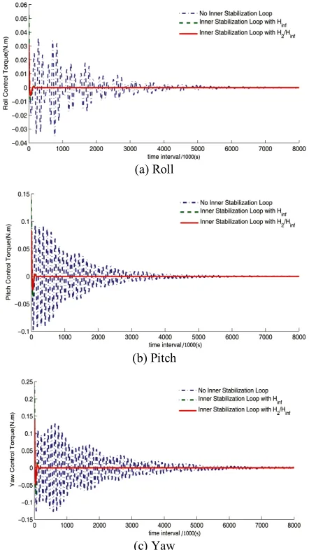
Figure 6. Channels control command comparison with and without GSP stabilizing

(9)

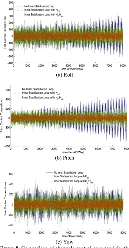
minimum control effort with maximum disturbance rejection, and the outer loop achieves the tracking objective with the help of error changes. The simulations show that this idea is very appropriate for the system and platform in tracking process to have an accurate stable situation. The tracking and control effort comparison are shown in Figures 6 and 7. Main characteristics of the proposed controller show its advantages which make it more preferable than the other controllers as to be optimal, and compensate disturbances and uncertainty of the system. So, to show these characteristics in controlled system with NLPID and proposed controller, a known disturbance has been exerted to system and with equal tracking trajectory, generated control moment to each channel are compared. It is shown that the exerted control moment to each channel with the use of integrated controller is lower than the same moment which is generated by the NLPID and a single sub-optimal _ℋ∞ controller.

(a) Roll

(b) Pitch

(c) Yaw

Figure 7. Implementation of integrated controller with platform stabilizing

(a) Roll

(b) Pitch

(c) Yaw

Figure 8. Comparison of channels control command for the implemented controllers with disturbance

7. CONCLUSION

The GSP has an oscillated line of sight, which complicates its control. The results show the effectiveness of the proposed controller in the presence of server disturbances to have a disturbance rejection and minimum power consumption at the same time.

8. REFERENCES

1. Pereira, G. J. and de Araujo, H. X., "Robust output feedback controller design via genetic algorithms and lmis: The mixed

H2/H∞ problem", in American Control Conference, IEEE. Vol. 4,

(2004), 3309-3314.

2. Apkarian, P., Noll, D. and Rondepierre, A., "Mixed H2/H∞

control via nonsmooth optimization", SIAM Journal on Control

(10)

3. Poussot-Vassal, C., Sename, O., Dugard, L., Gaspar, P., Szabo, Z., and Bokor, J., "Multi-objective qLPV H2/H∞ control of a half

vehicle", in Proceedings of the 10th Mini Conference on Vehicle System Dynamics, Identification and Anomalies, VSDIA. (2006).

4. Muradore, R. and Picci, G., "Mixed H2/H∞ control: The

discrete-time case", Systems & Control Letters, Vol. 54, No. 1, (2005), 1-13.

5. Popov, A., "Less conservative mixed H2/H∞ controller design

using multi-objective optimization", Technical University of

Hamburg, (2005).

6. Rotea, M. A. and Khargonekar, P. P., " H2-optimal control with

an H∞-constraint the state feedback case", Automatica, Vol. 27, No. 2, (1991), 307-316.

7. Erwin, R. S. and Bernstein, D. S., "Fixed-structure discrete-time

H2-optimal controller synthesis using the delta operator", in

American Control Conference, IEEE. Vol. 5, (1997), 3185-3189. 8. C., W. and Jr., R., "Direct reduced order mixed h2ih∞ control for the short take-off and landing maneuver technology demonstrator (stol/mtd)", Air Force Institute of Technology. (1994)

9. Scherer, C., "Mixed H2/H∞ control", Mechanical Engineering

Systems and Control Group Delft University of Technology. 10. Mut, V., Postigo, J., Carelli, R. and Kuchen, B., "Robust hybrid

motion-force control algorithm for robot manipulators",

International Journal of Engineering, Vol. 13, No. 4, (2000),

55-64.

11. Wang, Y. and Boyd, S., "Fast model predictive control using

online optimization", Control Systems Technology, IEEE

Transactions on, Vol. 18, No. 2, (2010), 267-278.

12. Raffo, G. V., Ortega, M. G. and Rubio, F. R., "An integral predictive/nonlinear H∞ control structure for a quadrotor helicopter", Automatica, Vol. 46, No. 1, (2010), 29-39.

13. De Caigny, J., Camino, J. F., Oliveira, R. C., Peres, P. L. D. and Swevers, J., "Gain-scheduled ℋ2 and ℋ∞ control of

discrete-time polytopic discrete-time-varying systems", IET Control Theory &

Applications, Vol. 4, No. 3, (2010), 362-380.

14. Camacho, E. F. and Bordons, C., "Model predictive control", Springer London, Vol. 2, (2004).

15. Kuhne, F., Lages, W. F. and da Silva Jr, J. M. G., "Point stabilization of mobile robots with nonlinear model predictive control", in Mechatronics and Automation, International Conference, IEEE. Vol. 3, (2005), 1163-1168.

16. Giovanini, L. L., "Predictive feedback control", ISA

Transactions, Vol. 42, No. 2, (2003), 207-226.

17. Mitsutomi, T., "Characteristics and stabilization of an inertial

platform", Aeronautical and Navigational Electronics, IRE

Transactions on, No. 2, (1958), 95-105.

18. Schaft, A. V. D. and Schaft, A., "L2-gain and passivity in

nonlinear control", Springer-Verlag New York, Inc., (1999). 19. Geromel, J. C., Peres, P. and Souza, S., "Convex analysis of

output feedback control problems: Robust stability and

performance", Automatic Control, IEEE Transactions on, Vol.

41, No. 7, (1996), 997-1003.

20. Scherer, C., Gahinet, P. and Chilali, M., "Multiobjective output-feedback control via lmi optimization", Automatic Control,

IEEE Transactions on, Vol. 42, No. 7, (1997), 896-911.

21. Ghany, A. M. A. and Alghmdi, A. G., Mixed H2/H∞ with

pole-placement design of robust lmi-based output feedback controller for a.C turbo-generator power system connected to infinite bus,

in 5th Saudi Technical Conference & Exhibition STCEX.:

Riyadh, Saudi Arabia, (2009)

22. Gahinet, P., Nemirovski, A., Laub, A. and Chilali, M., "MATLAB LMI control toolbox", The MathWorks Inc, (1995).