Capacitated Multimodal Structure of a Green Supply Chain Network Considering Multiple Objectives

(1)

International Journal of Engineering

J o u r n a l H o m e p a g e : w w w . i j e . i r

Capacitated Multimodal Structure of a Green Supply Chain Network Considering

Multiple Objectives

R. Sahraeian*, M. Bashiri, A. Taheri Moghadam

Department of Industrial Engineering, College of Engineering, Shahed University, Tehran, Iran

P A P E R I N F O

Paper history:

Received 21 November 2012 Received in revised form 08 April 2013 Accepted 16 May 2013

Keywords:

Green Supply Chain Network Design Multi-objective Optimization Multimodal Structure Normalized Normal Constraint Capacitated Transportation Network Non Dominated Sorting Genetic Algorithm-II

A B S T R A C T

In this paper, a supply chain network design problem is explained which contains environmental concerns in arcs and nodes of network. It is assumed that there are some routes such as road, rail, etc., in each pair of nodes. In this model decision variables are choosing facilities to open, environmental investment level in each facility and flow of products between nodes in each route. A multi-objective optimization model is proposed in this paper to capture the trade-off between the total cost and the environment influence. Some simulated numerical examples are considered to evaluate the model and the solution approach. Comparisons verify the suitability of the model and solution approach.

doi:10.5829/idosi.ije.2013.26.09c.04

1. INTRODUCTION 1

The field of green supply chain management (GSCM) has been attractive in recent years from both academia and industry. Nowadays, operations of supply chain and logistics are most important activities in companies. Production and transportation activities are main sources of air pollution and greenhouse effect, which have harmful effects on human health. These aspects have raised concerns for reducing greenhouse gas emission and air pollution. Many countries have set strict plans to reduce their carbon emissions. For example, china in its 11th five year developing plan sets a clear objective to reduce the carbon emission by 10 percent. [1]

Management of industrial pollution is a critical issue for society. During early periods, industrial pollution was not an interesting topic for researchers. In economics, taxes have been proposed to manage consequences such as industrial pollution [2]. However, the debate of taxing caused by industrial activities was essentially the limit of the discussions at the time. Some of the earliest issues that can be tied to the today's

*Corresponding Author Email:[email protected] (R.Sahraeian)

greening of the supply chain have occurred even before the formation of the U.S. Environmental Protection Agency, which can be traced to Ayres and Kneese [3]. Their work focused on a linear relationship from extraction to disposal; there were some loops concerning the possibility of integrating residues back into the system. Global warming due to greenhouse gas emissions was also going on the argumentation on evaluating the roles of industrial metabolism. Further refinement of the industrial metabolism ideas occurred throughout the 1970s [2]. Sadegheih et al. [4] proposed a model that concerns transportation problem connected with carbon emission. They have included carbon emission costs in the total cost of the supply chain.

(2)

which considers the setting up of some special facilities like recovery centers [11] or optimizing the network configurations in a closed-loop network [12]. In this paper we are interested in the environmental investment decision making in the network design phase. [1]

Another dependent field is the classical supply chain network design problem. It determines configuration parameters such as number, location, capacity, and type of various facilities in the network. This problem covers a wide range of formulations from linear deterministic models [13, 14] to complex non-linear stochastic ones [15, 16]. Numerous researches dealing with the design problem of supply networks have been surveyed by Pontrandolfo and Okogba [17]. Researchers have attempted to extend the classical model by incorporating various factors such as transportation modes, risk management, tax issue, etc. Wang et al. [1] have considered the environmental investment decision in the design phase and in this paper we combine their model by transportation modes.

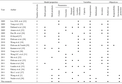
The supply chain network design problem is usually modeled as a single objective [18, 19]. Supply chain network design with multi-objective optimization is an influential trend worthy of study [1]. Adding transportation modes to Wang et al. [1] model would make it more reasonable and more practical in terms of actual applications. Some of recent studies in the field of green supply chain are briefly reviewed in Table 1. It shows that there are some potential fields to be studied. The distinguishing feature of our model is its consideration of environmental element which includes environmental level of facility and environmental influence in the handling and transportation process in different modes. This model will have an important application in the regional or global supply chain network design with environment consideration.

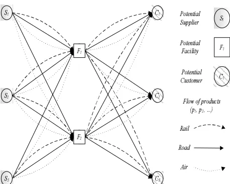
As it is mentioned in Table 1, multi modal models are not considered as well in green supply chain field. However, in real cases there are usually various mature modes of transportations like rail, road, air, sea or even electronic transportation; for example, in a book supply chain, distributors can sell electronic books instead of hard copies. Each mature transportation mode consists of different minor modes. For example, if decision maker choose road transportation, there are some other lower level choices like truck, mini-truck, van, motor cycle, bicycle, and so on. Each mature and minor mode has some advantages and disadvantages. For example, airplanes are fast, but they cannot be used for retailer’s activities and they have to mix with road transportation.

In this paper we proposed a multi-objective mixed-integer formulation for the supply chain network design problem, which considers the environmental investment decisions in the supply network design phase.

Normalized normal constraint method [20] is used for solving this model in small sizes, which is a prefered method and can find a set of non-dominated solutions.

For solving large size problems, NSGA-II method [21] is suggested, so that the results can be easily applied to the decision support systems which the industry needs.

The the paper has been organized as follows: section 2 describes assumptions and definition of the proposed model. In section 3, solution approach is explained. In section 4, the use of the proposed procedure is evaluated through computational experiments. Our concluding and suggestions for future researches are given in the final Section.

2. PROBLEM DEFINITION AND MODELING

The developed model contains two mature sets, N is the set of nodes and A is the set of arcs. N is composed by three levels, set of suppliers, S, facilities, F, and customers, C. There is at least one arc between nodes of one level to the next level (like road, rail, etc.), but there is no arc between nodes at the same level. Customers’ demand is supposed to be known. We should choose the potential suppliers from suppliers set; decide which facility to open, and finally how to distribute the products (flow of routes). There is two objectives; the first objective is minimizing total cost of the network, and the second is minimizing total CO2 emission of the whole network (plants and routes). The main difference between this model and that of Wang et al. [1] is considering modes of transportations (multi modal) and capacity of routes. In other words, the model prposed by Wang et al. [1] is a special case of the developed model, hence this model is more similar to real cases. Figure 1 represents the model. Parameters of this model are as follows:

Figure 1. The network consists of 3 suppliers, 2 facilities and

(3)

TABLE 1. Review of some existing models in green supply chain field.

Year Author

Model properties Variables Objectives

N

um

be

r

of

le

ve

ls

M

ulti

pe

ri

ods

M

ulti

pr

odu

cts Parameters

D

ema

nd

sa

tis

fac

tion

L

oca

tion

-A

llo

ca

tion

C

ap

ac

ity

T

ra

ns

po

rt

ati

on

M

ulti

m

od

al

Inv

en

to

ry

Pr

of

it/

C

ost

R

es

pon

si

bility

E

nv

ir

on

me

nt

pr

ot

ec

tion

C

er

ta

in

U

nce

rt

ain

2009 Lee, D.H. et al. [22] 4 ● ● ● ●

2009 Yang et al. [23] 6 ● ● ● ● ●

2009 Pokharel et al. [24] 5 ● ● ● ● ● ● ●

2009 Amaro et al. [25] 4 ● ● ● ● ●

2009 Pan Zh. et al. [26] 5 ● ● ● ● ● ● ●

2010 El-Sayed [27] 7 ● ● ● ● ●

2010 Pishvaee et al. [28] 5 ● ● ● ● ●

2010 Wang et al. [18] 6 ● ● ● ●

2010 Pishvaee & Torabi [29] 5 ● ● ● ● ● ● ●

2010 Kannan et al. [19] 6 ● ● ● ● ● ●

2010 Yang et al. [30] 4 ● ● ● ●

2010 Wang S.F. et al. [31] 5 ● ● ● ●

2011 Shi et al. [32] 4 ● ● ● ● ●

2011 Pishvaee et al. [33] 5 ● ● ● ● ● ●

2011 Kenne et al. [34] 7 ● ● ● ● ●

2011 Lundin et al. [35] 4 ● ● ● ● ● ●

2011 Paksoy et al. [36] 10 ● ● ● ●

2011 Wei J. et al. [37] 4 ● ● ● ●

2011 Wang et al. [1] 3 ● ● ● ● ● ●

2012 Nealer et al. [38] 2 ● ● ● ● ● ●

This research 3 ● ● ● ● ● ● ● ●

Parameters

P the set of products A the set of arcs S the set of suppliers F the set of facilities C the set of customers

M the set of routes existing between a pair of nodes

dip the demand of customer i for product p

sip the supply of supplier i for product p

cijmp transportation cost for product p from facility i

to facility j by mode m

Caijm the capacity of arc m between node i and j

fj setup cost for facility j

uj the production capacity in facility j

rjp capacities consumed by producing a unit of

product p in facility j

ljp production cost of product p in facility j

Decision variables 1,

0, j

if facility j is o pen y

otherw ise

ì = í î

xijmp the flow of product p from node i to node j at

route m

zj the environmental protection level in facility j

(4)

1

( )

1: min j j j( )j

j F j F

p p p p

ijm ijm j ijm

p P ij Am M p P j F i S m M

Obj µ f y g z

c x l x

Î Î

Î Î Î Î Î Î Î

= + +

+

å

å å å

åå å å

(1)

2

( )

2 : min p( ) p

j j ijm

j F p P i S m M p p

ijm ijm p P ij Am M

Obj µ w z x

e x

Î Î Î Î

Î Î Î

=

+

åå

å å

å å å

(2)

The first objective function measures total cost of whole supply chain network. The first term is the setup cost, the second term is the environmental investment, the third term is the total transportation cost and the last term is the total production cost. The second objective function measures the total CO2 emission in all the supply chain. The first term is the total CO2 emission by production activities in all facilities, and the second term denotes the total CO2 emission by transportation products at the network in all routes.

Constraints:

0

p p

ijm ijm

i S m M i C m M

x x j F p P

Î Î Î Î

- = " Î " Î

å å

(3)

p p

ijm j i F m M

x d j C p P

Î Î

= " Î " Î

å å

(4)

p p

ijm i i F m M

x s i S p P

Î Î

£ " Î " Î

å å

(5)

p p

j ijm j j

p P i S m M

r x u y j F

Î Î Î

£ " Î

å å å

(6)

p ijm ijm p P x Ca Î £

å

(7) j j

z £y L " Îj F (8)

( )

0 ,

p ijm

x ³ " i j Î " ÎA m M " Îp P (9)

{ }

0,1

j

y Î " Îj F (10)

[ ]

0,

j j

z ÎZ and z Î L " Îj F (11)

Constraint (3) ensures that inputs of the network are equal to outputs. Note that there is no inventory stored in the network because this model is a single period. Constraint (4) implies that the demand of all customers would be satisfied. Constraint (5) is suppliers' capacity constraint. Constraint (6) states that the total processing requirement of all products produced in facility j should not exceed the capacity of the facility, when it is opened and ensures that xijmp=0 when facility j is not opened (yj=0). Constraint (7) ensures that the flow of each route should not exceed the capacity of the route. If one route

has some physical or geographic conditions, its capacity can define it. For example, if there is no airline between two nodes, capacity of that route is zero. Constraint (8) indicates that only one environmental level can be chosen less than L for opening facility j. Constraints (9), (10) and (11) show that xijmp are non-negative, yj are binary variables, and zj are integers in interval [0, L]. The above model is an integer model and is not easy to solve [1]. For simplicity, some new variables are defied in next section to make it easier to solve.

3. SOLUTION APPROACH

First, due to the discrete and bounded property of zj, we introduce a series of binary variables. This action decreases solution complexity.

jl

1,

z

0,

if the environm ent protection level l is selected for facility j

otherw ise

ì ï

= _í

ï

î

Note that one and only one environmental protection level can be selected. Hence, the following property can be reached:

,

j jl jl j

l L l L

z z l where z y j F

Î Î

=

å

= " Î ₍₁₂₎

As the proof of this property we consider two cases. In the first case, the facility j is opened. Hence, yj=1. As one and only one environmental protection level is selected, therefore: 1 jl l L z Î =

å

.

Suppose that l is selected. Hence, the following term can be easily verified:

j jl jl

l L

z l z l z l

Î

= = =

å

In the second case, the facility j is closed, that is, yj=0. It follows that zjl=0 for all l, and then:

0

j jl

l L

z z l

Î

= =

å

.

As the summary of these two cases, we can conclude property is correct.

Then, gjl and wjlp can be defined as follows:

( )

jl j

g =g l " Îl L (13)

( )

p p

jl j

w

=

w

l

" Î

l

L

(14)

(5)

( , )

jl jl j

f =g +f " Îj F " Îl L

A new type of decision variable is defined, xjlp, which measures the amount of product p, produced in facility j at l environmental protection level.

p p

ijm jl

i F m l L

x x

Î Î

=

åå

å

(15)

Now we can introduce the modified model:

1

( )

min p p

ijm ijm jl jl p P ij A m M j F l L

p p

j jl p P j F l L

µ c x f z

l x

Î Î Î Î Î

Î Î Î

= +

+

å å å

åå

å å å

(16)

2

( )

m in p p

jl jl j F p P l L

p p ijm ijm p P ij A m M

µ w x

e x

Î Î Î

=

+

å å å

(17)

0

p p

ijm jim

i S m M i C m M

x x

j F p P

Î Î Î Î

- =

" Î " Î

å å

(18)

p p

ijm j i F m M

x d j C p P

Î Î

= " Î " Î

å å

(19)

p p

ijm i i F m M

x s i S p P

Î Î

£ " Î " Î

å å

(20)

p p j jl j jl p P

r x u z j F l L

Î

£ " Î " Î

å

(21)

( )

p ijm ijm p P

x Ca ij A m M

Î

£ " Î " Î

å

(22)

0

p p

ijm jl i F m M l L

x x j C p P

Î Î Î

- = " Î " Î

å å

å

(23)

1

jl l L

z j F

Î

£ " Î

å

(24)

( )

, 0 p p ijm jl x x

ij A p P l L

j F m M

³

" Î " Î " Î

" Î " Î

(25)

{ }

0,1

jl

z Î " Îj F " Îl L (26)

In the above formulation, constraints (18), (19), (20), and (22) are the same as before. Constraint (21) results from constraints (6) and (12). Constraint (23) is the same as Equation (5). Constraint (24) ensures that all facilities can be opened at only one environmental protection level. Constraints (25) and (26) define the variable types. It is well known that there exist multiple

non-dominated solutions for a multi-objective optimization problem, called pareto optimal. In this paper the normalized normal constraint method by messac et al. [20] is applied to solve the multi-objective model. This method can yield a well-distributed set of all available pareto solutions [1]. The basic idea is that we should first normalize the objectives, and install a new constraint to find the pareto solution in each step.

First of all, we should solve the modified model with each objective function separately and get the objective value µ1* and µ2* corresponding to first and second

objectives, respectively. After that, we normalize the two objectives by using the Equation (27). For each vector µ= [µ1(x) µ2(x)]T. the normalization design

matrix is as follows:

( )

( ) ( )

( )

( ) ( )

( )

1 2

1* 2*

1 1 2 2 2* 1* 1* 2*

1 1 2 2

[ ]

T

µ x µ x µ x

µ x µ x µ x µ x

=

é - - ù

ê ú = - -ê ú ë û (27) Hence;

( )

1*

[0,1]

µ x =

and

( )

2* _[1,0]

µ x =

To tune the steps of the pareto solutions we have a trade-off between the speed in solving the problem and the accuracy of the pareto solutions, where the more solution number k, causes the less speed but more accurate. Hence, we set k=30 and the step δ=1/(k -1)=1/29 which is a proper number of the point in the pareto solutions, and the model can be solved in a reasonable time. Given the weight 0≤αj≤1 that is used in each step for shift the added constraint by δ to find pareto solutions.

0,1 , , 1

j j j m

a = ´d = ¼ - (28)

We can generate the corresponding pareto points by solving the following sub-problem.

Sub-problem for jth point (j=0, 1, 2, …, m-1)

2 ( )

min=m x (29)

Subject to: Equation (18) - (26) ( ) ( )

1 x 2 x 2 j 1

m -m £ a - (30)

(6)

Figure 2. Performance of normalized normal constraint method for a two objective model.

Figure 3. Pareto solutions.

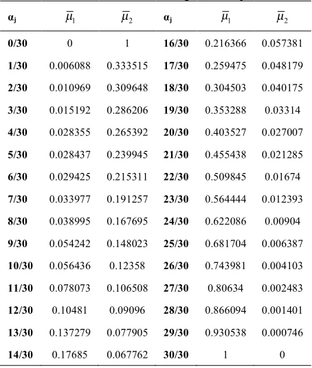
TABLE 2. Results of solving each sub-problem.

αj µ1 µ2 αj µ1 µ2

0/30 0 1 16/30 0.216366 0.057381

1/30 0.006088 0.333515 17/30 0.259475 0.048179

2/30 0.010969 0.309648 18/30 0.304503 0.040175

3/30 0.015192 0.286206 19/30 0.353288 0.03314

4/30 0.028355 0.265392 20/30 0.403527 0.027007

5/30 0.028437 0.239945 21/30 0.455438 0.021285

6/30 0.029425 0.215311 22/30 0.509845 0.01674

7/30 0.033977 0.191257 23/30 0.564444 0.012393

8/30 0.038995 0.167695 24/30 0.622086 0.00904

9/30 0.054242 0.148023 25/30 0.681704 0.006387

10/30 0.056436 0.12358 26/30 0.743981 0.004103

11/30 0.078073 0.106508 27/30 0.80634 0.002483

12/30 0.10481 0.09096 28/30 0.866094 0.001401

13/30 0.137279 0.077905 29/30 0.930538 0.000746

14/30 0.17685 0.067762 30/30 1 0

4. COMPUTATIONAL EXPERIMENTS

In this section we want to portrait a real scenario for demonstrating the solutions at first and after that we focused on the sensitivity analysis and its managerial insights. Finally, we have focused on the solution approach in different sizes. The problem is solved by GAMS 2.0.3.1 and MATLAB 2010a. All the experiments are conducted on a PC with Intel Core 2 Duo 2.40 GHz and 2 GB RAM. Although the data for the cases are randomly generated, they can nearly fit a real environment.

4. 1. Numerical Examples In this section an example is created by random data to evaluate the model and solution approach. The example is a mid-size network that has 11 nodes (5 customers, 3 facilities and 3 suppliers). Four environmental protection levels are assumed and there are 3 routes between each pair of nodes. The example is solved by GAMS 2.0.3.1 and the results are reported as follows.

The decision variables are (1) which facilities should be opened, and (2) which environmental protection level should be chose for opened facilities, (3) which suppliers should be selected, (4) the flow of products between suppliers, facilities and customers, (5) the flow of products at each route between nodes.

First, the modified model solved with first objective and µ1(x1*)=476.42 and µ2(x1*)=2827.4 is obtained. Then, the modified model solved with the second objective and µ1(x2*)=841.08 and µ2(x2*)=1747.9 is obtained. Now, we can normalize the objectives for using in normalized normal constraint method by Equation (27).

Therefore, k=30 sub-problems should be solved to obtain the pareto solutions. Each sub-problem is solved and the normalized pareto solutions are reported in Table 2. Note that normalized solutions should be at interval [0, 1] because the scale of objectives is removed by normalizing; hence, we can plot the normalized solutions at one diagram. Figure 3 shows the pareto solutions achieved in Table 2. Since the solver of GAMS cannot result the global optimum, a partial entropy is observed at j=4 and j=9.

For more clarification, solution of the example is shown in Figures 4 and 5. Figures 4 and 5 show the solutions corresponding to α=1 and α=0 respectively. In other words, Figure 4 shows optimal solution of second objective function and Figure 5 that of the first objective function. Note that in order to avoid complexity in figures, just the flow of first product is shown in Figures 4 and 5 and there are 5more products.

4. 2. Comparison with ε-Constraint Epsilon-constraint method is a useful method for finding pareto optimal line, which is used by many researchers [39]. In

0 0.2 0.4 0.6 0.8 1

Se

coned

ob

je

ct

iv

e:

CO

2

em

iss

ion

(7)

this section the numerical example is solved by ε -Constraint method with the same steps (α=30), and the results are reported in Figure 4. As it is shown in Figure 4, normalized normal constraint method is more accurate for finding pareto optimal line at the same step sizes. Hence normalized normal constraint approach is more efficient for solving this model.

Figure 4. Optimal flow of first product (α=1)

Figure 5. Optimal flow of first product (α=0)

Figure 6. Comparison with ε-Constraint

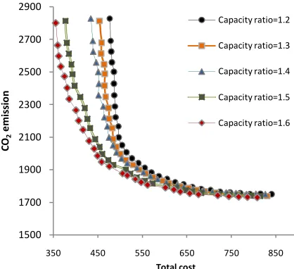
4. 3. Sensitivity Analysis We are interested in how capacity impacts the decision making. We define a “capacity ratio” which is the ratio of total network capacity over the total demands [1]. We vary this ratio from 1.2 to 1.6 and obtain a series of Pareto frontiers which are shown in Figure 7. It is clearly evident that the Pareto optimal curves move from right to left as the ratio increases from 1.2 to 1.6. It implies that, at the same CO2 emission level, larger capacity ratio leads to less total cost. While at the same total cost, CO2 emission is decreased by capacity ratio, as expected. In other words, supply chain network with larger capacity leads to lower total cost and lower CO2 emission. That is mainly because when the surplus capacity is installed, the network provides more flexibility to conduct the logistics such that the cost and the CO2 emission in the transportation process will reduce. The higher capacity may also provide possibilities that fewer facilities can be built and fixed costs will reduce. Note that the capacity is assumed external and given. In fact, it is possible that installing more capacity needs extra expense. Therefore, the decision maker can decide whether to improve the capacity of the network or not by examining this series of Pareto frontiers.

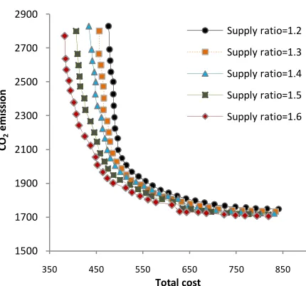
We are also interested in how supply impacts the decision making. We define a “supply ratio” that is the total network supply over the total demands. We vary this ratio from 1.2 to 1.6 and obtain a series of Pareto frontiers which are shown in Figure 8. It shows that when the supply ratio becomes larger, both CO2 emission and total cost will decrease. This tells us that increasing the supply can reduce both the CO2 emission and transportation cost becuase it is not necessary to get the products from a distant supplier. As a result, if possible, it is best for the decision maker to have the richer supply and closer to facilities in order to reduce the transportation CO2 emission and transportation cost.

Figure 7. Pareto optimal of different capacity ratio.

0 0.1 0.2 0.3 0.4 0.5 0.6 0.7 0.8 0.9 1

0 0.2 0.4 0.6 0.8 1

Se

cond

ob

je

ct

ive

: CO

2

em

issi

on

First objective: cost

EC NNC

1500 1700 1900 2100 2300 2500 2700 2900

350 450 550 650 750 850

CO2

em

issi

on

Total cost

Capacity ratio=1.2

Capacity ratio=1.3

Capacity ratio=1.4

Capacity ratio=1.5

(8)

Figure 8. Pareto optimal of different supply ratio.

4. 4. Evaluation Of The Model In Large Sizes In this section we evaluate the model in different sizes. As the objective of this study is to discover potential strategic managerial insights, we choose a mid-size sample for numerical examples because it is sufficient to represent its real supply chain network and it is computationally manageable. But, for evaluation of the efficiency of the model in large size problems, we compared GAMS results with "Non Dominated Sorting Genetic Algorithm-II" method (NSGA-II).

The proposed NSGA-II was first introduced by Deb et al. [21]. In the first step of NSGA-II algorithm, an initial population P0 is generated, randomly. In each

generation t, the following processes are carried out. All the offspring chromosomes Qt , the population of

children, are created with operations namely selection, crossover and mutation and they are evaluated.

Then, all the individuals from Pt and Qt are ranked

and they are placed in varying fronts. First Pareto front which is not dominated by other front is constituted and includes all the non-dominated solutions. In order to find the solutions in the next front, only the remaining solutions are considered. We repeat this process until ranking of all solutions are carried out and they are assigned to several fronts. After that, the best solutions, in the best front and with the most crowding distance, are selected for the new population Pt+1. This generation

is stopped if the stopping criterion is satisfied. The overall structure of the NSGA-II is as follows:

v Create the initial population P0 of size N v Estimate generated solutions

v Rank these solutions by non-domination and sort them by crowding distance

v While stopping criterion is not verified do

v Generate the offspring population Qt by selection, crossover and mutation

v Constitute the populations of parents and the children in Rt = Pt U Qt

v Sort the solutions of new population Rt in different

Pareto fronts Fi by the Pareto dominance v Pt+1 = 0

v i=1

v While |Pt+1|+|Fi|<Ndo

v Pt+1 = Pt+1 U Fi

v i=i+1

v End while

v Include in Pt+1, N − |Pt+1| solutions of Fi by

descending order of the crowding distance

v End while

In this paper, to solve NSGA-II, the number of population is set to 100, termination criterion is set to 100 and the crossover ratio is set to 1 with the possibility of 0.3. We set mutation probability equal to 0.45 and a mutation rate equal to 0.1. For mutation and crossover operations, we have used competitive method. The chromosomes in the proposed algorithm are defined as follows: [Obj1, Obj2, xijmp, zj]. The first and second

terms are the values of objective functions. The third term is the flow of products between each route; Note that yj (the opened facilities) will be defined by this

term. And the last term (zj) is environment protection

level in each open facility.

4. 4. 1 Quality of Solutions In this paper, we use different indexes to measure the performance of the algorithm such as the number of Pareto optimal solutions, quality of Pareto optimal solutions, CPU times, etc.

Uniform distribution of Pareto optimal solutions is the first index, which shows how close the Pareto optimal solutions are, and it is as follows:

(

)

2 1

1 1

n i i

S d d

n =

=

--

å

(31)

where n is the number of Pareto optimal solutions, di the distance to ith _{closest optimal solution which is}

calculated as follows,:

(

1 ( ) 1 ( ) 2( ) 2 ( )

)

min

i j i j

i j

d = f x -f x +f x -f x ₍₃₂₎ It is clear that smaller value of S represents better values.

1500 1700 1900 2100 2300 2500 2700 2900

350 450 550 650 750 850

CO

2

em

issi

on

Total cost

(9)

Quality of solutions is the second index. Let A and B be the quality of the solutions obtained by two algorithms. C(A,B) is defined as the ratio which is calculated as follows:

( , )

Number of solutions dominated by Solutions Number of solutions

C A B

B A

B =

(33)

Similarly we have:

( , )

Number of solutions dominated by Solutions Number of solutions

C B A

A B

A

=

(34)

And:

( , ) ( , )

C A B Q A B

C A B C B A

=

+ (35)

( , ) ( , )

C B A Q B A

C A B C B A =

+ (36)

( , ) ( , ) 1

Q A B +Q B A = (37)

It is obvious that better quality solutions are more desirable.

The other index is the diversity of the solutions, which can be calculated as follows:

2 , 1

( ) ( )

max

k k

i j k

D f i f j

=

å

- (38)

In Equation (38), i and j are the index of solutions and k is the index of the objective functions.

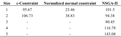
We have evaluated the algorithms in five different sizes which are introduced in Table 3. Each size is solved 30 times with random examples and the averages of the results are reported in Tables 4 to 8. The results show that for the small size problems GAMS performs accurate and fast. But for solving the medium and large sizes NSGA-II is suggested. Small size problems are solved with ε-constraint and NNC. Although ε -constraint is a little faster than NNC, but in the case of other indexes (such as number of pareto solutions, diversity of pareto solutions, and standard deviation of pareto solutions) NNC performs much better. Hence, according to the numerical examples, in small size problems NNC method is suggested and in medium and large sizes, the proposed NSGA-II can perform as well.

TABLE 3. The size of test problems

Test Problems 1 2 3 4 5

Customers 5 10 20 40 80

Facilities 3 8 16 32 64

Suppliers 3 6 12 24 48

Products 6 6 12 12 24

Environment investment levels 4 4 4 5 5

Routes 3 3 4 5 5

TABLE 4. Solution time.

Size ε-Constraint Normalized normal

constraint NSGA-II

1 1.46 2.09 61.42

2 28.41 28.72 191.14

3 Out of memory Out of memory 673.15 4 Out of memory Out of memory 2180.56 5 Out of memory Out of memory 10678.73

TABLE 5. The number of pareto solutions.

Size ε-Constraint Normalized normal constraint NSGA-II

1 30.87 30.93 52.02

2 30.83 30.87 44.37

3 - - 35.7

4 - - 28.70

5 - - 17.23

TABLE 6. The quality of pareto solutions.

Size Q (ε-Constraint, NNC) Q (NNC, NSGA-II)

Q (NSGA-II, NNC)

1 Divide by 0 1 0

2 Divide by 0 0.96 0.04

3 - - -

4 - - -

5 - - -

TABLE 7. The diversity of pareto solutions.

Size ε-Constraint Normalized normal constraint NSGA-II

1 1324.33 1337.2 1312.81

2 3150.32 3176.34 3157.1

3 - - 7022.51

4 - - 18355.33

5 - - 47180.74

TABLE 8. Standard deviation of the pareto solutions.

Size ε-Constraint Normalized normal constraint NSGA-II

1 95.67 23.46 101.5

2 106.73 38.83 94.38

3 - - 80.45

4 - - 116.78

5 - - 143.08

5. CONCLUSION

(10)

Normalized normal constraint method has been compared with ε-constraint for small size problems. The results showed that NNC is better than ε-constraint for achieving pareto solutions in small sizes. The small size problems are solved by GAMS 2.0.3.1 and for medium and large sizes we have suggested NSGA-II algorithm. The results show that this approach can obtain pareto solution in a reasonable time and the proposed model can be used in a real supply chains.

As a future research, one can consider a fuzzy approach for non-deterministic models. The reverse logistic can be applied in the same model or closing the loop of the network can be considered as some other areas for future studies.

6. REFERENCES

1. Wang, F., Lai, X. and Shi, N., "A multi-objective optimization for green supply chain network design", Decision Support

Systems, Vol. 51, No. 2, (2011), 262-269.

2. Sarkis, J., Zhu, Q. and Lai, K.-h., "An organizational theoretic review of green supply chain management literature",

International Journal of Production Economics, Vol. 130, No.

1, (2011), 1-15.

3. Ayres, R. U. and Kneese, A. V., "Production, consumption, and externalities", The American Economic Review, Vol. 59, No. 3, (1969), 282-297.

4. Sadegheih, A., Drake, P., Li, D. and Sribenjachot, S., "Global supply chain management under the carbon emission trading program using mixed integer programming and genetic algorithm", International Journal of Engineering,

Transactions B: Applications, Vol. 24, No., (2011), 37-53.

5. Srivastava, S. K., "Green supply_‐chain management: A state_‐of_‐the_‐art literature review", International Journal of

Management Reviews, Vol. 9, No. 1, (2007), 53-80.

6. Kuo, T.-C., Huang, S. H. and Zhang, H.-C., "Design for manufacture and design for ‘x’: Concepts, applications, and perspectives", Computers & Industrial Engineering, Vol. 41, No. 3, (2001), 241-260.

7. Sheu, J.-B., Chou, Y.-H. and Hu, C.-C., "An integrated logistics operational model for green-supply chain management", Transportation Research Part E: Logistics and Transportation

Review, Vol. 41, No. 4, (2005), 287-313.

8. Cheng, S., Chan, C. W. and Huang, G. H., "An integrated multi-criteria decision analysis and inexact mixed integer linear programming approach for solid waste management",

Engineering Applications of Artificial Intelligence, Vol. 16,

No. 5, (2003), 543-554.

9. Bloemhof-Ruwaard, J. M., Van Wassenhove, L. N., Gabel, H. L. and Weaver, P. M., "An environmental life cycle optimization model for the european pulp and paper industry", Omega, Vol. 24, No. 6, (1996), 615-629.

10. Zhu, Q., Sarkis, J. and Lai, K.-h., "Green supply chain management implications for “closing the loop”", Transportation Research Part E: Logistics and Transportation

Review, Vol. 44, No. 1, (2008), 1-18.

11. Fleischmann, M., Beullens, P., BLOEMHOF_‐RUWAARD, J. M. and WASSENHOVE, L. N., "The impact of product recovery on logistics network design", Production and

Operations Management, Vol. 10, No. 2, (2001), 156-173.

12. Savaskan, R. C., Bhattacharya, S. and Van Wassenhove, L. N., "Closed-loop supply chain models with product remanufacturing", Management Science, Vol. 50, No. 2, (2004), 239-252.

13. Melkote, S. and Daskin, M. S., "Capacitated facility location/network design problems", European Journal of

Operational Research, Vol. 129, No. 3, (2001), 481-495.

14. Romeijn, H. E., Shu, J. and Teo, C.-P., "Designing two-echelon supply networks", European Journal of Operational Research, Vol. 178, No. 2, (2007), 449-462.

15. Santoso, T., Ahmed, S., Goetschalckx, M. and Shapiro, A., "A stochastic programming approach for supply chain network design under uncertainty", European Journal of Operational

Research, Vol. 167, No. 1, (2005), 96-115.

16. Shu, J., Teo, C.-P. and Shen, Z.-J. M., "Stochastic transportation-inventory network design problem", Operations

Research, Vol. 53, No. 1, (2005), 48-60.

17. Pontrandolfo, P., "Global manufacturing: A review and a framework for planning in a global corporation", International

Journal of Production Research, Vol. 37, No. 1, (1999), 1-19.

18. Wang, H.-F. and Hsu, H.-W., "A closed-loop logistic model with a spanning-tree based genetic algorithm", Computers &

Operations Research, Vol. 37, No. 2, (2010), 376-389.

19. Kannan, G., Sasikumar, P. and Devika, K., "A genetic algorithm approach for solving a closed loop supply chain model: A case of battery recycling", Applied Mathematical Modelling, Vol. 34, No. 3, (2010), 655-670.

20. Messac, A., Ismail-Yahaya, A. and Mattson, C. A., "The normalized normal constraint method for generating the pareto frontier", Structural and Multidisciplinary Optimization, Vol. 25, No. 2, (2003), 86-98.

21. Deb, K., Pratap, A., Agarwal, S. and Meyarivan, T., "A fast and elitist multiobjective genetic algorithm: Nsga-ii", Evolutionary

Computation, IEEE Transactions on, Vol. 6, No. 2, (2002),

182-197.

22. Lee, D.-H. and Dong, M., "Dynamic network design for reverse logistics operations under uncertainty", Transportation

Research Part E: Logistics and Transportation Review, Vol.

45, No. 1, (2009), 61-71.

23. Yang, G.-f., Wang, Z.-p. and Li, X.-q., "The optimization of the closed-loop supply chain network", Transportation Research

Part E: Logistics and Transportation Review, Vol. 45, No. 1,

(2009), 16-28.

24. Pokharel, S. and Mutha, A., "Perspectives in reverse logistics: A review", Resources, Conservation and Recycling, Vol. 53, No. 4, (2009), 175-182.

25. Amaro, A. and Barbosa-Póvoa, A. P. F., "The effect of uncertainty on the optimal closed-loop supply chain planning under different partnerships structure", Computers & Chemical

Engineering, Vol. 33, No. 12, (2009), 2144-2158.

26. Pan, Z., Tang, J. and Liu, O., "Capacitated dynamic lot sizing problems in closed-loop supply chain", European Journal of

Operational Research, Vol. 198, No. 3, (2009), 810-821.

27. El-Sayed, M., Afia, N. and El-Kharbotly, A., "A stochastic model for forward–reverse logistics network design under risk",

Computers & Industrial Engineering, Vol. 58, No. 3, (2010),

423-431.

28. Pishvaee, M. S., Farahani, R. Z. and Dullaert, W., "A memetic algorithm for bi-objective integrated forward/reverse logistics network design", Computers & Operations Research, Vol. 37, No. 6, (2010), 1100-1112.

(11)

30. Yang, P., Wee, H., Chung, S. and Ho, P., "Sequential and global optimization for a closed-loop deteriorating inventory supply chain", Mathematical and Computer Modelling, Vol. 52, No. 1, (2010), 161-176.

31. Wang, H.-F. and Hsu, H.-W., "Resolution of an uncertain closed-loop logistics model: An application to fuzzy linear programs with risk analysis", Journal of Environmental

Management, Vol. 91, No. 11, (2010), 2148-2162.

32. Shi, J., Zhang, G. and Sha, J., "Optimal production planning for a multi-product closed loop system with uncertain demand and return", Computers & Operations Research, Vol. 38, No. 3, (2011), 641-650.

33. Pishvaee, M. S., Rabbani, M. and Torabi, S. A., "A robust optimization approach to closed-loop supply chain network design under uncertainty", Applied Mathematical Modelling, Vol. 35, No. 2, (2011), 637-649.

34. Kenne, J.-P., Dejax, P. and Gharbi, A., "Production planning of a hybrid manufacturing–remanufacturing system under uncertainty within a closed-loop supply chain", International

Journal of Production Economics, Vol. 135, No. 1, (2012),

81-93.

35. Lundin, J. F., "Redesigning a closed-loop supply chain exposed to risks", International Journal of Production Economics, Vol. 140, No. 2, (2012), 596-603.

36. Paksoy, T., Bektaş, T. and Özceylan, E., "Operational and environmental performance measures in a multi-product closed-loop supply chain", Transportation Research Part E: Logistics

and Transportation Review, Vol. 47, No. 4, (2011), 532-546.

37. Wei, J. and Zhao, J., "Pricing decisions with retail competition in a fuzzy closed-loop supply chain", Expert Systems with

Applications, Vol. 38, No. 9, (2011), 11209-11216.

38. Nealer, R., Matthews, H. S. and Hendrickson, C., "Assessing the energy and greenhouse gas emissions mitigation effectiveness of potential us modal freight policies", Transportation Research

Part A: Policy and Practice, Vol. 46, No. 3, (2012), 588-601.

(12)