The Effect of Added Mass Fluctuation on Heave Vibration of TLP

THE EFFECT OF ADDED MASS FLUCTUATION

ON HEAVE VIBRATION OF TLP

M. R. Tabeshpour, A. A. Golafshani

Department of Civil Engineering, Sharif University of Technology, Tehran, Iran [email protected], [email protected]

M. S. Seif

Department of Mechanical Engineering, Sharif University of Technology, Tehran, Iran [email protected]

(Received: July 16, 2004)

Abstract The resulting motion in waves can be considered as a superposition of the motion of the body in still water and the forces on the restrained body. In this study the effect of added mass fluctuation on vertical vibration of TLP in the case of vibration in still water for both free and forced vibration subjected to axial load at the top of the leg is presented. This effect is more important when the amplitude of vibration is large. Also this is important in fatigue life study of tethers. The structural model used here is very simple. Perturbation method is used to formulate and solve the problem. First and second order perturbations are used to solve the free and forced vibration respectively.

Key Words Added Mass Fluctuation, Wave, TLP, Heave Vibration, Perturbation Method

ﺪﻴﻜﭼ ﻩ

ﺯﺍﯽﺷﺎﻧﺖﮐﺮﺣﻭﻦﮐﺎﺳﺏﺁﺭﺩﻢﺴﺟﺖﮐﺮﺣﯽﻄﺧﺐﻴﮐﺮﺗﺕﺭﻮﺻﻪﺑﻥﺍﻮﺗﯽﻣﺍﺭﺝﻮﻣﺮﺛﺍﺮﺑﻩﺪﺷﺩﺎﺠﻳﺍﺖﮐﺮﺣ

ﺖﻓﺮﮔﺮﻈﻧﺭﺩﺖﺑﺎﺛﻢﺴﺟﻪﺑﻩﺩﺭﺍﻭﯼﺎﻫﻭﺮﻴﻧ

.

ﺭﺩ ﻦﻳﺍ ﻪﻌﻟﺎﻄﻣ ﺮﻴﻐﺘﻣﻩﺩﻭﺰﻓﺍﻡﺮﺟﺮﺛﺍ ﻦﮐﺎﺳﺏﺁﺖﻟﺎﺣﺭﺩ

ﺮﺑ ﻲﻜﻴﻣﺎﻨﻳﺩﺦﺳﺎﭘ ﻢﺋﺎﻗ

ﻭﺩﺍﺯﺁﺵﺎﻌﺗﺭﺍﺖﻟﺎﺣﻭﺩﻱﺍﺮﺑ،ﻲﺸﺸﻛﻪﻳﺎﭘﻱﺍﺭﺍﺩﻱﻮﻜﺳ ﺎﻌﺗﺭﺍ

ﺵ ﺖﺳﺍﻩﺪﺷﻪﺋﺍﺭﺍﻪﻳﺎﭘﻱﻻﺎﺑﺭﺩﻱﺭﻮﺤﻣﺭﺎﺑﺖﺤﺗﻱﺭﺎﺒﺟﺍ

.

ﻦﻳﺍ

ﺮﻣﺍ ،ﺪﺷﺎﺑﻱﺍﻪﻈﺣﻼﻣﻞﺑﺎﻗﺭﺍﺪﻘﻣﻱﺍﺭﺍﺩ،ﻩﺯﺎﺳﻢﺋﺎﻗﺵﺎﻌﺗﺭﺍﻪﻨﻣﺍﺩﻪﻛﻲﻄﻳﺍﺮﺷﺭﺩ ﻩﮋﻳﻮﺑ

ﺯﺍ ﺖﺳﺍﺭﺍﺩﺭﻮﺧﺮﺑﻱﺮﺘﺸﻴﺑﺖﻴﻤﻫﺍ

.

ﻦﻴﻨﭽﻤﻫ ﻦﻳﺍ ﺪﺷﺎﺑﻲﻣﺖﻴﻤﻫﺍﻱﺍﺭﺍﺩﺎﻬﻧﻭﺪﻧﺎﺗﻲﮕﺘﺴﺧﺮﻤﻋﻪﻌﻟﺎﻄﻣﺭﺩﺮﺛﺍ

.

ﺩﺭﻮﻣﻱﺍﻩﺯﺎﺳﻝﺪﻣ ﻩﺩﺎﻔﺘﺳﺍ

ﺪﺷﺎﺑﻲﻣﻩﺩﺎﺳﺭﺎﻴﺴﺑ

.

ﺵﺎﺸﺘﻏﺍﺵﻭﺭﺯﺍﻪﻟﺎﺴﻣﻞﺣﻭﻱﺪﻨﺑﻝﻮﻣﺮﻓﺭﻮﻈﻨﻣﻪﺑ ﻩﺩﺎﻔﺘﺳﺍ

ﺖﺳﺍﻩﺪﺷ

.

ﺭﺩ ﻪﺒﺗﺮﻣﻝﻼﺘﺧﺍﺯﺍ،ﺩﺍﺯﺁﺵﺎﻌﺗﺭﺍﺖﻟﺎﺣ ﻡﻭﺩ

ﺭﺩﻭ

ﺩﺭﻮﻣ ﺵﺎﻌﺗﺭﺍ ﻱﺭﺎﺒﺟﺍ ﺯﺍ ﺖﺳﺍﻩﺪﺷﻩﺩﺎﻔﺘﺳﺍﻝﻭﺍﻪﺒﺗﺮﻣﻝﻼﺘﺧﺍ

.

1. INTRODUCTION

Tension leg platforms (TLPs) are well-known structures for oil exploitation in deep water and are becoming increasingly popular for oil drilling at very deep water sites. Figure. (1) shows different components of the TLP made up of vertical and horizontal elements on the upper structure and vertical tendons connecting the structure to a foundation on the seabed. These structures consist of semi-submersible platforms with sufficient buoyancy to develop the required tension in the

basic component of the TLP. The most important point in the design of TLP is the pretension of the legs. The pretension causes that the platform behaves like a stiff structure with respect to the vertical degrees of freedom (heave, pitch and roll), whereas with respect to the horizontal degrees of freedom (surge, sway and yaw) it behaves as a floating structure. Therefore the periods of the vertical degrees of freedom are lower than the others. Among the various degrees of freedom, vertical motion (heave) is very important because of the direct effect on the stress fluctuation that leads to fatigue and fracture. Therefore the conceptual studies to understand the dynamic vertical response of TLP, can be useful for designers.

Simple models for heave response of tension leg platform under harmonic vertical load has been proposed [7]. The effect of added mass fluctuation on the heave response of tension leg platform has been investigated by using perturbation method for discrete [8] and continues model [9]. Added mass fluctuation has important effect on fatigue life of tethers [8].

In this study the effect of added mass fluctuation in the case of vibration in still water for both free and forced vibration is discussed. A similar formulation can be developed for motion analysis of the restrained body in waves. The problem is solved by means of perturbation method [10-11].

Figure 1. TLP configuration and components [12]

2. FREE VIBRATION ANALYSIS

The resulting motion in waves can be seen as a superposition of the motion of the body in still water and the forces on the restrained body in waves (Figure. 2).

Figure 2. Superposition of hydromechanical and wave loads [12]

In this paper the oscillation in still water is considered. Also in the case of small diameter, the forces of restrained body in waves are similar to the oscillation in still water. Structural modeling of a TLP as a moored structure is shown in Figure. (3). Free vibration equation of motion is as follows

0

= +ky y

m&& (1) where

) (t m m

m= s+ a (2) s

m is the structural mass and ma(t) is the time varying added mass, and

b

t k

k

k = + (3) where kt and kb are mooring and buoyancy stiffness respectively. If the structure is not being vertically moored, kt is equal to zero.

Total added mass can be considered as summation of two parts

) ( )

(t m0 m0y t

ma = a +ε a (4) where ma0 is constant and εma0y(t) is the time varying part. ε is the perturbation parameter and

) (t

y is the vertical motion. Defining a

m m

ma0/( s+ a0)= and ωn= k m 2

, the equation of motion can be written as

0 )

1

( +εay y&&+ω2ny= (5) Structural damping is assumed to be equal to zero. Perturbation method is used to solve the Eq. (5). A solution in the form of an infinite series of the perturbation parameter ε is assumed as follows

L + ε + ε + ε + = ( ) ( ) ( ) ( ) ) ( 3 3 2 2 1

0 t y t y t y t y

t

y (6)

The frequency of nonlinear vibration depends on the amplitude of vibration and perturbation parameter L + α ε + α ε + εα + ω =

ω 3 ₃

2 2 1 2 2

n (7)

where α_i are as yet undefined functions of amplitude. In this study, the second order perturbation method is used to solve the differential equation, therefore the response and frequency of vibration are considered as follows

) ( ) ( ) ( ) ( 2 2 1

0 t y t y t y

t

y = +ε +ε (8) 2

2 1 2

2 =ω +εα +ε α

ω n (9)

Substituting Eqs. (8) and (9) into Eq. (5), one obtains

[

]

{

}

[

]

[

( ) ( ) ( )

]

0

) ( ) ( ) ( ) ( ) ( ) ( ) ( 1 2 2 1 0 2 2 1 2 2 2 1 0 2 2 1 0 = ε + ε + × α ε − εα − ω + ε + ε + × ε + ε + ε + t y t y t y t y t y t y t y t y t y a && && && (10)

Since the perturbation parameter ε could have been chosen arbitrarily, the coefficients of the various powers of ε must be equated to zero. This leads to a system of equations which can be solved successively

0 0 2 0 +ω y =

y&& (11)

0 1 0 0 1 2

1 y ay y y

y_&& +ω =− _&& +α (12) 0 2 1 1 1 0 0 1 2 2

2 y a(y y y y) y y

y&& +ω =− && + && +α +α (13) The solution of the Eq. (11), subjected to the initial conditions y0(0)=A and y&0(0)=0, is

t A

y0 = cosω (14) Substituting Eq. (14) into the right hand side of the Eq. (12), one obtains

) 1 2 (cos 2 cos 2 2 1 1 2

1 ω +

ω + ω α = ω

+ y A t aA t

y&& (15)

The forcing term

cos

ω

t

leads to a secular term t

tcosω in the solution of y₁. Such terms violate the initial stipulation that the motion is to be periodic. Therefore one must impose the following condition

0 1 =

α (16) Now imposing the initial conditions

0 ) 0 ( ) 0 ( ₁

1 =y =

y & , the solution of the Eq. (15) is as follows ⎟ ⎠ ⎞ ⎜ ⎝

⎛ _{− ω − ω}

=aA t t

y cos2

3 1 cos 3 2 1 2 2

1 (17)

Substituting Eqs. (14) and (17) into Eq. (13), one obtains t A t t t t A a y y ω α + ⎟ ⎠ ⎞ ω ω ⎜ ⎝

⎛ _{ω − ω −}

ω = ω + cos 2 cos cos 3 5 cos 3 4 cos 2 2 2 2 3 2 2 2 2 && (18)

Equation (18) can be rewritten as

(

)

t A A a t t A a y y ω ⎟⎟ ⎠ ⎞ ⎜⎜ ⎝ ⎛ α + ω + ω + ω + × ω − = ω + cos 12 3 cos 5 2 cos 4 4 12 2 2 2 2 2 3 2 2 2 2 && (19) where 2 1 2 cos

2 3 cos cos 2 cos

cosωt ωt= ωt+ ωt have been used. Similarly the forcing term cosωt would lead to a secular term in the solution; therefore one must impose the following condition

12 2 2 2 2 ω − =

α a A (20) Now Eq. (19) becomes

(

t t

)

A a y y ω + ω + × ω − = ω + 3 cos 5 2 cos 4 4 12 2 3 2 2 2 2 && (21)

Imposing the initial conditionsy2(0)= y&2(0)=0, the solution of the Eq. (21) is as follows

(

)

t t t A a y ω + ω + ω + − = 3 cos 15 2 cos 32 cos 49 96 288 3 2

2 (22)

Substituting Eqs. (14), (17) and (22) into Eq. (8), the response of the system is obtained as follows

(

t t t

)

A a t t aA t A t y ω + ω + ω + − × ε + ⎟ ⎠ ⎞ ⎜ ⎝

⎛ _{− ω − ω}

ε + ω = 3 cos 15 2 cos 32 cos 49 96 288 2 cos 3 1 cos 3 2 1 2 cos ) ( 3 2 2 2 (23)

Substituting Eq. (20) into Eq. (7), the vibration frequency becomes 12 1 2 2 2 2 2 A a n ε + ω =

ω (24)

The frequency is found to decrease with the amplitude, as expected because of increasing in mass. Moreover considering the second order perturbation, the frequency ω decreases with the perturbation parameter. Therefore Eq. (23) is used to determine the response of the system with second order perturbation in which frequency ω is calculated from Eq. (24). First order perturbation response is determined from Eq. (23) in which

n

ω =

ω , and the terms having ε2

are vanished.

3. FORCED VIBRATION ANALYSIS

Forced vibration equation of motion is as follows

[

]

{

}

[

]

[

( ) ( ) ( )

]

cos( )

) ( ) ( ) ( ) ( ) ( ) ( ) ( 1 0 2 2 1 0 2 2 1 2 2 2 1 0 2 2 1 0 t m F t y t y t y t y t y t y t y t y t y a Ω = ε + ε + × α ε − εα − ω + ε + ε + × ε + ε + ε + && && && (25)

This leads to a system of equations which can be solved successively ) cos( 0 0 2 0 t m F y

y&& +ω = Ω (26) 0 1 0 0 1 2

1 y ay y y

y&& +ω =− && +α (27) 0 2 1 1 1 0 0 1 2 2

2 y a(y y y y) y y

y&& +ω =− && + && +α +α (28) The solution to the Eq. (26), subjected to the initial conditions 0y₀(0)= and y_&0(0)=0, is

2 2 0 0 ) cos( ) cos( Ω − ω Ω − ω −

= t t

m F

y (29)

Substituting Eq. (29) into the right side of the Eq. (27), one obtains

(

)

[

]

t t t t m F a t t m F y y Ω Ω − ω ω − − Ω + ω + Ω − ω Ω + ω × ⎟ ⎠ ⎞ ⎜ ⎝ ⎛ Ω − ω − Ω − ω Ω − ω α − = ω + 2 cos 2 cos 1 ) cos( ) cos( ) ( 2 ) cos( ) cos( 2 2 2 2 2 2 2 0 2 2 0 1 1 2 1 && (30)

Like previous one has 0

1=

α (16) The homogenous solution of Eq. (30) is

t C t C

y h = ω + ω

cos

sin ₂

1 ) (

1 (31) and the particular solution is

) 2 ( 2 2 2 2 2 2 0

1 _{Ω ω−Ω}

Ω + ω ⎟ ⎠ ⎞ ⎜ ⎝ ⎛ Ω − ω −

= a F m

D , ) 2 ( 2 2 2 2 2 2 0 2 Ω + ω Ω Ω + ω ⎟ ⎠ ⎞ ⎜ ⎝ ⎛ Ω − ω

=a F m

D , 2 2 2 0 3

6 ⎟⎠

⎞ ⎜ ⎝ ⎛ Ω − ω −

= a F m

D , 2 2 2 2 2 2 0 4 4

2 ω − Ω

Ω ⎟ ⎠ ⎞ ⎜ ⎝ ⎛ Ω − ω

=a F m

D , 2 2 2 2 2 2 0 5 2 ω Ω + ω ⎟ ⎠ ⎞ ⎜ ⎝ ⎛ Ω − ω

=a F m

D , C1=0,

) 4 )( 4 ( 6 11 4

3 2 2 2 2 2

6 4 2 2 4 6 2 2 2 0 2 Ω − ω Ω − ω ω Ω + Ω ω − Ω ω + ω ⎟ ⎠ ⎞ ⎜ ⎝ ⎛ Ω − ω −

= a F m

C

Now the solution of the Eq. (30) is as follows

⎭ ⎬ ⎫ ω Ω + ω − Ω Ω − ω Ω − ω + Ω + ω Ω + ω Ω Ω + ω − Ω − ω Ω − ω Ω Ω + ω + ⎩ ⎨ ⎧ ω Ω − ω Ω − ω ω Ω + Ω ω − Ω ω + ω ⎟ ⎠ ⎞ ⎜ ⎝ ⎛ Ω − ω − = 2 2 2 2 2 2 2 2 2 2 2 2 2 2 2 6 4 2 2 4 6 2 2 2 0 1 3 2 cos 4 3 2 cos ) cos( ) 2 ( 3 ) cos( ) 2 ( 3 cos ) 4 )( 4 ( 6 11 4 2 6 t t t t t m F a y (33)

Substituting Eqs. (29) and (33) into Eq. (28), one obtains 2 2 0 2 1 0 0 1 2 2 2 ) cos( ) cos( ) ( Ω − ω Ω − ω α − + − = ω + t t m F y y y y a y

y&& && &&

(34)

where

(

− ω + ω Ω − ω Ω + ω Ω − ω Ω + Ω

)

×

Ω ω − = + 10 8 2 6 4 4 6 2 8 10 2 3 3 0 1 0 0 1 4 29 67 67 29 4 6 5 m aF y y y y && &&

(

)

{

ω912cos(2ω+Ω)t−12cos(2ω−Ω)t−6cos(ω+2Ω)t+6cos(ω−2Ω)t +

+ ⎟⎟ ⎠ ⎞ ⎜⎜ ⎝ ⎛ Ω + ω − ω − Ω − ω + ω − − Ω − ω − Ω + Ω + ω + Ω − ω + Ω + ω + ω − Ω ω t t t t t t t t t t ) 2 cos( 9 cos 14 ) 2 cos( 22 3 cos 20 4 ) 2 cos( 9 cos 12 ) 2 cos( 22 ) cos( 2 ) cos( 2 2 cos 4 8

(

− ω− Ω + ω−Ω + ω+ Ω − ω+Ω

)

+

Ω

ω7 2 12cos( 2 )t 36cos(2 )t 12cos( 2 )t 36cos(2 )t

) 35 ( ) 2 cos( 45 cos 73 ) 2 cos( 85 3 cos 85 16 ) 2 cos( 45 cos 66 ) 2 cos( 85 ) cos( 10 ) cos( 10 2 cos 16 3 6 + ⎟⎟ ⎠ ⎞ ⎜⎜ ⎝ ⎛ Ω + ω + ω + Ω − ω − ω + − Ω − ω + Ω − Ω + ω − Ω − ω + Ω + ω + ω − Ω ω t t t t t t t t t t

(

− ω− Ω + ω−Ω + ω+ Ω − ω+Ω

)

+

Ω

ω5 4 42cos( 2 )t 48cos(2 )t 42cos( 2 )t 48cos(2 )t

+ ⎟⎟ ⎠ ⎞ ⎜⎜ ⎝ ⎛ Ω + ω + ω − Ω − ω − ω − − Ω − ω + Ω − Ω − Ω + ω − Ω − ω − Ω + ω − ω Ω ω t t t t t t t t t t t ) 2 cos( 63 cos 62 ) 2 cos( 16 3 cos 20 16 ) 2 cos( 63 3 cos 60 cos 12 ) 2 cos( 16 ) cos( 14 ) cos( 14 2 cos 44 5 4

(

− ω− Ω + ω+ Ω

)

+ Ω

ω3 6 24cos( 2 )t 24cos( 2 )t

+ ⎟⎟ ⎠ ⎞ ⎜⎜ ⎝ ⎛ Ω + ω − ω − Ω − ω + Ω − ω − Ω + Ω + Ω + ω + Ω − ω − Ω + ω − ω − − Ω ω t t t t t t t t t t ) 2 cos( 36 cos 24 ) 2 cos( 16 ) 2 cos( 36 3 cos 15 cos 117 ) 2 cos( 16 ) cos( 10 ) cos( 10 2 cos 24 24 7 2

(

12cos( )t 24cos t 12cos( )t

)

}

9 ω−Ω − Ω + ω+Ω

(

)

(

10 8 2 6 4 4 6 2 8 10

)

6 4 2 2 4 6 2 2 2 0 2 4 29 67 67 29 4 24 62 73 14 ) ( 6 5 Ω + Ω ω − Ω ω + Ω ω − Ω ω + ω − Ω − Ω ω − Ω ω + ω − Ω − ω ⎟ ⎠ ⎞ ⎜ ⎝ ⎛ = α m aF (36) and

(

)

(

10 8 2 6 4 4 6 2 8 10

)

6 4 2 2 4 6 2 2 2 0 2 2 2 4 29 67 67 29 4 24 62 73 14 ) ( 6 5 Ω + Ω ω − Ω ω + Ω ω − Ω ω + ω − Ω − Ω ω − Ω ω + ω − Ω − ω ⎟ ⎠ ⎞ ⎜ ⎝ ⎛ ε − ω = ω m aF

n (37)

Now the first order perturbation solution becomes

3 2 cos 4 3 2 cos ) cos( ) 2 ( 3 ) cos( ) 2 ( 3 cos ) 4 )( 4 ( 6 11 4 2 6 ) cos( ) cos( ) ( 2 2 2 2 2 2 2 2 2 2 2 2 2 2 2 6 4 2 2 4 6 2 2 2 0 2 2 0 ⎭ ⎬ ⎫ ω Ω + ω − Ω Ω − ω Ω − ω + Ω + ω Ω + ω Ω Ω + ω − Ω − ω Ω − ω Ω Ω + ω + ⎩ ⎨ ⎧ ω Ω − ω Ω − ω ω Ω + Ω ω − Ω ω + ω × ⎟ ⎠ ⎞ ⎜ ⎝ ⎛ Ω − ω ε − Ω − ω Ω − ω − = t t t t t m F a t t m F t y (38)

in which

ω

=

ω

n.

4. CASE STUDY

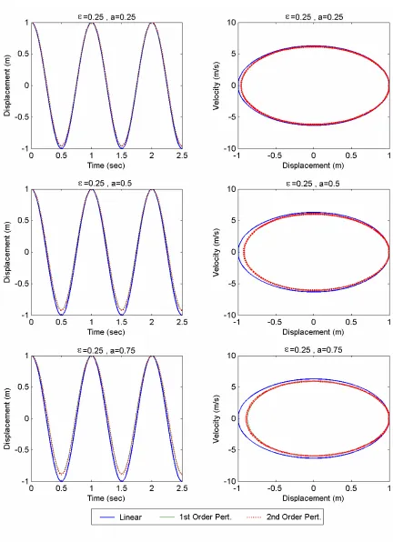
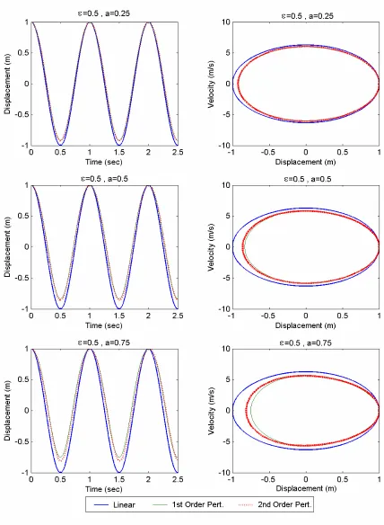
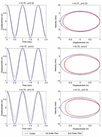
A numerical study has been carried out to understand the effect of parameters ε and a on the amplitude and frequency of vibration. It is supposed that the period of the structure is equal to 1, therefore the frequency of system is ω=2 , π and the initial condition A=1 is imposed. In Figures (4-6) the time histories and phase planes of system are shown for various values of ε and a. Figure. (4) shows the response time history phase plane for ε=0.25 and a= 0.25, 0.5 and 0.75. It is observed that the solution of first and second order perturbations are close together and for a= 0.25, 0.5 and 0.75, the differences between the amplitudes of the first and second order perturbations are 5%, 9% and 14% respectively. Similar results for ε=0.5 and ε=0.75 are obtained from Figures. (5) and (6). In the case of

5 . 0

=

ε the differences between the amplitudes related to various values of a are increased clearly. Also in the case of ε=0.75 the differences between the amplitudes related to various values of

a is more clear rather than previous values.

Phase planes illustrated in Figures (4-6) show the stability and periodicity of the solutions. The differences between the amplitudes related to various values of a are shown in other way.

It is seen that for small values of a, the difference between the first and second order perturbations is small and it increases with increasing a. Also increase in perturbation parameter ε, leads to increase the difference between linear response and both the first and second order perturbation solutions.

5. CONCLUSION

The effect of added mass fluctuation on the heave motion of a TLP subjected to axial load (or initial conditions) at the top of the leg has been investigated. Perturbation method has been used to formulate and solve the problem. The solution gives a conceptual view of the heave motion of a TLP, also it is important in fatigue life study of mooring lines. The parametric study shows the effect of some parameters on the response in the case of first and second order perturbation.

6. REFERENCES

1. Faltinsen, O. M., Van Hooff, R. W., Fylling, I. J., Teigen, P. S. "Theoretical and Experimental Investigations of Tension Leg Platform Behavior", Proceedings of BOSS 1, (1982), 411-423.

2. Siddiqui N. A., and Ahmad S., "Fatigue and Fracture Reliability of TLP Tethers under Random Loading", Journal of Marine Structures, Vol. 14, (2001), 331-352.

3. Teigen, P. S., "The Response of a Tension Leg Platform in Short-Crested Waves", Proceedings of the Offshore Technology Conference, OTC No. 4642, (1983), 525-532.

4. Jain, A. K., "Nonlinear Coupled Response of Offshore Tension Leg Platforms to Regular Wave Forces", Ocean Engineering, Vol. 24, No. 7, (1997), 577-592.

5. Ahmad S., "Stochastic TLP Response under Long Crested Random Sea", Journal of Computers and Structures, Vol. 61, No. 6, (1996), 975-993.

6. Chandrasekaran, S., Jain, A. K., "Nonlinear Dynamic Behaviour of Offshore Tension Leg Platforms under Regular Wave Lloads. Ocean Engineering Vol. 28, No. 12, (2001).

7. Tabeshpour, M.R., Golafshani, A.A., and Seif, M.S., "Simple Models for Heave Response of Tension Leg Platform under Harmonic Vertical Load", 8th International Conference of Mechanical Engineering, Tarbiat Modares University, (2004), Iran.

8. Tabeshpour, M.R., Golafshani, A.A., and Seif, M.S., "The Effect of Added Mass Fluctuation on Vertical Motion of Moored Sstructures" 8th International Conference of Mechanical Engineering, Tarbiat Modares University, Tehran, Iran, (2004), (in Farsi).

9. Tabeshpour, M. R., Seif, M. S. and Golafshani, A. A., "Vertical Response of TLP with the Effect of Added Mass Fluctuation", 16th Symposium on Theory and Practice of Shipbuilding, SORTA, (2004), Crovatia.

10. Nayfeh, A. H., Perturbation Methods, New York: John Wiley & Sons, (1973).

11. Kevorkian, J., and Cole, J. D., Perturbation Methods in Applied Mathematics, New York: Springer-Verlag, (1981).

12. Journee, J. M. J., and Massie, W. W., Offshore Hydromechanics, Delft University of Technology, (2001).