Modification of Sidelobe Canceller System In Planar Arrays (RESEARCH NOTE)

(1)

RESEARCH NOTE

MODIFICATION OF SIDELOBE CANCELLER SYSTEM

IN PLANAR ARRAYS

Nader Komjani*

Department of Electrical Engineering, Iran University of Science and Technology Tehran, Iran, [email protected]

Reza Mohammadkhani

Department of Electrical Engineering, University of Kurdistan Sanandaj, Iran, [email protected]

*Corresponding Author

(Received: March 7, 2004 - Accepted in Revised Form: February 4, 2006)

Abstract A Side Lobe Canceller (SLC) structure is a conventional partially adaptive technique which is used in large adaptive array radars. If a desired signal has long time duration in comparison with the SLC adaptation time, signal components may be cancelled. So, this paper presents a modified SLC which eliminates desired signal cancellation problems and allows using an unconstrained adaptive algorithm. Simulation results demonstrate the performance of this modified structure for a planar array.

Key Words Side Lobe Canceller, Generalized Side lobe Canceller, Adaptive Array, Planar Array

ﻩﺪﻴﻜﭼ

ﻭﻲﻫﺩ ﻞﻜﺷ

ﻘﻓ ﻣﻝﺎﻨﮕﻴﺳﻚﻳﻱﺍﺮﺑﻲﻜﻴﻨﻜﺗﻮﺗﺮﭘﻲ ﺎﺑﺎﻬﻠﺧﺍﺪﺗ ﻑﺬﺣﻭﻡﻮﻠﻌﻣ ﻱﺎﺘﺳﺍﺭﻚﻳ ﺯﺍﺏﻮﻠﻄ

ﺸﺗﻮﺗﺮﭘﻝﺮﺘﻨﻛ ﻘﻓﻭ ﺵﻭﺭﻚﻳﺎﺑﻱﺍ ﻪﻳﺍﺭﺁﻦﺘﻧﺁﻲﻌﺸﻌ

ﻲﻣﻲ ﺭﺎﺘﺧﺎﺳﺪﺷﺎﺑ

SLC

ﻱﺎﻫ ﺭﺎﺘﺧﺎﺳﻦﻳﺮﺗﺞﻳﺍﺭﺯﺍﻲﻜﻳ

ﺖﺳﺍﮒﺭﺰﺑﻱﺎﻫﻪﻳﺍﺭﺁﺵﺯﺍﺩﺮﭘﺭﺩﻲﻘﻓﻭﻩﺭﺎﭘ

.

ﺎﻤﻟﺍﺯﺍﻲﺧﺮﺑﺭﺎﺘﺧﺎﺳﻦﻳﺍﺭﺩ ﻲﻘﻓﻭﻝﺮﺘﻨﻛﻱﺍﺮﺑﺩﻮﺟﻮﻣﻪﻳﺍﺭﺁﻱﺎﻬﻧ

ﻪﺘﻓﺮﮔﺭﺎﻜﺑﻲﻘﻓﻭﺕﺎﻴﻠﻤﻋﻡﺎﺠﻧﺍﻭ ﻲﻣ

ﺩﻮﺷ

.

ﺎﻣﺍ ﻪﮐﯽﻣﺎﮕﻨﻫ ﺏﻮﻠﻄﻣﻝﺎﻨﮕﻴﺳ

ﺭﺎﺘﺧﺎﺳﻦﻳﺍﺭﺩ ﻲﮔﺭﺰﺑﺭﺎﻛﻩﺭﻭﺩﻱﺍﺭﺍﺩ

-ﺵﺯﺍﺩﺮﭘﻥﺎﻣﺯﺎﺑﻪﺴﻳﺎﻘﻣﺭﺩ

–

ﺪﺷﺎﺑ ،

ﻲﻣﻑﺬﺣﻲﺟﻭﺮﺧﺭﺩﺏﻮﻠﻄﻣﻝﺎﻨﮕﻴﺳﺯﺍﻲﺸﺨﺑ

ﺩﻮﺷ

.

ﻚﻳﻪﻟﺎﻘﻣﻦﻳﺍﺭﺩ

ﺭﺎﺘﺧﺎﺳ

SLC

ﺎﻬﻨﺸﻴﭘ ﻪﺘﻓﺎﻳ ﺩﻮﺒﻬﺑ ﻲﻣ ﺩ

ﻚﻳ ﺯﺍ ﻩﺩﺎﻔﺘﺳﺍ ﺎﺑ ﻪﻛ ﺩﻮﺷ ﺍ

ﻭ ﻢﺘﻳﺭﺎﮕﻟ ﻘﻓ

ﻝﺎﻨﮕﻴﺳ ﻑﺬﺣ ﻪﻠﺌﺴﻣ ﻲﻃﺮﺷ ﻲ

ﺪﻳﺎﻤﻧﻑﺮﻃﺮﺑﺍﺭﺏﻮﻠﻄﻣ

.

ﻱﺯﺎﺳﻪﻴﺒﺷﺞﻳﺎﺘﻧ ،

ﻲﻣﻥﺎﺸﻧﺍﺭﻪﺘﻓﺎﻳﺩﻮﺒﻬﺑﺭﺎﺘﺧﺎﺳﻦﻳﺍﻲﻳﺁﺭﺎﻛ ﺪﻫﺩ

.

1. INTRODUCTION

An adaptive beamformer is a processor used in conjunction with an array of sensors that is able to separate signals collocated in the frequency band but separated in the spatial domain [1]. This provides a means for separating a desired signal from interfering signals.

Adaptive beamforming started with the invention of the SLC (side lobe canceller) [2] in the latter of 1950’s. The fully adaptive array [3] was first conceived as a generalization of the side lobe canceller. A fully adaptive array with every element controllable provides theoretically the necessary side lobes to any arbitrary level.

In large fully adaptive arrays, high computational loads and low convergence speeds are two severe problems. For instance, large phased array radars possess thousands of elements, but practically it is only possible to process a few tens of adaptive degrees of freedom [4]. Hence, reducing adaptive dimension can reduce the system complexity and result in faster adaptive response [5-6]. SLC structure is used in large phased array radars as a partially adaptive technique [7,8].

(2)

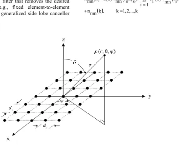
Figure 1. A planar array of N_xN_y elements located in xy plane. were commonly neglected. This was justified by

the usually valid assumption that the pulse signals reflected from targets of interest in the main beam were of sufficiently low power and/or duration that the control circuitry of the adaptive processor would not respond to them [9]. In more recent applications, high power and long-duration transmitted waveforms may cause to create a more serious signal cancellation problem [9].

A variety of approaches have been suggested for avoiding this problem in adaptive arrays [7-17]. These methods are categorized as:

1. Constrained Adaptive Algorithms

[10-12] In these approaches, some constraints are imposed directly in the adaption control loops. These techniques can be used in both fully and partially adaptive arrays.

2. Preadaption Spatial Filters

In this configuration, two beams are formed to applying constraints in an adaptive array. One beam has fixed weights (e.g., uniform, Chebyshev or Taylor) chosen to form the desired quiescent pattern. The second beam is formed by an adaptive processor following a spatial filter that removes the desired signal samples, e.g., fixed element-to-element subtraction [9], or generalized side lobe canceller

(GSC) [13]. These methods are used in fully adaptive arrays. More recent partially adaptive arrays based on GSC structure require an accurate estimation of an input data covariance matrix [14-17].

In this paper, we suggested a new approach to SLC systems in the planar arrays based on preadaption spatial filtering which create a null in the direction of the desired signal in the auxiliary channel (adaptive channel) to avoid signal cancellation. The proposed solution method follows the idea first introduced in [7,8]. Simulation results demonstrate the performance of this modified SLC structure.

2. FULLY ADAPTIVE ARRAY

For array beamforming with full adaptivity, we consider a planar array with N_x´ N_y elements shown in Figure 1. Let denote the received signal at mn th_{sensor, at}_k th_{time step as}

( ) ( )

( )

k, k 1,2,...,k mn

n

i

φ

, i

θ

mn v k i J D

1 i s

φ

, s

θ

mn v k S k mn x

= +

∑ = + =

(3)

Figure 2. GSC beamformer. where S( )k denotes the target signal, J k_i( ) is the

ith_{interference,} _{( )} mn

n k denotes the mnth_element

noise which is modeled as a zero-mean spatially white Gaussian random process, and v_mn

( )

θ,φ is expressed as

( )

θ,φ =exp

[

jωτ (θ,φ

]

v _mn (2)

where τ_mn

( )

θ,φ is the relation time delay of mnth

element to an arbitrary chosen spatial reference point. With respect to this reference point, mnth

element has location (xmn, ymn, zmn). The time delay

is given by

( )

/c

cos mn z sin sin mn y cos sin mn x , n

m _⎟⎟

⎠ ⎞ ⎜ ⎜ ⎝ ⎛ θ + φ θ + φ θ = φ θ

τ (3)

where c is the propagation speed of the incoming waves (signals). Define the NxNy dimensional

received vector x, array steering vector v

( )

θ,φ , and noise vector n as

( )

T k y N x N x ,..., k x , k x N x ,..., k x k ⎥ ⎥ ⎥ ⎦ ⎤ ⎢ ⎢ ⎢ ⎣ ⎡ = 12 1 11

x ₍₄₎

( )

T θ, y N x N v ,..., θ, v , θ, x N v ,..., θ, v φ θ, ⎥ ⎥ ⎥ ⎦ ⎤ ⎢ ⎢ ⎢ ⎣ ⎡ φ φ φ φ = 12 1 11

v ₍₅₎

( )

T k y N x N n ,..., k n , k x N n ,..., k n k ⎥ ⎥ ⎥ ⎦ ⎤ ⎢ ⎢ ⎢ ⎣ ⎡ = 12 1 11

n (6)

using 1-6, we can express x as

( ) ( )

(

)

( )

k ..., 2, , 1 = + φ ∑ = + φ = k , k i , i θ k i J D 1 i s , s θ k s

k v v n

x

(7)

in narrowband beamforming, a complex weight is applied to the signal at each sensor and sum to form the beamformer output

( )

k wH x

( )

k

y = (8)

where H denotes conjugate transpose, and w is

defined as

[

Nx NxNy

]

H

w

,...,

w

,

w

,...,

w

12 1 11

=

w

₍₉₎

The optimal weight vector w is found by

minimizing the array output power subject to L

linear or derivative constraints as follows

f w H C to subject w x R H w w

min = (10)

where ₌ _E

{

( )_k H( )_k

}

x

R x x is the data

covariance matrix, C is the Nx Ny ×L constraint

matrix, and f is the L×1 vector of constraint values.

The optimal solution is

(

C

R

C

)

f.

C

R

w

=

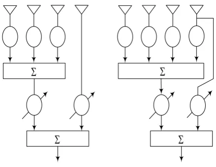
-1_x H -1_x −1 (11)

The GSC, shown in Figure 2, is a widely used beamforming structure that allows an unconstrained adaptive algorithm to be implemented to solve the constrained optimization problem [12]. wq is the NxNy dimensional

quiescent weight vector, B is the Nx Ny ×(Nx Ny – L)

signal blocking matrix where is orthogonal to C,

i.e. H ₌

B C 0 (see Appendix of [17]), and wa is the

(4)

Σ

Figure 3. Different types of SLC. .

q w x R H B 1 B x R H B a

w _⎟−

⎠ ⎞ ⎜

⎝ ⎛

= (12)

Let y ( )q ( )

H q

k = w x k and z( )k = B xH ( )k denote the outputs of the quiescent portion of the beamformer and the signal blocking matrix, respectively. The adaptive weights can be expressed as

z p -1 z R a

w = (13)

where ₌ H

z x

R B R B is the (Nx Ny – L)×(Nx Ny – L) covariance matrix of z( )k , and

H q

=

z x

p B R w is the (N – L)×1 cross-correlation

vector of z( )k and yq( )k .

3. SLC SYSTEM

Large radar arrays contain thousands of elements. Furthermore, digital hardware technology is rapidly advancing to the stage where huge element digitized arrays will be a reality. However, the difficulties of performing adaptive processing with such huge numbers of degree of freedom are well known [4]. Thus, partially adaptive processing techniques are used to reduce adaptive dimensions from thousands into a few tens of spatial degrees of freedom.

The SLC structure is a partially adaptive array, which can be used in two different forms [4] as shown in Figure 3. The conceptual scheme of an SLC system is shown in Figure 4. It consists of a non-adaptive phased-array that is called the main antenna, and an auxiliary array contains of a few controllable elements. The auxiliary antennas may be separate antennas or groups of receiving elements of a phased array antenna.

The purpose of the auxiliaries is to provide a replica of jamming signals in the sidelobes of the main pattern for cancellation. To this end the auxiliary patterns approximate the average sidelobe level of the main antenna receiving pattern [3]. The auxiliary antennas are placed sufficiently close to the phase center of the main

antenna to ensure that the samples of the interference that are obtained may be correlated with the interference received in the main antenna sidelobes. Also note that the number of auxiliary antennas must at least equal the jamming signals to be suppressed [18].

In conventional SLC, to prevent target-signal cancellation, its time duration is assumed to be much smaller than the SLC adaptation time. The amount of desired target signal received by the auxiliaries is also assumed to be negligible compared to the target signal in the main channel. Then, the target signal will pass unchanged through the SLC, while the jammer, which is continuous in time, will be reduced by the adaptation process operated by the canceller [3], [18].

(5)

Figure 4. Conventional SLC.

Figure 5. Modified SLC.

(

θ_s,φ_s

)

0 a

v H a

w = (14)

where H a

w is the adaptive weight vector of auxiliary array, and va

(

θs,φ_s

)

is the auxiliary array

steering vector along the target-signal direction. Define a blocking matrix as

H a v 1 a v H a v a v I

B= − ⎜_⎝⎛ ⎟_⎠⎞− (15)

where v_a =v_a

(

θ_s,φ_s

)

and B is orthogonal to

v

_a, i.e., H _a

(

θ_s,φ_s

)

=0

v

B . Received data vector of auxiliary array can be expressed as

[

1 2

]

( )

k

x k x k

( ), ( ), ,

x k

_M

( )

T

x

=

K

(16)

using blocking matrix B, as shown in Figure 5,

input data vector of adaptive processor is given by

( )

k B x

( )

k

x_a = H (17)

This input data vector contains just only interferences and noise components, therefore the adaptive processor can only suppress the interferences and noise signals, with independency of the target signal from other signals. In this structure, any unconstrained adaptive algorithm can be used.

4. SIMULATION RESULTS

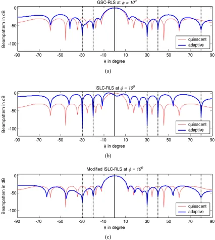
In this section, several simulation results are presented for illustration and comparison of the performance of a modified SLC for a planar array. We consider a planar array with 14x14 elements and half wavelength element spacing. Quiescent array elements are weighted with 30 dB Dolph-Chebyshev coefficients. The environment consists of a desired signal of power 0 dB, from the look

direction ₀o_, ₁₀o s s = φ =

θ and five jammers with powers 30 dB, 20 dB, 30 dB , 20 dB, and 20dB

from

, 10 , 30 ₁

1=− o φ = o

θ

, 10 , 20 ₂

2 =− o φ = o

θ

, 10 , 30 ₃

3= o φ = o

θ

, 10 , 40 ₄

4 = o φ = o

θ

, 10 , 80 5 5= o φ = o

θ respectively.

(6)

-90 -70 -50 -30 -10 10 30 50 70 90 -100

-50 0

θ in degree

B

ea

m

pa

tte

rn

in

d

B

GSC-RLS at φ = 10o

quiescent adaptive

(a)

-90 -70 -50 -30 -10 10 30 50 70 90

-100 -50 0

θ in degree

B

eam

pat

te

rn

in

dB

ISLC-RLS at φ = 10o

quiescent adaptive

(b)

-90 -70 -50 -30 -10 10 30 50 70 90

-100 -50 0

θ in degree

B

eam

pa

tt

er

n i

n

dB

Modified ISLC-RLS at φ = 10o

quiescent adaptive

(c)

Figure 6. Azimuth cut at f =10o of (a) fully adaptive GSC-RLS beampattern, (b) conventional Internal SLC-RLS beampattern and (c) modified Internal SLC-RLS beampattern.

be auxiliary elements, i.e., totally 12 auxiliary elements. Considering the slow convergence speed of LMS algorithm, RLS algorithm has been used. Figure 6(a) shows the beampattern of the fully adaptive GSC beamformer using a RLS adaptive algorithm. This beamformer maintains the unit gain in the direction of the desired signal and

(7)

0 100 200 300 400 500 600 700 800 900 1000 -4

-2 0 2 4

Sample number

am

pl

itude

Output of Quiescent array

(a)

0 100 200 300 400 500 600 700 800 900 1000

-1 -0.5 0 0.5 1 1.5

Sample number GSC-RLS output

S(k) y_out(k)

am

pl

itud

e

(b)

0 100 200 300 400 500 600 700 800 900 1000

-1 -0.5 0 0.5 1 1.5

Sample number ISLC-RLS output

S(k) y_out(k)

am

pl

itude

(c)

0 100 200 300 400 500 600 700 800 900 1000

-1 -0.5 0 0.5 1 1.5

Sample number Modified ISLC-RLS output

S(k) y_out(k)

(d)

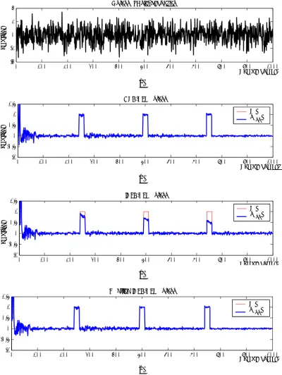
Figure 7. (a) Quiescent (non-adaptive) array output, (b) GSC-RLS output, (c) conventional Internal SLC-RLS output and (d) modified Internal SLC-RLS output.

Figure 7(a) shows the output of quiescent array that consists of a pulsive desired signal, five jammers and additive noise which are modeled as random processes. Outputs of fully adaptive GSC and conventional SLC are shown in Figures 7(b)

(8)

5. CONCLUSION

Conventional SLC systems in large phased arrays, cancel desired signals as well as undesired interferences. This paper suggested a new approach to combat this problem. The proposed technique imposes a null constraint in auxiliary array in the direction of the desiredsignal, and so eliminates undesirable effects of target signal cancellation phenomenon. This modified structure allows using an unconstrained adaptive algorithm. Several simulation results are shown to demonstrate the performance of this modified SLC in comparison with GSC and conventional SLC in a planar array

6. REFERENCES

1. VanVeen, B. D. and Buckley, K. M., "Beamforming: a versatile approach to spatial filtering", IEEE ASSP Magazine, (April 1988), 4-24.

2. Howells, P. W., "Intermediate frequency side-lobe canceller", U. S. Patent No. 3,202,990, (August 24, 1965 filed May 4, 1959).

3. Applebaum, S. P., "Adaptive arrays", IEEE Trans.

Antennas Propagat, Vol. AP-24, (September 1976),

573-598.

4. Zatman, M., "Degree of freedom architectures for large adaptive arrays", Asilomar Conference on Signals, Systems and Computers, (1999), 109-112.

5. Chapman, D. J., "Partial Adaptivity for the Large Array", IEEE Transactions on Antennas and Propagation, Vol. AP-24, No. 5, (September 1976). 6. Morgan, D. R., "Partially adaptive array techniques",

IEEE Trans. Antennas Propagat, Vol. AP-26,

(November 1978), 823-833.

7. Mohammadkhani, R., "Sidelobe Interference Suppression

in Fully and Partially Adaptive Array Radars”, MSc Thesis, Iran University of Science and Technology, (March 2004).

8. Komjani, N. and Mohammadkhani, R., "Sidelobe interference suppression in fully and partially adaptive array radars", Proceeding of 12th Iranian Conference of Electrical Engineering, Vol. 1, (May 2004), 599-604.

9. Applebaum, S. P. and Chapman, B. J., "Adaptive Arrays with Main Beam Constraints", IEEE Trans. On Antennas and Propagation, Vol. 24, (September 1976), 650-662.

10. Frost, O. L., "An Algorithm for Linearly Constrained Adaptive Array Processing", Proc. IEEE, Vol. 60, No. 8, (August 1972), 926-935.

11. Resende, L. S., Romano, J. M. T. and Bellanger, M. G., "A Robust FLS Algorithm for Linearly-Constrained Adaptive Filtering", Proc. ICASSP, Adelaide, Australia, (April 1994), 381-384.

12. Cheng, Y. H. and Chiang, C. T., "Adaptive beamforming using the constrained Kalman filter", IEEE Trans. Antennas and Propagation, Vol. 41, No. 11, (November 1993), 1576-1580.

13. Griffiths, L. J. and Jim, C. W., "An alternative approach to linearly constrained adaptive Beamforming", IEEE Trans. Antennas Propagat,Vol. 30, (January 1982), 27–34.

14. VanVeen, B. D., "Partially adaptive beamformer design via output power minimization", IEEE Trans. Acust., Speech, Signal Processing, Vol. 36, No. 3, (March 1988), 357-362.

15. VanVeen, B. D., "Eigenstructure based partially adaptive array design", IEEE Trans. Antennas and Propagation, Vol. 36, No. 3, (March 1988), 357-362. 16. Goldstein, J. and Reed, I., "Theory of partially adaptive

sensor array processing", IEEE Transactions on Signal Processing, Vol. 33, (April 1997), 539-544.

17. Goldstein, J. and Reed, I., "Theory of partially adaptive radar", IEEE Transactions on Aerospace and Electronic Systems, Vol. 33, (October 1997), 1309-1325.