SOLVING A BI-OBJECTIVE MANPOWER SCHEDULING
PROBLEM CONSIDERING THE UTILITY OF OBJECTIVE
FUNCTIONS
P.Shahnazari-Shahrezaei
Tehran, Iran
Department of Industrial Engineering, College of Engineering, University of Tehran, Tehran, Iran
Tehran, Iran [email protected]
*Corresponding Author
(Received: March 1, 2010 – Accepted in Revised Form: September 15, 2011)
doi: 10.5829/idosi.ije.2011.24.03b.05
Abstract This paper presents a novel bi-objective manpower scheduling problem that minimizes the penalty incurred by the employees’ assignment at lower skill levels than their real skills and maximizes the employees’ utility by assigning them at desired skill levels in some shifts/days. Employees are classified in two specialist groups and three skill levels in each specialization. In addition, the presented model executes some essential work regulations. This paper also proposes a solution procedure based on the utility of objective values. Applying this procedure, an effective point is obtained for the given problem. This is the point where both objective functions have the highest utility simultaneously.
Keywords Manpower Scheduling, Workforce Scheduling, Utility, Bi-objective Model
1. INTRODUCTION
Production factors are the economic resources which are used to produce goods and services. One
of the most important factors among them is the workforce or manpower. The work division which makes the highest possible efficiency of manpower is called “the proper allocation of human
H. Kazemipoor
.ﺪﻨﺷﺎﺑﻲﻣﻥﺎﻣﺰﻤﻫﺭﻮﻄﺑﺖﻴﺑﻮﻠﻄﻣﻦﻳﺮﺗﻻﺎﺑﻱﺍﺭﺍﺩﻑﺪﻫﻊﺑﺎﺗﻭﺩﺮﻫ ﻥﺁﺭﺩﻪﮐﺖﺳﺍﻱﺍﻪﻄﻘﻧﻥﺎﻤﻫﻦﻳﺍﻭﺪﻳﺁﻲﻣﺖﺳﺪﺑﻩﺪﺷﻪﺋﺍﺭﺍﻝﺪﻣﻱﺍﺮﺑﺮﺛﻮﻣﻪﻄﻘﻧﮏﻳ،ﻪﻳﻭﺭﻦﻳﺍﺯﺍﻩﺩﺎﻔﺘﺳﺍﺎﺑ .ﺩﻮﺷﻲﻣ ﺩﺎﻬﻨﺸﻴﭘﻑﺪﻫﺮﻳﺩﺎﻘﻣﺖﻴﺑﻮﻠﻄﻣﺮﺑﻲﻨﺘﺒﻣﻞﺣﻪﻳﻭﺭﮏﻳ،ﻪﻟﺎﻘﻣﻦﻳﺍﺭﺩﻦﻴﻨﭽﻤﻫ .ﺪﻨﮐﻲﻣﺍﺮﺟﺍﺍﺭﻱﺭﻭﺮﺿﻱﺭﺎﮐﺪﻋﺍﻮﻗ ﺯﺍﻲﺧﺮﺑ ﻩﺪﺷﻪﺋﺍﺭﺍﻝﺪﻣ،ﻦﻳﺍﺮﺑﻩﻭﻼﻋ .ﺪﻧﻮﺷﻲﻣﻱﺪﻨﺑﻪﻘﺒﻃﺺﺼﺨﺗﺮﻫ ﺭﺩﺕﺭﺎﻬﻣﺢﻄﺳﻪﺳﻭﺺﺼﺨﺘﻣﻩﻭﺮﮔﻭﺩ ﻪﺑﻥﺎﻨﮐﺭﺎﮐ .ﺖﺳﺍ،ﺪﻧﺭﺍﺩﺎﻫﺯﻭﺭﺎﻳﺎﻫﺖﻔﻴﺷﺯﺍﻲﺧﺮﺑﺭﺩﺹﺎﺧﺕﺭﺎﻬﻣﺢﻄﺳﮏﻳﺭﺩﻥﺩﺮﮐﺭﺎﮐﻪﺑﻞﻳﺎﻤﺗﻪﮐ ﻲﻧﺎﻨﮐﺭﺎﮐ ﺖﻴﺑﻮﻠﻄﻣ ﻥﺩﻮﻤﻧ ﺮﺜﮐﺍﺪﺣ ﻭﻥﺎﺷﻲﻌﻗﺍﻭ ﺕﺭﺎﻬﻣ ﺯﺍ ﺮﺗﻦﻴﺋﺎﭘ ﺕﺭﺎﻬﻣ ﺡﻮﻄﺳ ﺭﺩ ﻥﺎﻨﮐﺭﺎﮐ ﺺﻴﺼﺨﺗ ﺯﺍ ﻞﺻﺎﺣ ﻪﻤﻳﺮﺟ ﻥﺩﺮﮐﻞﻗﺍﺪﺣﻥﺁﻑﺪﻫﻪﮐﺪﻳﺎﻤﻧﻲﻣﻪﺋﺍﺭﺍﺍﺭﺪﻳﺪﺟﻑﺪﻫﻭﺩﻲﻧﺎﺴﻧﺍﻱﻭﺮﻴﻧﻱﺪﻨﺒﻧﺎﻣﺯﻪﻟﺎﺴﻣﮏﻳ،ﻪﻟﺎﻘﻣﻦﻳﺍ ﻩﺪﻴﻜﭼ
Department of Industrial Engineering, Parand Branch, Islamic Azad University Department of Industrial Engineering, Science and Research Branch, Islamic Azad University
*
resources”. Manpower should be scheduled to attain the proper allocation. Manpower scheduling is a managerial process that contains the analysis of human resources requirement of an organization in variable situations. It makes clear the policies and systems, which satisfy these requirements. The ultimate goal of manpower scheduling is to seek the shift rosters that conform to time-varying demand, so that it controls the costs and satisfies all executive regulations [1]. Since 1970’s manpower scheduling has allotted a broad field of research to itself. Apart from the scope of automated operations, all organizations such as: service companies, production companies, etc require manpower. As a general rule, manpower scheduling can be modeled in three categories: a) individual scheduling (e.g., nurse, physician, surgery and the like), b) group scheduling (e.g., crew), and c) personnel scheduling.
Manpower scheduling methods are usually divided into two approaches: cyclic and non-cyclic approaches [2]. Cyclic approaches are defined by fixed series of shifts that are approximately assigned to employees in an equal manner. Non-cyclic methods are generally placed on two groups: 1) the methods which are based on human’s experience and the spreadsheets, and 2) optimization methods that can be computerized entirely without so much necessity to human’s interference. In case of proper design, the latter will be capable to execute many rules concurrently. A matter at hand in manpower scheduling is workforce homogeneity or heterogeneity [3]. Homogeneous workforces are those whose available time is equal and necessity to them remains constant during a shift. Most full-time employees in production industries are placed on this group. Heterogeneous workforce is applied to those whose available time is different or necessity to them varies during a shift. Heterogeneous manpower scheduling is also called tour scheduling.
Manpower planning not only handles manpower scheduling but also deals with flexible working agreements. Some investigations on this subject are categorized to single-shift scheduling and multiple-shift scheduling [4-13]. In multiple-multiple-shift scheduling, each day is divided into several shifts, and scheduling determines which days of planning horizon and which hours of the day each employee is fitted to work.
manpower scheduling and finally suggested some points for the future research. Ingolfsson et al. [32] integrated queuing theory and cost minimization to model the random arrival process and the congestion that comes from a special schedule. Most manpower scheduling models usually deal with full-time personnel and part-time employees play the role of supplemental workforce in them. Glover et al. [33] presented a heuristic established upon Tabu search to produce the schedules for full-time workforce accompanied by part-full-timers. Willis et al. [34] used an integer programming approach for a staff scheduling problem in a call center containing both part-time and full-time staff. Schindler et al. [35] took a workforce problem at Pan American World Airways into account. They regarded some constraints for part-timers as well as standard set-covering model constraints. Dowsland [36] applied a Tabu search technique for a nurse scheduling problem and also considered the use of part-timers to satisfy the demand. Bard et al. [37] modeled a staff scheduling problem at the United States Postal Service (USPS) as an integer programming that involves both full-timers and part-timers.
Production or non-production environments generally confront employees with different skill levels. Eitzen et al. [38] recommended a model to generate workforce rosters with non-hierarchical skill levels in CS energy’s Swanbank Power Station in the Australian state of Queensland. An important feature of this model that differentiates it from the preceding models is non-hierarchical nature of the skill sets. In fact, their method was an extension of work on hierarchical skill sets by Billonnet [39], Cai and Li [40]. Techawiboonwong et al. [41] presented a model to schedule skilled and unskilled temporary workers. They classified workers into two groups: a) permanent and temporary, b) skilled and unskilled, and then constructed a model by introducing some constraints for work stations. The proposed models for manpower scheduling have various objective functions. Some of them include minimizing the costs, workforce size, etc, or maximizing job satisfaction, service quality, and the like. In traditional workforce scheduling, the optimal schedule has been determined by minimizing the costs. Job satisfaction is another topic favored by researchers in manpower scheduling lately. Mohan [42] studied part-time
personnel scheduling with respect to availability restrictions in order to maximize personnel’s job satisfaction.
In recent years, multi-objective manpower scheduling problems have received increased interest from researchers. For instance; Castillo et al. [1] examined manpower scheduling problem regarding two objective functions: minimizing the costs and maximizing the service level. They introduced quality subject in manpower scheduling problem by their innovation. Hertz et al. [43] made a flexible MILP model for multiple-shift workforce planning with several objectives, such as: balancing the workload of employees and minimizing the workforce size.
This paper intends to meditate on bi-objective manpower scheduling problem in another point of view and present a solution procedure using the definition of utility function. Section 2 introduces a manpower scheduling problem which is focused on. A solution method considering the utility of objective functions is recommended in Section 3. Section 4 discusses the computational results. Concluding remarks and suggestions for future research are expressed in the final section of the paper.
2. MATHEMATICAL MODEL
The concerned manpower scheduling problem is applicable in production as well as service environments which operate 24 hours a day in multiple shifts. In this case, each day is divided to three 8-hour shifts. The planning horizon includes 28 days (4 weeks). Employees are categorized into two specializations (maybe some of them have enough expertise to work in both specializations). Employees of each specialization are classified into three skill levels (Senior, Standard and Junior) and each employee can work at his/her real skill level or at any lower skill levels but not more than one skill level simultaneously. Attendance of at least one employee with the highest skill level in any specialization in each shift is mandatory. Employees are not permitted to work in two consecutive shifts. Moreover, they are not allowable to work in more than two shifts on a day. Each of them who works in two non-consecutive shifts on a day should be off for the next day to rest.
presented model are to minimize the employees’ assignment at lower skill levels than their real skill and maximize the employees’ utility by assigning them at desired skill levels in some shifts/days. 2.1. Notations The following are notations used in the presented model.
2.1.1. Indices
i= Index for the employees, (i = 1, …, I) k= Index for the days, (k = 1, …, K)
j= Index for the shifts, (j = 1, …, J) ; in this case: (j
= 1: Morning, 2: Afternoon, 3: Night)
p= Index for the specializations, (p = 1, …, P) s= Index for the skill levels in each specialization,
(s = 1, …, S); in this case: (s = 1: Senior, 2: Standard, 3: Junior)
2.1.2. Sets
I= Set of employees
K= Set of days in the schedule J= Set of shifts
P= Set of specializations in the schedule S= Set of skill levels in each specialization
2.1.3. Data
Hkj= Length of shift j on day k
Vmax= Maximum allowable working hours for an employee during a day
Wmin= Minimum required working hours for an employee during the planning period
Wmax= Maximum allowable working hours for an employee during the planning period
Li= Real skill level of each employee i
pen= A penalty coefficient for assignment at lower
skill level in each specialization ps
kj
b = Total number of required employees at skill level s of specialization p in shift j on day k
ps i
K
= The set of special days that employee i with specialization p is interested in working in some shifts of these days at skill level s based on his/her personal reasonsps i K
J
= The set of special shifts on day k that employee i with specialization p is interested in working at skill level s based on his/her personal reasonsps ikj
Comp =1, if employee i with specialization p can be assigned to work at his/her real skill level or at any lower skill level s in shift j on day k; 0, otherwise.
ps ikj
u
=1, if employee i with specialization p is interested in working in shift j on day k at skill level s based on his/her personal reasons; 0, otherwise.2.1.4. Decision variables Xps=1, if employee i with specialization p is assigned to work in shift j on day k at skill level s; 0, otherwise.
p ik
Q
=1, if employee i with specialization p is assigned to work in two non-consecutive shifts (morning & night shifts) on day k; 0, otherwise. 2.2. Objective Functions The objectives of the model are related to minimize the employees’ assignment at lower skill levels than their real skill and maximize the employees’ utility by assigning them at desired skill levels in some shifts/days: mini k j p s
ps ikj
i (1)
max
i k K p s
ps ikj ps ikj ps i ps i K (2) 2.3. Constraints
- Each employee in any specialization is assigned to work at his/her real skill level or at any lower skill level in each shift per day:
s p j k i Comp
Xps ps ;, , , , (3) - Total number of required employees at any skill level of each specialization in each shift per day:
s p j k b
X kjps
i ps
ikj ; , , , (4) - Upper bound on the total number of daily hours worked by each employee:
kj p s j
ps
ikj max (5)
- Lower and upper bound on the total number of hours worked by each employee during the planning period: i W h X W p s kj k j ps
ikj
; (6)
- There should be at least 8 hours between the end of one shift and the beginning of the next shift for each employee (These constraints imply that each employee can be assigned to work in two non-consecutive shifts on a day):
p s j Afternoon
ps ikj Morning j ps ikj (7)
p s j Night
ikj Afternoon j ps ikj (8)
j J
[u X ]ikj
ikj ikj
ps( X X )1 ;i,k
min max
X h V ;i,k
[(
s
L
)
X
pen
]
28 , ; 1 )( ( 1)
k i X Xp s jMorning
ps j k i Night j ps
ikj (9)
k i X
j p s ps
ikj 2 ;,
(10)- Each employee who is assigned to work in two non-consecutive shifts on a day should be off for the next day:
p k i X Q Morning j s ps ikj p
ik
0 ;, , (11) p k i X Q Night j s ps ikj p
ik
0 ;, , (12) p k i X X Q Night j s ps ikj Morning j s ps ikj p ik , , ; 1
(13)
So, these constraints verify that: p
ik
Q
=1, if employee i with specialization p is assigned to work in two non-consecutive shifts (morning & night shifts) on day k; 0, otherwise. Then, the rule is verified by adding the following constraint:
p
k
i
Q
X
X
X
p ik j s ps j k i Night j s ps ikj Morning j s ps ikj,
28
,
;
3
) 1 (
(14)- There should be at least one specialist with the highest skill level in any specialization in each shift per day:
p
j
k
X
i s Senior ps
ikj
1
;
,
,
(15) - Each employee in any specialization can only be assigned to work at one skill level in each shift per day:
p
j
k
i
X
s psikj
1
;
,
,
,
(16)3. SOLUTION PROCEDURE
In the last decades, a number of various methods have been developed to solve multi-objective problems. Some references are [1, 43, 44-47]. In this paper, the presented bi-objective problem is thought of in another point of view and a solution procedure using the definition of utility of objective values is recommended. As a matter of fact, utility is a measure of the desirability of different objective values. It should be noted this solution procedure is applicable for bi-objective problems which have
contradiction in objectives and one objective function has to be minimized while the other one has to be maximized.
3.1. The Proposed Algorithm Finding feasible points regarding the utility of objective functions Step 1.Consider the bi-objective problem (the main problem) as two separate single-objective problems. Step 2.Call the maximization problem as Problem1 and follow the subsequent steps: Step 2.1.Solve Problem 1 by one of the optimization softwares and name the optimized objective value M1.
Step 2.2.Convert the objective function of Problem 1 to minimization and solve the new Problem 1. Name the resulted optimized objective value m1.
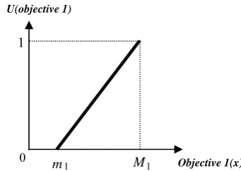
Step 2.3.Calculate the utility of objective function
of Problem 1 as follow:
1 1 1
)
(
1
)
1
(
objective
U
According to Figure 1, when objective1(x)is equal
to extreme values m1 and M1, objective function
acquires minimum and maximum utility, respectively. Otherwise, it varies between 0 and 1 per unit change in objective 1(x).
Figure 1. The utility function of Problem 1
0 m
1
M Objective 1(x)
M
m
U(objective 1)
objective x
m
U objective objective x m M m
( 2) 1 2( ) 2
2 2
Problem 2 as follow:
Calculate the utility of objective function of 2
M. Step 3.3.
the resulted optimized objective value
maximization and solve the new Problem 2. Name Convert the objective function of Problem 2 to 2
m . Step 3.2.
name the optimized objective value
Problem 2 by one of the optimization softwares and Step 3.1. Solve and follow the subsequent steps:
Step 3.Call the minimization problem as Problem 2
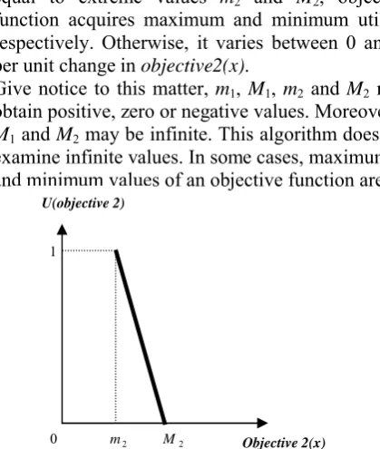
According to Figure 2, when objective2(x) is
equal to extreme values m2 and M2, objective
function acquires maximum and minimum utility, respectively. Otherwise, it varies between 0 and 1 per unit change in objective2(x).
Give notice to this matter, m1, M1, m2 and M2 may
obtain positive, zero or negative values. Moreover,
M1and M2may be infinite. This algorithm does not
examine infinite values. In some cases, maximum and minimum values of an objective function are
Figure 2. The utility function of Problem 2
the same. Given this situation, the utility function of considered objective function is converted to a single-point which is always equivalent to 1.
Step 4. Initially, set t10and t2 0.
Step 5. Calculate the proper reduction amount in utility of each objective functions as follow:
1 1
1 1
11
Min Max
Obj t
Ut
2 2
2 2
22 Max Min
Obj t
U t
where Obj1 and Obj2 are assumed to be unit
change amount in objective1(x) and objective2(x),
respectively. Then, compute the reduced utility values as below:
1
1 1
1 ) 1
(Objt Ut U
2
2 2
2 ) 1
(Objt U t
U
Change t2 from 0 to
2 2 2
Obj Min Max
in above
formulas. In each iteration, note the value of
) (Obj1t1
U ,U(Obj2t2),Obj1t1,Obj2t2 and add the
equations objective 1(x)= Obj1t1and objective2(x)= 2
2t
Obj to the constraints of main problem. Solve the obtained problem that has no objective function.
Two cases may occur: a) there is a feasible solution in this iteration and take notice of it, b) there is no feasible solution. Step 6. t1t11. If
1 1 1 1
Obj Min Max t
, go to Step 5; else, all possible
situations have been checked and stop.
Step 7. Among the achieved feasible solutions, select the answer that has the highest utility. This choice depends on DM’s point of view about objective functions.
4. COMPUTATIONAL RESULTS
In order to examine the performance of proposed solution procedure, a numerical example is presented in this section. Some characteristics of the example are summarized in Table 1. The number of employees is considered 24 persons. In this instance, each employee has just one specialization and employees of each specialization are classified into three skill levels (Senior, Standard and Junior). The planning period is 28 days (4 weeks). Table 2 shows the specialization and real skill level of each employee.
Apart from the junior skill level of the first specialization in a morning shift of all days, the number of required employees at any skill level of each specialization is one person in all shifts of planning horizon’s days. The required number of junior employees of the first specialization in a morning shift of all days is two persons. According to problem’s assumptions, each employee can be assigned to work at his/her real skill level or at any lower skill levels in his/her specialization but not more than one skill level simultaneously. Hence, senior employees are capable to work at standard or junior level and standard employees have ability to work at junior level of his/her specialization.
Some employees are interested in working at a special skill level in some shifts/all shifts of some days. Table 3 demonstrates the shifts that these employees have requested to be assigned at their desired skill levels.
Regarding above information, the presented bi-objective manpower scheduling problem is solved by the Lingo 9 software in accordance with the steps of proposed algorithm and the results are expressed in Tables 4 and 5.
In this case, the DM is interested in obtaining the feasible solution in which both objective functions 1
U(objective 2)
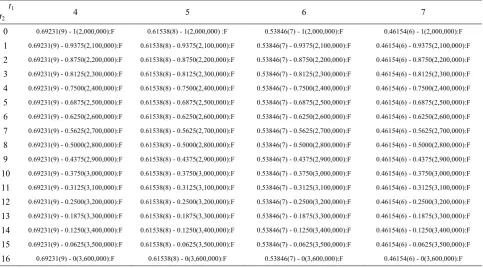
have the highest utility at the same time. Therefore, it is not mandatory to check all situations and as soon as to reach the highest utility simultaneously, the algorithm can be stopped. Table 5 summarizes all examined situations. 1(13)-0.9375(2,100,000):N at t1=0 and t2=1 indicates that the first objective
function has the utility value of 1 at the objective value of 13, the second objective function has the utility value of 0.9375 at the objective value of 2,100,000, and a non-feasible solution in this iteration. For instance, the DM chooses a feasible solution including U(Obj1)= 0.92308 at Obj1=12
and U(Obj2)= 0.9375 at Obj2=2,100,000. Table 6
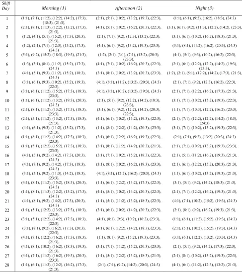
shows the shift-assignment of employees in a selected solution by the DM. In some shifts, employees have been allotted to lower skill levels than their real skill. For example, (1:3) in the sixth day and the morning shift implies that an employee with ID=1 has been assigned to work in the morning shift of the sixth day of planning period at a junior skill level of his/her specialization.
The selected feasible solution is an effective (a dominant) point for the proposed bi-objective manpower scheduling problem. Getting far from this point causes the situation of one of objective functions to get worse.
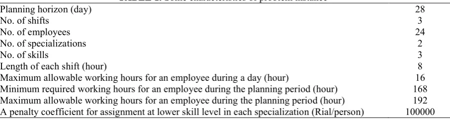
TABLE 1. Some characteristics of problem instance
Planning horizon (day) 28
No. of shifts 3
No. of employees 24
No. of specializations 2
No. of skills 3
Length of each shift (hour) 8
Maximum allowable working hours for an employee during a day (hour) 16 Minimum required working hours for an employee during the planning period (hour) 168 Maximum allowable working hours for an employee during the planning period (hour) 192 A penalty coefficient for assignment at lower skill level in each specialization (Rial/person) 100000
TABLE 4. The values obtained by the proposed algorithm
m1 0 (person) m2 2,000,000 (Rial)
M1 13 (person) M2 3,600,000 (Rial) 1
Obj
1(person) Obj2 100,000 (Rial)
1 1 Min
Max 13 (person) Max2Min2 1,600,000 (Rial)
1
t 0,1,…,13 t2 0,1,…,16
TABLE 2. The specialization and real skill level of each employee
Employee’s ID Specialization Real skill level
1,2,3,4 1 Senior (1)
5,6,7,8 2 Senior (1)
9,10,11,12 1 Standard (2)
13,14,15,16 2 Standard (2)
17,18,19,20 1 Junior (3)
21,22,23,24 2 Junior (3)
TABLE 3. The List of employees that have tendency to work at a special skill level in some shifts/days
Employee’s ID Skill Day Shift
1 1-2-3 1 Morning (1)- Afternoon (2)- Night (3)
1 2-3 2 Morning (1)- Afternoon (2)- Night (3)
1 2-3 3 Morning (1)- Afternoon (2)- Night (3)
1 2-3 4 Morning (1)- Afternoon (2)- Night (3)
1 2-3 5 Morning (1)- Afternoon (2)- Night (3)
1 2-3 6 Morning (1)- Afternoon (2)- Night (3)
1 2-3 7 Morning (1)- Afternoon (2)- Night (3)
1 1 10 Morning (1)
10 2-3 17 Morning (1)- Afternoon (2)- Night (3)
13 2 22 Morning (1)
16 2 16 Night (3)
19 3 1 Afternoon (2)
Cont’d TABLE 5. Utility and objective values in all iterations (U1(Obj1t1) -U2(Obj2t2):feasible/non-feasible)
t1
t2 4 5 6 7
0 0.69231(9) - 1(2,000,000):F 0.61538(8) - 1(2,000,000) :F 0.53846(7) - 1(2,000,000):F 0.46154(6) - 1(2,000,000):F
1 0.69231(9) - 0.9375(2,100,000):F 0.61538(8) - 0.9375(2,100,000):F 0.53846(7) - 0.9375(2,100,000):F 0.46154(6) - 0.9375(2,100,000):F
2 0.69231(9) - 0.8750(2,200,000):F 0.61538(8) - 0.8750(2,200,000):F 0.53846(7) - 0.8750(2,200,000):F 0.46154(6) - 0.8750(2,200,000):F
3 0.69231(9) - 0.8125(2,300,000):F 0.61538(8) - 0.8125(2,300,000):F 0.53846(7) - 0.8125(2,300,000):F 0.46154(6) - 0.8125(2,300,000):F
4 0.69231(9) - 0.7500(2,400,000):F 0.61538(8) - 0.7500(2,400,000):F 0.53846(7) - 0.7500(2,400,000):F 0.46154(6) - 0.7500(2,400,000):F
5 0.69231(9) - 0.6875(2,500,000):F 0.61538(8) - 0.6875(2,500,000):F 0.53846(7) - 0.6875(2,500,000):F 0.46154(6) - 0.6875(2,500,000):F
6 0.69231(9) - 0.6250(2,600,000):F 0.61538(8) - 0.6250(2,600,000):F 0.53846(7) - 0.6250(2,600,000):F 0.46154(6) - 0.6250(2,600,000):F
7 0.69231(9) - 0.5625(2,700,000):F 0.61538(8) - 0.5625(2,700,000):F 0.53846(7) - 0.5625(2,700,000):F 0.46154(6) - 0.5625(2,700,000):F
8 0.69231(9) - 0.5000(2,800,000):F 0.61538(8) - 0.5000(2,800,000):F 0.53846(7) - 0.5000(2,800,000):F 0.46154(6) - 0.5000(2,800,000):F
9 0.69231(9) - 0.4375(2,900,000):F 0.61538(8) - 0.4375(2,900,000):F 0.53846(7) - 0.4375(2,900,000):F 0.46154(6) - 0.4375(2,900,000):F
10 0.69231(9) - 0.3750(3,000,000):F 0.61538(8) - 0.3750(3,000,000):F 0.53846(7) - 0.3750(3,000,000):F 0.46154(6) - 0.3750(3,000,000):F
11 0.69231(9) - 0.3125(3,100,000):F 0.61538(8) - 0.3125(3,100,000):F 0.53846(7) - 0.3125(3,100,000):F 0.46154(6) - 0.3125(3,100,000):F
12 0.69231(9) - 0.2500(3,200,000):F 0.61538(8) - 0.2500(3,200,000):F 0.53846(7) - 0.2500(3,200,000):F 0.46154(6) - 0.2500(3,200,000):F
13 0.69231(9) - 0.1875(3,300,000):F 0.61538(8) - 0.1875(3,300,000):F 0.53846(7) - 0.1875(3,300,000):F 0.46154(6) - 0.1875(3,300,000):F
14 0.69231(9) - 0.1250(3,400,000):F 0.61538(8) - 0.1250(3,400,000):F 0.53846(7) - 0.1250(3,400,000):F 0.46154(6) - 0.1250(3,400,000):F
15 0.69231(9) - 0.0625(3,500,000):F 0.61538(8) - 0.0625(3,500,000):F 0.53846(7) - 0.0625(3,500,000):F 0.46154(6) - 0.0625(3,500,000):F
16 0.69231(9) - 0(3,600,000):F 0.61538(8) - 0(3,600,000):F 0.53846(7) - 0(3,600,000):F 0.46154(6) - 0(3,600,000):F
TABLE 5. Utility and objective values in all iterations (U1(Obj1t1) -U2(Obj2t2):feasible/non-feasible)
t1
t2 0 1 2 3
0 1(13) - 1(2,000,000):N 0.92308(12) - 1(2,000,000):N 0.84615(11) - 1(2,000,000):F 0.76923(10) - 1(2,000,000):F
1 1(13) - 0.9375(2,100,000):N 0.92308(12) - 0.9375(2,100,000):F 0.84615(11) - 0.9375(2,100,000):F 0.76923(10) - 0.9375(2,100,000):F
2 1(13) - 0.8750(2,200,000):F 0.92308(12) - 0.8750(2,200,000):F 0.84615(11) - 0.8750(2,200,000):F 0.76923(10) - 0.8750(2,200,000):F
3 1(13) - 0.8125(2,300,000):F 0.92308(12) - 0.8125(2,300,000):F 0.84615(11) - 0.8125(2,300,000):F 0.76923(10) - 0.8125(2,300,000):F
4 1(13) - 0.7500(2,400,000):F 0.92308(12) - 0.7500(2,400,000):F 0.84615(11) - 0.7500(2,400,000):F 0.76923(10) - 0.7500(2,400,000):F
5 1(13) - 0.6875(2,500,000) :F 0.92308(12) - 0.6875(2,500,000):F 0.84615(11) - 0.6875(2,500,000):F 0.76923(10) - 0.6875(2,500,000):F
6 1(13) - 0.6250(2,600,000):F 0.92308(12) - 0.6250(2,600,000):F 0.84615(11) - 0.6250(2,600,000):F 0.76923(10) - 0.6250(2,600,000):F
7 1(13) - 0.5625(2,700,000):F 0.92308(12) - 0.5625(2,700,000):F 0.84615(11) - 0.5625(2,700,000):F 0.76923(10) - 0.5625(2,700,000):F
8 1(13) - 0.5000(2,800,000):F 0.92308(12) - 0.5000(2,800,000):F 0.84615(11) - 0.5000(2,800,000):F 0.76923(10) - 0.5000(2,800,000):F
9 1(13) - 0.4375(2,900,000):F 0.92308(12) - 0.4375(2,900,000):F 0.84615(11) - 0.4375(2,900,000):F 0.76923(10) - 0.4375(2,900,000):F
10 1(13) - 0.3750(3,000,000):F 0.92308(12) - 0.3750(3,000,000):F 0.84615(11) - 0.3750(3,000,000):F 0.76923(10) - 0.3750(3,000,000):F
11 1(13) - 0.3125(3,100,000):F 0.92308(12) - 0.3125(3,100,000):F 0.84615(11) - 0.3125(3,100,000):F 0.76923(10) - 0.3125(3,100,000):F
12 1(13) - 0.2500(3,200,000):F 0.92308(12) - 0.2500(3,200,000):F 0.84615(11) - 0.2500(3,200,000):F 0.76923(10) - 0.2500(3,200,000):F
13 1(13) - 0.1875(3,300,000):F 0.92308(12) - 0.1875(3,300,000):F 0.84615(11) - 0.1875(3,300,000):F 0.76923(10) - 0.1875(3,300,000):F
14 1(13) - 0.1250(3,400,000):F 0.92308(12) - 0.1250(3,400,000):F 0.84615(11) - 0.1250(3,400,000):F 0.76923(10) - 0.1250(3,400,000):F
15 1(13) - 0.0625(3,500,000):F 0.92308(12) - 0.0625(3,500,000):F 0.84615(11) - 0.0625(3,500,000):F 0.76923(10) - 0.0625(3,500,000):F
Cont’d TABLE 5. Utility and objective values in all iterations (U1(Obj1t1) -U2(Obj2t2):feasible/non-feasible) t1
t2 8 9 10 11
0 0.38462(5) - 1(2,000,000):F 0.30769(4) - 1(2,000,000):F 0.23077(3) - 1(2,000,000):F 0.15385(2) - 1(2,000,000):F
1 0.38462(5) - 0.9375(2,100,000):F 0.30769(4) - 0.9375(2,100,000):F 0.23077(3) - 0.9375(2,100,000):F 0.15385(2) - 0.9375(2,100,000):F
2 0.38462(5) - 0.8750(2,200,000):F 0.30769(4) - 0.8750(2,200,000):F 0.23077(3) - 0.8750(2,200,000):F 0.15385(2) - 0.8750(2,200,000):F
3 0.38462(5) - 0.8125(2,300,000):F 0.30769(4) - 0.8125(2,300,000):F 0.23077(3) - 0.8125(2,300,000):F 0.15385(2) - 0.8125(2,300,000):F
4 0.38462(5) - 0.7500(2,400,000):F 0.30769(4) - 0.7500(2,400,000):F 0.23077(3) - 0.7500(2,400,000):F 0.15385(2) - 0.7500(2,400,000):F
5 0.38462(5) - 0.6875(2,500,000):F 0.30769(4) - 0.6875(2,500,000):F 0.23077(3) - 0.6875(2,500,000):F 0.15385(2) - 0.6875(2,500,000):F
6 0.38462(5) - 0.6250(2,600,000):F 0.30769(4) - 0.6250(2,600,000):F 0.23077(3) - 0.6250(2,600,000):F 0.15385(2) - 0.6250(2,600,000):F
7 0.38462(5) - 0.5625(2,700,000):F 0.30769(4) - 0.5625(2,700,000):F 0.23077(3) - 0.5625(2,700,000):F 0.15385(2) - 0.5625(2,700,000):F
8 0.38462(5) - 0.5000(2,800,000):F 0.30769(4) - 0.5000(2,800,000):F 0.23077(3) - 0.5000(2,800,000):F 0.15385(2) - 0.5000(2,800,000):F
9 0.38462(5) - 0.4375(2,900,000):F 0.30769(4) - 0.4375(2,900,000):F 0.23077(3) - 0.4375(2,900,000):F 0.15385(2) - 0.4375(2,900,000):F
10 0.38462(5) - 0.3750(3,000,000):F 0.30769(4) - 0.3750(3,000,000):F 0.23077(3) - 0.3750(3,000,000):F 0.15385(2) - 0.3750(3,000,000):F
11 0.38462(5) - 0.3125(3,100,000):F 0.30769(4) - 0.3125(3,100,000):F 0.23077(3) - 0.3125(3,100,000):F 0.15385(2) - 0.3125(3,100,000):F
12 0.38462(5) - 0.2500(3,200,000):F 0.30769(4) - 0.2500(3,200,000):F 0.23077(3) - 0.2500(3,200,000):F 0.15385(2) - 0.2500(3,200,000:F
13 0.38462(5) - 0.1875(3,300,000):F 0.30769(4) - 0.1875(3,300,000):F 0.23077(3) - 0.1875(3,300,000):F 0.15385(2) - 0.1875(3,300,000):F
14 0.38462(5) - 0.1250(3,400,000):F 0.30769(4) - 0.1250(3,400,000):F 0.23077(3) - 0.1250(3,400,000):F 0.15385(2) - 0.1250(3,400,000):F
15 0.38462(5) - 0.0625(3,500,000):F 0.30769(4) - 0.0625(3,500,000):F 0.23077(3) - 0.0625(3,500,000):F 0.15385(2) - 0.0625(3,500,000):F
16 0.38462(5) - 0(3,600,000):F 0.30769(4) - 0(3,600,000):F 0.23077(3) - 0(3,600,000):F 0.15385(2) - 0(3,600,000):F
Cont’d TABLE 5. Utility and objective values in all iterations (U1(Obj1t1) -U2(Obj2t2):feasible/non-feasible)
t1
t2 12 13
0 0.07692(1) - 1(2,000,000):F 0(0) - 1(2,000,000):F
1 0.07692(1) - 0.9375(2,100,000):F 0(0) - 0.9375(2,100,000):F
2 0.07692(1) - 0.8750(2,200,000):F 0(0) - 0.8750(2,200,000):F
3 0.07692(1) - 0.8125(2,300,000):F 0(0) - 0.8125(2,300,000):F
4 0.07692(1) - 0.7500(2,400,000):F 0(0) - 0.7500(2,400,000):F
5 0.07692(1) - 0.6875(2,500,000):F 0(0) - 0.6875(2,500,000):F
6 0.07692(1) - 0.6250(2,600,000):F 0(0) - 0.6250(2,600,000):F
7 0.07692(1) - 0.5625(2,700,000):F 0(0) - 0.5625(2,700,000):F
8 0.07692(1) - 0.5000(2,800,000):F 0(0) - 0.5000(2,800,000):F
9 0.07692(1) - 0.4375(2,900,000):F 0(0) - 0.4375(2,900,000):F
10 0.07692(1) - 0.3750(3,000,000):F 0(0) - 0.3750(3,000,000):F
11 0.07692(1) - 0.3125(3,100,000):F 0(0) - 0.3125(3,100,000):F
12 0.07692(1) - 0.2500(3,200,000):F 0(0) - 0.2500(3,200,000):F
13 0.07692(1) - 0.1875(3,300,000):F 0(0) - 0.1875(3,300,000):F
14 0.07692(1) - 0.1250(3,400,000):F 0(0) - 0.1250(3,400,000):F
15 0.07692(1) - 0.0625(3,500,000):F 0(0) - 0.0625(3,500,000):F
TABLE 6. A shift schedule selected by DM at U(Obj1=12)=0.92308 and U(Obj2=2,100,000)=0.9375 (ID:Skill)
Shift
Day Morning (1) Afternoon (2) Night (3)
1 (1:1), (7:1), (11:2), (12:2), (14:2), (17:3), (18:3), (21:3),
(2:1), (5:1), (10:2), (13:2), (19:3), (22:3), (1:1), (6:1), (9:2), (16:2), (18:3), (24:3)
2 (2:1), (8:1), (11:3), (12:2), (13:2), (17:3), (21:3),
(4:1), (5:1), (10:2), (16:2), (20:3), (22:3), (3:1), (6:1), (9:2), (11:3), (12:2), (14:2), (23:3),
3 (1:2), (4:1), (5:1), (15:2), (17:3), (20:3),
(21:3), (2:1), (7:1), (9:2), (12:3), (13:2), (22:3), (3:1), (6:1), (10:2), (16:2), (18:3), (21:3), 4 (1:2), (2:1), (7:1), (12:3), (15:2), (17:3),
(24:3)
(4:1), (6:1), (9:2), (13:2), (19:3), (23:3), (3:1), (8:1), (11:2), (16:2), (20:3), (24:3)
5 (5:1), (9:2), (15:2), (18:3), (19:3), (21:3), (1:2), (2:1), (3:1), (7:1), (13:2), (20:3),
(23:3), (4:1), (5:1), (9:3), (10:2), (16:2), (22:3),
6 (1:3), (3:1), (8:1), (11:2), (15:2), (17:3), (24:3)
(4:1), (7:1), (10:2), (16:2), (20:3), (22:3), (2:1), (6:1), (12:2), (12:2), (14:2), (19:3), (23:3),
7 (4:1), (5:1), (9:3), (11:2), (15:2), (18:3), (24:3)
(3:1), (8:1), (10:2), (13:2), (20:3), (23:3), (1:2), (2:1), (5:1), (12:2), (14:2), (17:3), (21:3),
8 (3:1), (6:1), (9:3), (10:2), (15:2), (19:3),
(22:3), (4:1), (8:1), (11:2), (13:2), (20:3), (24:3) (2:1), (7:1), (9:2), (12:3), (16:2), (22:3), 9 (3:1), (6:1), (11:2), (15:2), (17:3), (18:3),
(23:3),
(4:1), (8:1), (10:2), (13:2), (19:3), (24:3) (2:1), (7:1), (12:2), (16:2), (17:3), (21:3),
10 (1:1), (6:1), (11:2), (13:2), (19:3), (20:3), (24:3)
(2:1), (5:1), (9:2), (12:2), (14:2), (18:3), (23:3),
(3:1), (7:1), (10:2), (15:2), (19:3), (22:3),
11 (2:1), (8:1), (11:2), (13:2), (17:3), (18:3), (23:3),
(3:1), (6:1), (9:2), (12:2), (14:2), (20:3), (22:3),
(1:1), (7:1), (10:3), (12:2), (16:2), (23:3),
12 (2:1), (5:1), (11:2), (13:2), (17:3), (18:3), (21:3),
(4:1), (6:1), (10:2), (15:2), (19:3), (22:3), (2:1), (7:1), (12:2), (12:2), (14:2), (18:3), (24:3)
13 (4:1), (6:1), (9:3), (11:2), (15:2), (17:3), (21:3),
(1:1), (8:1), (12:2), (14:2), (20:3), (23:3), (3:1), (7:1), (10:2), (15:2), (19:3), (22:3),
14 (1:1), (8:1), (11:2), (14:2), (17:3), (18:3), (23:3),
(3:1), (6:1), (12:2), (16:2), (19:3), (22:3), (2:1), (7:1), (9:2), (13:2), (20:3), (24:3)
15 (1:1), (5:1), (12:2), (15:2), (17:3), (18:3), (23:3),
(3:1), (8:1), (11:2), (14:2), (20:3), (21:3), (2:1), (7:1), (10:2), (13:2), (19:3), (23:3),
16 (4:1), (5:1), (9:2), (14:2), (17:3), (20:3), (24:3)
(3:1), (7:1), (10:2), (15:2), (18:3), (22:3), (2:1), (5:1), (11:2), (16:2), (19:3), (21:3),
17 (4:1), (7:1), (9:2), (14:2), (17:3), (18:3), (24:3)
(3:1), (8:1), (10:2), (16:2), (19:3), (23:3), (2:1), (6:1), (12:2), (15:2), (20:3), (21:3),
18 (3:1), (5:1), (9:2), (11:3), (14:2), (18:3),
(23:3), (4:1), (8:1), (12:2), (16:2), (20:3), (24:3) (1:1), (6:1), (10:2), (13:2), (19:3), (21:3), 19 (4:1), (8:1), (11:2), (15:2), (18:3), (20:3),
(24:3)
(1:1), (6:1), (12:2), (13:2), (17:3), (22:3), (3:1), (5:1), (9:2), (14:2), (18:3), (21:3),
20 (1:1), (8:1), (11:3), (12:2), (13:2), (17:3),
(24:3) (4:1), (5:1), (10:2), (14:2), (20:3), (22:3), (2:1), (7:1), (12:2), (16:2), (19:3), (21:3), 21 (4:1), (8:1), (9:2), (14:2), (17:3), (20:3),
(24:3)
(1:1), (5:1), (11:2), (13:2), (18:3), (22:3), (4:1), (7:1), (10:2), (15:2), (19:3), (24:3)
22 (1:1), (5:1), (12:2), (13:2), (17:3), (18:3), (23:3),
(3:1), (6:1), (10:2), (14:2), (20:3), (22:3), (2:1), (8:1), (9:2), (16:2), (19:3), (21:3),
23 (3:1), (5:1), (12:2), (14:2), (17:3), (18:3), (22:3),
(4:1), (8:1), (9:3), (10:2), (16:2), (23:3), (1:1), (6:1), (11:2), (15:2), (19:3), (24:3)
24 (3:1), (8:1), (9:2), (16:2), (17:3), (20:3), (22:3),
(4:1), (6:1), (12:2), (14:2), (18:3), (23:3), (2:1), (5:1), (10:2), (15:2), (19:3), (24:3)
25 (4:1), (7:1), (12:2), (16:2), (17:3), (18:3), (21:3),
(1:1), (8:1), (9:2), (15:2), (19:3), (23:3), (3:1), (6:1), (12:2), (13:2), (20:3), (24:3)
26 (4:1), (8:1), (10:2), (16:2), (18:3), (19:3), (21:3),
(3:1), (7:1), (11:2), (15:2), (20:3), (23:3), (2:1), (5:1), (9:2), (14:2), (17:3), (22:3),
27 (4:1), (7:1), (11:2), (16:2), (19:3), (20:3), (23:3),
(1:1), (5:1), (12:2), (13:2), (18:3), (21:3), (2:1), (8:1), (10:2), (15:2), (19:3), (22:3),
28 (1:1), (6:1), (11:3), (12:2), (16:2), (17:3), (21:3),
5. CONCLUDING REMARKS
In this paper, a novel bi-objective manpower scheduling problem that is appropriate for production and service environments was introduced. The considered objectives has minimized the penalty incurred by the employees’ assignment at lower skill levels than their real skill and maximized the employees’ utility by assigning them at desired skill levels in some shifts/days. Also, a solution procedure on the basis of utility of objective values was proposed. Solving the given problem by proposed procedure, a feasible solution that is an effective point for presented bi-objective model was obtained. Getting far from the acquired effective point makes the situation of one of objective functions to get worse.
In this study, the utilty of objective values was considered as a linear function. Since the utility function can have various forms, it can be taken as a non-linear function into account according to DM’s desire.
6. REFERENCES
1. Castillo I., Joro T., Li Y.Y., “Workforce scheduling with multiple objectives”, European Journal of Operational Research,Vol. 196, (2009), 162-170.
2. Beaulieu H., Ferland J.A., Gendron B., Michelon P., “A mathematical programming approach for scheduling physicians in the emergency room”, Health Care Management Science, Vol. 3, (2000), 193-200.
3. Valls V., Perez A., Quintanilla S., “Skilled workforce scheduling in service centers”, European Journal of Operational Research, Vol. 193, (2009), 791-804. 4. Burns R.N., Carter M.W., “Work force size and single
shift schedules with variable demands”, Management Science, Vol. 31, NO. 5, (1985), 599–607.
5. Burns R.N., Namimhan R., Smith L.D., “An algorithm for scheduling a single category workforce on four-day work weeks”, Working Paper95-11, Queen’s School of Business, 1995.
6. Hung R., “Single-shift workforce scheduling under a compressed workweek”, OMEGA, Vol. 19, NO. 5, (1991), 494–497.
7. Hung R., “An annotated bibliography of compressed workweeks”, International Journal of Manpower, Vol. 17, NO. 6/7, (1996), 43–53.
8. Burns R.N., Koop G.J., “A modular approach to optimal multiple-shift manpower scheduling”, Operations Research, Vol. 35, NO. 1, (1987), 100–110.
9. Burns R.N., Namimhan R., “10-hours multiple shift scheduling”, Working Paper 94-36, Queen’s School of Business, 1994.
10. Hung R., “A three-day workweek multiple-shift
scheduling model”, Journal of the Operational Research Society, Vol. 44, NO. 2, (1993), 141–146.
11. Hung R., “A multiple-shift workforce scheduling model under the 4-day workweek with weekday and weekend labour demands”, Journal of the Operational Research Society, Vol. 45, NO. 9, (1994), 1088–1092.
12. Hung R., “Shiftwork scheduling with phase-delay feature”, International Journal of Production Research, Vol. 35, NO. 7, (1997), 1961–1968.
13. Hung R., “Scheduling for continuous operations: The Baylor plan”, International Journal of Materials and Product Management, Vol. 12, NO. 1, (1997), 37–42. 14. Azmat C.S., Widmer M., “A case study of single shift
planning and scheduling under annualized hours: A simple three-step approach”, European Journal of Operational Research, Vol. 153, NO. 1, (2004), 48-175. 15. Tiberwala R.D., Philippe D., Browne J., “Optimal
Scheduling of two consecutive idle periods”, Management Science, Vol. 19, NO. 1, (1972). 71-75. 16. Baker K.R., “Scheduling a full-time workforce to meet
cyclic staffing requirements”, Management Science, Vol. 20, NO. 12, (1974), 1561-1568.
17. Baker K.R., Magazine M.-T., “Workforce scheduling with cyclic demands and days-off constraints”, Management Science, Vol. 24, (1977), 161-167.
18. Hung R., “Multiple shift workforce scheduling under the 3-4 workweek with different weekday and weekend labor requirements”, Management Science, Vol. 40, NO. 2, (1994), 49-57.
19. Alfares H.K., “Four day workweek scheduling with two or three consecutive days off”, Journal of Mathematical Modeling and Algorithms, Vol. 2, NO. 1, (2003), 67-80. 20. Hung R., “Single shift off-day scheduling of a
hierarchical workforce with variable demands”, European Journal of Operational Research, Vol. 78, NO. 1, (1994), 280-284.
21. Emmons H., Fuh D., “Sizing and Scheduling a full-time and part-time workforce with off-day and off weekend constraints”, Annals of Operations Research, Vol. 70, (1997), 473-492.
22. Narasimhan R., “An Algorithm for multiple shift scheduling of hierarchical workforce on four-day or three-day workweeks”, Information Systems and Operational Research, Vol. 38, NO. 1, (2000), 14-32. 23. Azmat C.S., Hurlimann T., Widmer M., “Mixed integer
programming to schedule a single-shift workforce under annualized hours”, Annals of Operations Research, Vol. 128, (2004), 199-215.
24. Costa M.C., Jarray F., Picouleau C., “An acyclic days-off scheduling problem”, 4OR: A Quarterly Journal of Operations Research, Vol. 4, (2006), 73-85.
25. Cerulli R., Gaudioso M., Mautone R., “A class of manpower scheduling problems”, Methods and Model of Operations Research, Vol. 105, (1992), 36- 93.
26. Emmons H., Fuh D.S., “Sizing and scheduling a full-time and part-time workforce with off-day and off-weekend constraints”, Annals of Operations Research, Vol. 70, (1997), 473-492.
27. Blochliger I., “Modeling staff scheduling problems: A tutorial”, European Journal of Operational Research, Vol. 158, NO. 3, (2004), 533–543.
cyclic days-off scheduling”, Computers Operations Research, Vol. 25, NO. 11, (1998), 9193-923.
29. Lagodimos A.G., Leopoulos V., “Greedy heuristic algorithms for manpower shift planning”, International Journal of Production Economics, Vol. 68, (2000), 95-106.
30. Musliu, N., Gartner, J., Slany, W., “Efficient generation of rotating workforce schedules”, Discrete Applied Mathematics, Vol. 118, NO. 1-2, (2002), 85–98.
31. Ernst A.T., Jiang E., Krishnamoorthy M., Sier D., “Staff scheduling and rostering: A review of applications, methods and models”, European Journal of Operational Research, Vol. 153, (2004), 3-27.
32. Ingolfsson, A., Haque Md, A., Umnikov, A., “Accounting for time-varying queueing effects in workforce scheduling”, European Journal of Operational Research, Vol. 139, NO. 3, (2002), 585–597.
33. Glover F., McMillan C., “The general employee scheduling problem: An integration of management science and artificial intelligence”, Computers and Operations Research, Vol. 13, (1986), 563–593.
34. Willis R., Huxford S., “Staffing rosters with breaks: A case study”, Journal of the Operational Research Society, Vol. 42, (1991), 727–731.
35. Schindler S., Semmel T., “Station staffing at Pan American World Airways”, Interfaces23 (1993) 91–98. 36. Dowsland K., “Nurse scheduling with tabu search and
strategic oscillation”, European Journal of Operational Research, Vol. 106, (1998), 393–407.
37. Bard J.F., Binici C., deSilva A.H., “Staff scheduling at the United States postal service”, Computers and Operations Research, Vol. 30, (2003), 745–771.
38. Eitzen G., Panton D., Mills G., “Multi-skilled workforce optimization”, Annals of Operations Research, Vol. 127, (2004), 359-372.
39. Billonnet A., “Integer programming to schedule a
hierarchical workforce with variable demand”,European Journal of Operational Research, Vol. 114, (1999), 105-114.
40. Cai X., Li K.N., “A genetic algorithm for scheduling staff of mixed skills under multi-criteria”, European Journal of Operational Research, Vol. 125, (2000), 359-369. 41. Techawiboonwong A., yenradee P., Das S.K., “A master
scheduling model with skilled and unskilled temporary workers”, International Journal of Production Economics, Vol. 103, (2006), 798-809.
42. Mohan S., “Scheduling part-time personnel with availability restrictions and preferences to maximize employee satisfaction”, Mathematical and Computer Modeling, Vol. 48, (2008), 1806-1813.
43. Hertz A., Lahrichi N., Widmer M., “A flexible MILP model for multiple-shift workforce planning under annualized hours”, European Journal of Operational Research, Vol. 200, (2010), 850-873.
44. Varadharajan T.K., Rajendran C., “A multi-objective simulated-annealing algorithm for scheduling in flowshops to minimize the makespan and total flowtime of jobs”, European Journal of Operational Research, Vol. 167, (2005), 772-795.
45. Choobineh F.F., Mohebbi E., Khoo H., “A multi-objective tabu search for a single machine scheduling problem with sequence-dependent setup times”, European Journal of Operational Research, Vol. 175, (2006), 318-337.
46. Yagmahan B., Yenisey M.M., “A multi-objective ant colony system algorithm for flowshop scheduling problem”, Expert Systems with Applications, Vol. 37, (2010), 1361-1368.