A NOVEL METHOD FOR DESIGNING AND
OPTIMIZATION OF NETWORKS
A. Sadegheih*
Department of Industrial Engineering, Faculty of Engineering Yazd University, P.O. Box 89195-741, Yazd, Iran
*Corresponding Author
(Received: July 31, 2006 - Accepted in Revised Form: January 18, 2007)
Abstract In this paper, system planning network is formulated with mixed-integer programming. Two meta-heuristic procedures are considered for this problem. The cost function of this problem consists of the capital investment cost in discrete form, the cost of transmission losses and the power generation costs. The DC load flow equations for the network are embedded in the constraints of the mathematical model to avoid sub-optimal solutions that can arise if the enforcement of such constraints is done in an indirect way. The solution of the model gives the best line additions, and also provides information regarding the optimal generation at each generation point. This method of solution is demonstrated on the expansion of a 5 bus-bar system to 6 bus-bars.
Keywords System Planning, Simulated Annealing, Genetic Algorithm, Mathematical Programming, Artificial Intelligence, Iterative Improvement Methods, Heuristic Techniques
ﻩﺪﻴﻜﭼ
ﻭ ﻲﺠﻳﺭﺪﺗﻩﺪﻨﻨﻛ ﺩﺮﺳ ،ﻂﻠﺘﺨﻣ ﺢﻴﺤﺻ ﺩﺍﺪﻋﺍ ﻱﺰﻳﺭ ﻪﻣﺎﻧﺮﺑ ﻪﻠﻴﺳﻮﺑ ﻪﻜﺒﺷ ﻱﺰﻳﺭ ﻪﻣﺎﻧﺮﺑ ﻪﻟﺎﻘﻣﻦﻳﺍ ﺭﺩ
ﺖﺳﺍ ﻩﺪﺷﻱﺯﺎﺳﻝﺪﻣﻚﻴﺘﻧﮊﻢﺘﻳﺭﻮﮕﻟﺍ
.
ﺴﻣ ﻦﻳﺍﻱﺍﺮﺑﻑﺪﻫﻊﺑﺎﺗ
ﺎ
ﻭﺕﺎﻔﻠﺗ،ﻱﺭﺍﺬﮔﻪﻳﺎﻣﺮﺳﻱﺎﻫ ﻪﻨﻳﺰﻫﻞﻣﺎﺷﻪﻟ
ﻲﻣﺎﻫﺭﻮﺗﺍﺮﻧﮊ
ﺪﺷﺎﺑ .
ﺑﻪﻜﺒﺷﻱﺍﺮﺑﺭﺎﺑﻥﺎﻳﺮﺟﺕﻻﺩﺎﻌﻣ
ﻪ
ﺘﻳﺩﻭﺪﺤﻣﻥﺍﻮﻨﻋ
ﺖﺳﺍﻩﺪﺷﻪﺘﻓﺮﮔﺮﻈﻧﺭﺩﺎﻬ
.
ﻞﺣﺖﻳﺎﻬﻧﺭﺩ
ﺴﻣ ﺎ
ﻲﻣﺖﺳﺪﺑﺍﺭﻂﺧﺕﺎﻓﺎﺿﺍﻦﻳﺮﺘﻬﺑﻪﻟ
ﺺﺨﺸﻣﺍﺭﺭﺎﺑﺱﺎﺑﺮﻫﺭﺩﻪﻨﻴﻬﺑﻱﺎﻫﺭﻮﺗﺍﺮﻧﮊﻪﺑﻊﺟﺍﺭﻲﺗﺎﻋﻼﻃﺍﻭﺩﺭﻭﺁ
ﻲﻣ ﺪﻨﻛ .
ﺑﺵﻭﺭﻦﻳﺍ
ﻪ
ﺖﺳﺍﻩﺪﺷﻞﺣﺭﺎﺑﺱﺎﺑﺶﺷﻪﺑﺭﺎﺑﺱﺎﺑﺞﻨﭘﺯﺍﻲﻟﺎﺜﻣﻪﻠﻴﺳﻭ
.
1. INTRODUCTION
System network planning expansion is a complex mathematical optimization problem because it involves, typically, a large number of problem variables. The commonly used methods reported in the literature can be categorized into mathematical programming, heuristic based, artificial intelligence and iterative improvement methods [1-22].
As long ago as 1960, Knight [2] used such a method in which starting from the geographical positions of the substations required to interconnect, a set of equations is obtained and solved by linear programming to obtain a minimum cost power transmission network design. The drawback of this method is that the load flow constraints are not taken into consideration. Garver [3] proposed a method which starts by converting the electrical
network expansion problem into a linear programming problem. The mathematical programming technique used in solving the linear network model minimizes a loss function defined as power times a guide number summed over all network links. The overload path with the largest overload is selected for circuit addition. The drawback of this method is that the model has no user interaction and is fixed by program formulation. Villasana et al [1] and Serna et al [4] also proposed methods used a DC linear power flow model and a transportation model respectively. In both methods, the model is intractable.
phase VAR (Voltage Amper Reactive) allocation is specified. In this method, losses have been excluded. Kaltenbach et al [6] proposed a model which uses a combination of linear and dynamic programming techniques to find the minimum cost capacity addition to accommodate a given change in demand and generation. The drawback of this method is that a very large number of decision variables is required.
Farrag and El-Metwally [7] proposed a method, using mixed-integer programming, in which the objective function contains both capital cost represented in its discrete form and the transmission loss cost in a linear form. Kirchhoff’s first and second laws are included in the constraints, in addition to the line security constraints. In this method, the loss term is linearized and a large number of decision variables are required. Sharifnia and Ashtiani [8] proposed a method for the synthesis of a minimum-cost secure network. In this method, the loss terms are linearized in the constraints and a large number of decision variables are required. Adam et al [9] proposed a method which is based on an interpretation of fixed cost transportation type models and includes both network security (in the transmission network) and cost of loss (in the distribution network). The drawback of this method is that the loss term is in a linearized form and it requires a large number of decision variables due to the use of the mixed-integer linear programming technique as the solution tool.
Lee et al [10] proposed a method which is based on static expansion of networks using the zero-one integer programming technique and Romero and Monticelli [11] proposed a zero-one implicit enumeration method for optimizing investments in transmission expansion planning. These methods require a large number of decision variables and are computationally very expensive. Padiyar et al [12] made a comparison of the computation times required by four different optimization techniques: the transportation model; linear; zero-one and non-linear programming. The use of zero-one and non-linear programming requires high CPU times compared to other methods which makes them ineffective for large scale systems [13] and all of the methods reviewed are fixed by program formulation. Yousef and Hackam [14] proposed a model
capable of dealing with both static and dynamic modes of transmission planning, using non-linear programming. The cost function includes the investment and transmission loss cost. Again, this method requires long computation times and a large number of decision variables [15].
El-Sobki et al [16] proposed a heuristic method which is a systematic procedure to cancel the ineffective lines from the network. The process is directed in a good manner such that the minimum cost network will be obtained containing the most effective routes with the best number of circuits. The DC-load flow model is used. The drawback of this method is that power losses are not taken into account.
Albuyeh and Skiles [17] presented a planning method involving three integral parts. The first is a network model using a fast decoupled load flow relating the changes in active and reactive powers to changes in bus angles and voltages, respectively. In the second part, a selection contingency analysis is employed to determine the maximum overload on each branch and the maximum voltage deviation for each bus. Finally, the line cost, maximum overload and a sensitivity matrix are combined into two formulae to determine the branch to be added and the susceptance of that branch. The procedure is repeated until the contingency analysis shows no overload. In this method losses have been included as a linear term.
Ekwue [18] proposed a method derived on the basis of a DC-load flow approach. The method determines the number of lines of each specification to be added to a network to eliminate system overloads at minimum cost. A static optimization procedure, based on the steepest-descent algorithm, is then used to determine the new admittances to be implemented along these rights of way. In this method, the model is only applicable to already connected systems and not expansion as considered here.
In general, a characteristic of heuristic techniques is that strictly speaking an optimal solution is not sought; instead the goal is a “good” solution. Whilst this may be seen as an advantage from the practical point of view, it is a distinct disadvantage if there are good alternative techniques that target the optimal solution.
(AI) theory and techniques, some AI-based approaches to transmission network planning have been proposed in recent years. These include the use of expert systems [19] and artificial neural network (ANN) based [20] methods. The main advantage of the expert system based method lies in its ability to simulate the experience of planning experts in a formal way. However, knowledge acquisition is always a very difficult task in applying this method. Moreover, maintenance of the large knowledge base is very difficult. Research into the application of the ANN to the planning of transmission networks is in the preliminary stages, and much work remains to be done. The potential advantage of the ANN is its inherent parallel processing nature.
In recent years, there has been a lot of interest in the application of simulated annealing (SA) and tabu search (TS) to solving some difficult or poorly characterized optimization problems of a multi-modal or combinatorial nature. SA is powerful in obtaining good solutions to large scale optimization problems and has been applied to the planning of transmission networks [21]. In this reference, the transmission network planning is first formulated as a mixed integer non-linear programming and then solved using SA. Cooling schedule could be important and neighborhood function is crucial to its effectiveness [21]. TS has emerged as a highly efficient, search paradigm for finding quickly high quality solutions to combinatorial problems [22-25]. It is characterized by gathering knowledge during the search, and subsequently profiting from this knowledge. TS has been applied successfully to many complicated combinatorial optimization problems in many areas including power systems [26-27], The drawback of this method is that its effectiveness depends very much on the strategy for tabu list manipulation. Obviously, how to specify the size of the tabu list in the searching process plays an important role in the search for good solutions. In general, the tabu list size should grow with the size of a given problem.
From the above review, in this paper, the application of a genetic algorithm and SA are proposed to solve the system network planning problem.
GA’s are based in concept natural genetic and evolutionary mechanisms working on populations
of solutions in contrast to other search techniques that work on a single solution. Searching not on the real parameter solution space but on a bit string encoding of it, they mimic natural chromosome genetics by applying genetics-like operators in search of the global optimum. An important aspect of GA’s is that although they do not require any prior knowledge or any space limitations such as smoothness, convexity or uni-modality of the function to be optimized, they exhibit very good performance in the majority of applications [28]. They only require an evaluation function to assign a quality value (fitness value) to every solution produced. Another interesting feature is that they are inherently parallel (solutions are individuals unrelated with each other), therefore their implementation on parallel machines reduces significantly the CPU time required [28].
Compared with other optimization methods, GA’s are suitable for traversing large search spaces since they can do this relatively rapidly and because the use of mutation diverts the method away from local minima, which will tend to become more common as the search space increases in size. GA’s give an excellent trade-off between solution quality and computing time and flexibility for taking into account specific constraints in real situations.
2. FORMULATION OF THE SYSTEM PLANNING MODEL
Minimize:
Gk P NG
k Ck
NE
1
i Si(PEi PEi) NP
1 i
NS(i)
1
j (Cij(Zij Zij) Lij(Pij Pij )) Z
∑ ∈ + ∑
=
− + + ∑
= ∑= +
− + + + − + + =
(1) Subject to:
Gk P Lk P ) Ej P Ej P k e(j) SE(k) j ( k s(j) SE(k)
j (PEj PEj)
) ij P k e(i) SP(k) i NS(i) 1 j (Pij ) ij P ij P k s(i) SP(k) i NS(i) 1 j ( − = − − + ∑ = ∈ + ∑ = ∈ + − − + − ∑ = ∈ ∑= − + + + − − ∑ = ∈ ∑= (2) • The loop equation l = 1, 2, ..., LBE, containing
only existing lines, this constraint upholds Kirchhoff’s Second Law for existing lines:
0 ) Ei P Ei P ( ) ( LE
i XEi
= − − + ∑
∈ l (3)
• The loop equations for loop l containing one proposed line i:
) ) i ( NS 1 k ) i ( NS 1 k ik Z ik Z ( 1 ( K ) k i P k i P ( Pik X ) LP( k ) Ek P Ek P ( Ek X ∑ = ∑= − + + − ≤ − − + ∑ ∈ + − − + l (4) LBP ..., 2, 1, ) (i) NS 1 k NS(i) 1
k (Zik Zik) 1 ( K ) ik P ik P ( Pik X ) LP(
k XEk(PEk PEk)
= ∑ = ∑= − − + + ≥ − − + ∑ ∈ + − − + l l (5) • The exclusivity constraint for each proposed
line i. This constraint forces the program to select one state only for each proposed line, or delete all its states. The exclusivity constraints result from the fact that the capacity of any line can take on only one value. That value, however, may be any of the discrete capacities in the cost-capacity curve. The exclusivity constraints prevent the capacity from assuming more than one value.
1 ) (i) NS 1 j ij Z ij Z ( ≤ ∑ = − +
+ (6)
• The overload constraint for each existing line i:
NE ..., 2, 1, i Mi E Ei P Ei
P+ + − ≤ = (7)
• The overload constraint for the state j of each proposed line i:
) i ( NS ..., 2, 1, = j NP ..., 2, 1, i ) ij Z ij Z ( Mij P ij P ij P ) ij Z ij Z ( ' Mij P = − + + ≤ − + + ≤ − + + (8)
• The generator capacity limit at each bus-bar k:
Mk P Gk
P ≤ (9)
• The availability constraint at each bus-bar k-this controls the number of lines connected to each bus-bar according to parameter MPK:
NB ..., 2, 1, k Pk M ) (k) SP i ) i ( NS 1
j (Zij Zij = ≥ ∑ ∈ ∑= − + + (10) and NG k ), i ( NS NP, j i, NE, i 0 k G P , ij P , ij P , Ei P , Ei P ∈ ∀ ∈ ∀ ∈ ∀ ≥ − + − + (11) ) i ( NS NP, j i, 1 0, ij Z , ij
Z+ −= ∀ ∈ (12)
The objective function Z consists of the capital investment cost in its discrete form, the cost of transmission losses and cost of generation.
3. SYSTEM DESCRIPTION
Using the 6 bus-bar system planning network introduced in reference 1, a single-stage transmission expansion problem is derived.
made in the light of the following factors: • only one line type is assumed; • the maximum number of states = 4; • the cost of a circuit is proportional to the
line length, therefore, the line length can be used to replace the cost in the comparison analysis.
For this system the following additions have been made: four circuits for line (6,2), two circuits for line (6,4) and one circuit for line (3,5).
4. GA APPLIED TO MIXED-INTEGER SYSTEM PLANNING
The work presented here was carried out using the MicrosoftR ExcelTM spreadsheet and an add-in to provide the GA. This add-in is called EvolverTM and is developed and supplied by Axcelis [29]. The model of network planning developed in this research is built in ExcelTM using the spreadsheet's built-in functions. After building the model, the GA is run to optimize the network given an objective function. The fitness value and decision variables are passed back to the GA component which is independent of the spreadsheet model. At the end of the GA run, when the stopping criterion is met, the best network is presented in a tabular form in the spreadsheet.
The chromosome structure used to represent a particular set of possible transmission line power capacities, for the mixed-integer transmission network planning using GA has nine state variables. Each individual line capacity is encoded by sufficient bits to cover its allowable range of values. The initial population is generated randomly, that is, each bit in each chromosome is set randomly to either 1 or 0. Whenever a new chromosome is generated it is checked to see that in decoded form it produces valid values for the genes. When an invalid value is produced the chromosome is discarded and another one is generated.
The spreadsheet model is developed for solving this problem. In the next step for solving the system planning using a GA, Equation 2 as Kirchhoff’s First Law and Equations 7 to 11 must
be satisfied. Equations 3-5 as Kirchhoff’s Second Law are used to penalize solutions in the cost function.
The final step in the implementation of the system planning using a GA is the fitness function. The fitness value of a chromosome is a measure of how well it meets the desired objective [30-32]. In this case the objective is the minimization of the network’s cost function. Choosing and formulating an appropriate objective function is crucial to the efficient solution of any given genetic algorithm problem. When designing an objective function for an optimization problem with constraints, penalty functions can be introduced and applied to individuals that violate the imposed constraints. The fitness function in Equation 1 with penalty functions is used to calculate the fitness value of each individual.
The following additions have occurred in the system planning: four circuits for line (6,2), two circuits for line (6,4) and one circuit for line (3,5). These additions are the same as those obtained with mixed-integer programming.
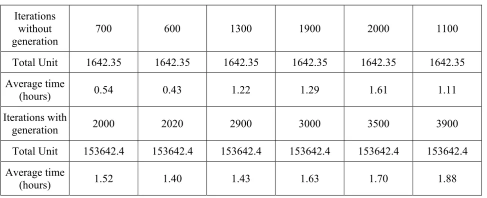
In the GA approach the parameters that influence its performance include population size, crossover rate and mutation rate. A population size of 50, crossover rate 0.5 and mutation rate 0.006 for the system network planning with and without the generation cost are used. Total unit costs are 153642.4 and 1642.35 for the transmission network planning with and without the generation cost respectively. These results are the same as those obtained with mixed-integer programming. Table 1 shows the total unit cost, iterations and the computational time using genetic algorithm.
5. SIMULATED ANNEALING APPLIED TO MIXED - INTEGER SYSTEM
PLANNING
TABLE 1. Total Unit Cost, Iterations and the Computational Time Using GA.
Iterations without generation
700 600 1300 1900 2000 1100
Total Unit 1642.35 1642.35 1642.35 1642.35 1642.35 1642.35
Average time
(hours) 0.54 0.43 1.22 1.29 1.61 1.11
Iterations with
generation 2000 2020 2900 3000 3500 3900
Total Unit 153642.4 153642.4 153642.4 153642.4 153642.4 153642.4 Average time
(hours) 1.52 1.40 1.43 1.63 1.70 1.88
gradual cooling process of solid materials. However this analogy is limited to the physical movement of the molecules without involving complex thermodynamic systems. Physical annealing refers to the process of cooling a solid material so that it reaches a low energy state. Initially the solid is heated up to melting point. Then it is cooled very slowly, allowing it is to come to thermal equilibrium at each temperature. This process of slow cooling is called annealing. The goal is to find the best arrangement of molecules that minimizes the energy of the system, which is referred to as the ground state of the solid material. If the cooling process is fast, the solid will not attain the ground state, but a locally optimal structure. The analogy between physical annealing and simulated annealing can be summarized as follows:
• The physical configurations or states of the molecules correspond to the optimization solution,
• The energy of the molecules corresponds to the objective function or cost function, • A low energy sate corresponds to an
optimal solution,
• The cooling rate corresponds to the control parameter which will affect the acceptance probability.
The algorithm consists of four main components:
• Configurations,
• Re-configuration technique, • Cost function and
• Cooling schedule [33-40].
By using the Boltzmann distribution, the Metropolis algorithm was to accept uphill moves with a probability of:
) j KT
ΔE ( exp ] Accept [
P = − (13)
Where
i E j E
ΔE= −
The simulated annealing algorithm was employed to solve the problems of mixed-integer programming. The same nine state variables representation scheme applied in the case of the GA was implemented for simulate annealing because of its flexibility and ease of computation. The cost function for this problem is the objective function given in Equation 1. The annealing process stared at a high temperature, T = 1000 units, so most of the moves were accepted.
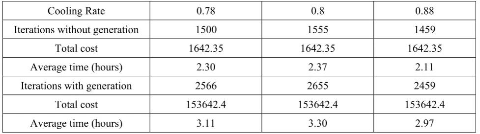
The algorithm was implemented in Turbo C++. The initial stopping criterion was set at a total unit cost of the optimal solution found by the GA. Experiments were conducted again with a lowered stopping criterion. However no improvement was found even after 23.30 and 15 hours computation time for the transmission network planning with and without the generation cost respectively. Ten cooling rates were used (0.50, 0.60, 0.75, 0.78, 0.80, 0.88, 0.93, 0.95, 0.97, 0.99). The final cost function is shown in Table 2 the maximum number of iterations was set at 3000 and 1900 for the transmission network planning with and without the generation cost respectively. Therefore the solution found by the GA was accepted as the optimal solution the final system planning is shown in Tables 2 and 3.
6. CONCLUSIONS
The basic model for system planning network has been described and formulated with mixed-integer programming and two meta-heuristic procedures (GA and SA) were introduced to solve it. The cost function of this problem consists of the capital investment cost in discrete form, the cost of transmission losses and the power generation costs. It is advantageous to use exact DC load flow constraint equations based on the modified form of Kirchhoff’s Second Law because the iterative process for line addition is not required. Hence, the computation time is decreased. To solve system planning for the 6 bus-bar system with the mixed-integer programming requires a large number of variables (zero-one and state variables) resulting in a large number of S, solution space; f, objective function to be
minimised;
N, neighbourhood structure
1. Select a starting solution S0, S0 ∈ S. 2. REPEAT
Randomly select S' as new solution
(S'∈N(S0)); IF f(S') f(S0)
p THEN
S0 =S;' END
UNTIL f(S')ff(S0) for all S'∈N(S0) 3. 0S is the optimal solution.
Figure 1. Local search method.
S, solution space; f, objective function to be minimised;
N, neighbourhood structure
1. Select a starting solution S0, S0 ∈ S; 2. Set an initial temperature, T0 f0; 3. Set a temperature reduction factor
(cooling rate), λ; 4. REPEAT
Randomly select S'∈N(S0); ΔE=f(S')−f(S0);
IF ΔEp0THEN S0=S' ELSE
IF )f T ΔE
exp(− Random (0,1) THEN S0 =S;' END
END
Set T=λ(T);
UNTIL stopping criterion. 5. S0 is the optimal solution
TABLE 2. Total Unit Cost and Iterations.
Cooling
Rate 0.50 0.60 0.75 0.78 0.80 0.88 0.93 0.95 0.97 0.99
Iterations without
generation 1270 1310 1370 1500 1555 1459 1900 1900 1900 1900
Total Unit Cost without generation
1660.65 1670.66 1643.90 1642.35 1642.35 1642.35 1645.9 1659.70 1653.30 1677.6
Iterations with
generation 2200 2410 2550 2566 2655 2459 3000 3000 3000 3000
Total Unit Cost with
generation 153745.3 153659.9 153642.4 153642.4 153642.4 153642.4 153945.9 153648.9 154356.9 154044.5
TABLE 3. Total Unit Cost, Iterations and the Computational Time Using SA.
Cooling Rate 0.78 0.8 0.88
Iterations without generation 1500 1555 1459
Total cost 1642.35 1642.35 1642.35
Average time (hours) 2.30 2.37 2.11
Iterations with generation 2566 2655 2459
Total cost 153642.4 153642.4 153642.4
Average time (hours) 3.11 3.30 2.97
constraints which make the model very complex. However, the GA model is much simpler since only state variables are included in the chromosomes. Finally, in the performance of the GA it has been seen that when the number of state variables increases the number of generations required by the GA increases. In SA, the total unit costs were high at the initial generations, then reduced quickly to near the optimum level after relatively few generations. The results of the experiment have confirmed that the cooling rate determines the quality of the solutions. If the cooling rate is too low, the configuration can not achieve the optimal solution before it reaches the maximum number of iterations. If the cooling rate
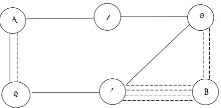
is too high, the process could become stuck at a local optimum. Overall simulated annealing needed longer computation times compared to the genetic algorithm. Meanwhile, Figure 3 shows the optimal solution for the system network planning using GA and SA.
7. NOTATION USED IN THE MODEL
CK Cost of generating a unit of power at bus-bar k.
EMi Maximum power flow of existing line i. K A large positive integer number.
LBE Number of basic loops containing existing lines only.
LBP Number of basic loops containing existing lines plus one proposed line. LE(l) Set of existing lines forming basic loop
)
(l which contains existing lines only. Lij Linearized cost coefficient representing
transmission losses cost of state j of proposed line i.
LP(l) Set of existing lines forming basic loop )
(l which contains one proposed line. MPK Minimum number of proposed line
connected to bus-bar k. NB Number of bus-bars.
NE Total number of existing lines. NG Set of generation bus-bars. NP Total number of proposed lines. NS(i) Number of states of proposed line i.
+
Ei
P Oriented power flow on existing line I from its "start" to its "end".
− Ei
P Oriented power flow on existing line I from its "end" to its "start".
Gk
P power generation at bus-bar k. +
ij
P Oriented power flow on state j of proposed line i from its "start" to its "end".
− ij
P Oriented power flow on state j of proposed line i from its "end" to its "start".
PLK Load at bus-bar k.
PMK Maximum power output of generator K. PMij Maximum power flow on state j of
proposed line i. '
Mij
P Minimum power flow on state j of proposed line i.
SE(k) Set of existing lines connected to bus-bar k.
Si Linearized cost coefficient representing transmission losses cost of existing line i. S(i) = k Set of lines that start form bus-bar k. SP(K) Set of proposed lines connected to
bus-bar k.
XEi Reactance of existing line i.
XPij Reactance of state j of proposed line i Z Total system cost (capital, transmission
losses, and generation). +
ij
Z Zero-one integer variable assigned to state j of proposed line i from its "start" to its "end".
− ij
Z Zero-one integer variable assigned to state
j
of proposed line i from its "end" to its "start".8. REFERENCES
1. Villasana, R., Garver, L. L. and Salon, S. J., “Transmission network planning using linear programming”, IEEE Trans. on PAS, Vol. PAS-104, No. 2, (Feb. 1985), 349-356.
2. Knight, U. G. W., “The logical design of electrical networks using linear programming methods”, Proc. IEE, Vol. 107A, No. 33, (1960), 306-319.
3. Garver, L. L., “Transmission network estimation using linear programming”, IEEE Trans. on PAS, Vol. PAS-89, No. 7, (Sep. - Oct. 1970), 1688-1697.
4. Serna, C., Duran, J. and Camargo, A., “A model for expansion planning of transmission systems: A practical application example”, IEEE Trans., Vol. PAS-97, No. 2, (1978), 610-615.
5. Berg, G. and Sharaf, T. A. M., “Reliability constrained transmission capacity assessment”, Electric Power Systems Research, Vol. 15, (1988), 7-13.
6. Kaltenbach, J. C., Peschon, J. and Gehring, E. H., “A mathematical optimization technique for the expansion of electric power transmission system”, IEEE Trans. on PAS, Vol. PAS-89, No. 1, (1970).
7. Farrag, M. A. and El - Metwally, M. M., “New method for transmission planning using mixed-integer programming”, IEEE Proc. C, Gen. Trans. and
5 1 4
6 2
3
Figure 3. Optimal network using genetic algorithm and
Distrib., Vol. 135, No. 4, (1988), 319-323.
8. Sharifnia, A. and Ashtiani, H. Z., “Transmission network planning: A method for synthesis of minimum - cost secure networks”, IEEE Trans. on PAS, Vol. PAS-104, No. 8, (1985).
9. Adams, R. N. and Laughton, M. A., “Optimal planning of power networks using mixed-integer programming”, IEEE Proc. C, Gen. Trans. and Distrib., Vol. 121, No. 2, (1974), 139-147.
10. Lee, T. V. and Hick, K. L., “Transmission expansion by branch - bound integer programming with optimal cost - capacity curves”, IEEE Trans. on PAS, Vol. PAS-93, No. 5, (1974).
11. Romero, R. and Monticelli, A., “A zero - one implicit enumeration method for optimizing investments in transmission expansion planning”, IEEE Trans. on PAS, Vol. 9, No. 3, (1994), 1385-1391.
12. Padiyar, K. R. and Shanbhag, R. S., “Comparison of methods for transmission system expansion using network flow and D. C. load flow models”, Electric power and energy systems, Vol. 10, No. 1, (1989), 17-24. 13. El-Metwally, M. M. and Al-Hamouz, Z. M.,
“Transmission network planning using quadratic programming”, Electric Machines and Power Systems, Vol. 18, No. 2, (1990), 137-148.
14. Youssef, H. K. and Hackam, R., “New transmission planning model”, IEEE Trans. on PAS, Vol. 4, No. 1, (Feb. 1989), 9-17.
15. El - Metwally, M. M. and Harb, A. M., “Transmission planning using admittance approach and quadratic programming”, Electric Machines and Power Systems, Vol. 21, (1993), 69-83.
16. El-Sobki, S. M., El-Metwally, M. M. and Farrag, M. A., “New approach for planning high-voltage transmission networks”, IEEE Proc., Vol. 133, No. 5, (1986), 256-262.
17. Albuyeh, F. and Skiles, J. J., “A transmission network planning method for comparatives studies”, IEEE Trans. on PAS, Vol. PAS-100, No. 4, (1981), 1679-1684.
18. Ekwue, A. O., “Investigations of the transmission system expansion problem”, Electric power and energy systems, Vol. 6, No. 3, (1984), 139-142.
19. Galiana, F. D., McGillis, D. T. and Marin, M. A., “Expert system in transmission planning”, Proc. IEEE, Vol. 80, No. 5, (1992), 712-726.
20. Yoshimoto, K., Yasuda, K. and Yokoyama, R., “Transmission expansion planning using neuro-computing hybridized with genetic algorithm”, Proc. 1995 IEEE Int. Conf. Evolutionary Computation, Perth, Australia, (1995), 126-131.
21. Romero, R., Gallego, R. A. and Monticelli, A. “Transmission system expansion planning by simulated annealing”, Proc. IEEE Power Industry Computer Application Conference (PICA’95), USA, (1995), 278-283.
22. Wen, F. and Chang, C. S., “Transmission network optimal planning using the tabu search method”, Electr. Power Syst. Res., Vol. 42, No. 2, (1997), 153-163. 23. Glover, F., Laguna, M., Taillard, E. and de Werra,
D., (Eds.), “Tabu search”, Science Publishers, Basel
Switzerland, (1993).
24. Glover, F., “Tabu search - part I”, ORSA J. Comput., Vol. 1, No. 3, (1989), 190-206.
25. Glover, F., “Tabu search - part II”, ORSA J. Comput., Vol. 2, No. 1, (1990), 4-32.
26. Bai, X. and Shahidehpour, S., “Hydro-thermal scheduling by tabu search and decomposition method”, IEEE PWRS, Vol. 11, No. 2, (1996), 968-974.
27. Wen, F. and Chang, C. S., “A tabu search approach to alarm processing in power systems”, IEE Proc. Generation, Transmission and Distribution, Vol. 144, No. 1, (1997), 31-38.
28. Bakirtzis, A., Petridis, V. and Kazarlis, S., “Genetic algorithm solution to the economic dispatch problem” IEEE Proc. - Gener. Trans. Distrib., Vol. 141, No. 4, (July 1994).
29. “Evolver user’s Guide”, Axcelis, Inc. Seattle, WA, USA, (2005).
30. Baker, J. E, “Adaptive selection methods for genetic algorithms”, In J. J. Grefenstette (Ed.), Proceedings of First International Conference on Genetic Algorithms, Erlbaum, (1985).
31. Davis, L., “Handbook of Genetic Algorithms”, Van Nostrand Reinhold, New York, (1991).
32. Goldberg, D. E., “Genetic algorithms in search optimization, and machine learning”, Addison Wesley, NY, (1989).
33. van Laarhoven, P. J. M. and Aarts, E. H. L., “Simulated annealing: Theory and applications”, Reidel, Dordrecht, Holland, (1987).
34. Tian, P. and Yang, Z., “An improved simulated annealing algorithm with genetic characteristics and traveling salesman problem”, Journal of Information and Optimization Sciences, Vol. 14, No. 3, (1993), 241-255.
35. Sadegheih, A., “Models in the iterative improvement and heuristic methods”, WSEAS Transactions on Advances in Engineering Education, Issue 4, Vol. 3, (April 2006), 256-261.
36. Sadegheih, A. and Drake, P. R., “Network optimization using linear programming and genetic algorithm”, Neural Network World, International Journal on Non - Standard Computing and Artificial Intelligence, Vol. 11, No. 3, (2001), 223-233.
37. Sadegheih, A., “Scheduling problem using genetic algorithm, simulated annealing and the effects of parameter values on GA performance”, Applied Mathematical Modeling, Issue 2, Vol. 30, (Feb. 2006), 147-154.
38. Sadegheih, A., “Design and implementation of network planning system”, 20th
International Power System Conf., Nov., Tehran, Iran, (2005), 14-16.
39. Sadegheih, A., “Modeling, simulation and optimization of network planning methods”, Proceeding of the WSEAS Int. Conference on Automatic Control, Modeling and Simulation, Prague, Czech Republic, (March 2006), 12-14.