A Wavelet Support Vector Machine Combination Model for Daily Suspended Sediment Forecasting

International Journal of Engineering

J o u r n a l H o m e p a g e : w w w . i j e . i r

A Wavelet Support Vector Machine Combination Model for Daily Suspended

Sediment Forecasting

M. SadeghpourHajia*_{, S. A. Mirbagheri}b_{, A. H. Javid}c_{, M. Khezri}a_{, G. D. Najafpour}d

a_{Department of Environmental Engineering, Faculty of Environment and Energy, Science and Research Branch, Islamic Azad University, Tehran, Iran} b_{Department of Civil and Environmental Engineering, K. N. Toosi University of Technology, Tehran, Iran}

c_{Islamic Azad university Tehran Science and Research Branch, Faculty of Marine Science and Technology, Tehran, Iran} d_{Biotechnology Research Center, Faculty of Chemical Engineering, BabolNoshirvani University of Technology, Babol, Iran}

P A P E R I N F O

Paper history:

Received 14September2013

Acceptedin revised form21November2013

Keywords:

Discrete Wavelet Analysis Support Vector Machine Daily Discharge Suspended Sediment

A B S T R A C T

In this study, wavelet support vector machine (WSWM) model is proposed for daily suspended sediment (SS) prediction. The WSVM model is achieved through combination of two methods; discrete wavelet analysis and support vector machine (SVM). The developed model was compared with single SVM. Daily discharge (Q) and SS data from YadkinRiver at Yadkin College, NC station in the USA were used. In order to evaluate the model, the root mean square error (RMSE), mean absolute error(MAE) and coefficient of determination (R2_{) were used.Results demonstrated that WSVM with RMSE =3294.6}

ton/day, MAE=795.22 ton/day and R2 _{=0.838 were more desired than the other model with RMSE}

=6719.7 ton/day, ton/day and R2_{=0.327. Comparisons of these models revealed that, MAE and error}

standard deviation for WSVM model were about 40% and 50% less than SVM model in test period.

doi:10.5829/idosi.ije.2014.27.06c.04

1. INTRODUCTION 1

Predicting daily, weekly and monthly, river suspended sediments are important components for operation of a water resource in hydrology and environmental engineering. Forecasting SS is not a simple task. It is difficult to project sediments. Extensive research was conducted to reduce the complexities of the discussed issue by developing practical methods that may not required dwelling on algorithm and theory. Thus, classical models such as multilayer regression (MLR) and sediment rating curves (SRCs) are widely used for suspended sediment modeling [1].

In recent years; special attentions have been focused on the use of artificial intelligence in the field of water resources and environmental issues. In this paper, literature provides several reliable methods for modeling river suspended sediment load such as artificial neural network (ANN), wavelet and SVM as discussed in the next paragraphs.

Artificial neural networks have created many applications in water resources and environmental

*Corresponding Author Email: [email protected]

(Maedeh Sadeghpour Haji)

engineering. Furthermore, wavelet analysis, owing to its attractive properties, has been recently discovered for the use of time series modeling. The wavelet-transformed data of observed time series improved the capacity of a prediction model by capturing useful information on various resolution levels [2]. Ability of ANNs to establish nonlinear links between inputs and outputs make them suitable tools for modeling hydraulic and hydrological phenomena [3].

ANN and neuro-fuzzy (NF) models were applied as effective methods to handle nonlinear and noisy data; especially in stations where the relationships among physical process were not fully understood.They were also particularly well matched for modeling multifaceted systems on real time basis.ANN, NF, MLR and SRC models were examinedfor simulation of suspended sediment in one dayahead in two hygrometry stations. For achievingsuch objectives, little Black River and Salt Riverstations in Missouri State in the USA were considered. Comparing the models results specified that the NF model had more ability in predicting SSC compared to other models[4].

gauging station in the USA [5]. In the developed model, daily observed time series of river discharge and suspended sediment were decomposed to some sub-time series. The reported data showed that the proposed model performed better than the NF and SRC models in prediction of suspended sediment [5].Hybrid WANN model was used for daily suspended sediment load forecast in Yadkin River at Yadkin College station in the USA. For SS simulation in the river, by the use of an effective characteristic of wavelet analysis, with the concepts of neural networks, a new wavelet artificial neural network model was developed. In order to obtain temporal properties of the input time series, the provided model, the discharge and SSL signals were primarily decomposed into sub-signals with different scales. The decomposed SS and Q time series were entered into the ANN technique for the prediction of SS in one day ahead. The comparison of prediction accuracies of the WANN and other models indicated that the proposed WANN model was successfully able to predict SS [6].Combined wavelet-ANN model was suggested for the prediction of suspended sediment load. Daily discharge and suspended sediment data derived from the Iowa River station in the United States were employed to train and test the ANN, WANN, MLR, and SRC models. Results indicated that the WANN model performed better than the other models in predicting extreme values of SS [7].

In another approaches, wavelet analysis and NF were applied to daily suspended sediment load prediction in a gauging station in the USA. In the WNF model, selection of appropriate decomposed time series was important in the model performance. Afterwards, these total time series were imposed as inputs into the NF model for SS prediction in one day ahead [8]. The support vector machine (SVM) was a supervised learning method that generates input-output mapping functions from a set of labeled training data [9]. In training support vector machines the decision boundaries were determined directly from the training data so that the separating margins of decision boundaries were maximized in the high-dimensional space called feature space. This learning strategy is based on statistical learning theory and minimizes the classification errors of the training data and the unknown data [10].

WSVR model has been investigated for forecasting daily precipitations and monthly stream flows. The WSVR models were developed by linking two methods, discrete wavelet transform and support vector regression. The WSVR models were tested with regards to different input combinations. The test results were compared with single support vector regression models. The comparison results specified that the WSVR performed better than the SVR in forecasting [11, 12]. SVM was used as a pattern-recognition (artificial intelligence) predictor to simulate daily, weekly and

monthly runoff and sediment yield from an Indian watershed [13]. In another survey, two input variable preprocessing methods for SVM model were explored, principal component analysis and the Gamma test. The proposed methods can provide more accurate performance on monthly stream flowforecasting[14]. Artificial neural network and support vector machine models were applied to predict suspended sediment load in Doiraj river basin situated in west of Iran [15].

Least square support vector machine (LSSVM) was compared with those of the artificial neural networks (ANNs) and sediment rating curve (SRC) in separate prediction of upstream and downstream station sediment data. The comparison results of the models showed that the LSSVM model commonly performed better than the ANN techniques. LSSVM and ANN models performed better than the SRC model for upstream station. However, for downstream station, SRC model was found to be better than the LSSVM and ANN models [16].Genetic programming (GP) technique was applied for estimating the daily suspended sediment load in two stations in Cumberland River in U.S. Results indicated that the GEP is superior to all of the other applied models in estimating suspended sediment load [17]. These surveys reveal that, wavelet transform is an operative procedure for precisely locating irregularly distributed multi-scale features of climate elements in space and times. The aim of combining the wavelet analysis and SVM technique is to improve the accuracy of SS prediction. Therefore, a WSVM model which uses multi-scale signals as input data may present more reliable predictions than a single pattern input.The purpose of the present work is combining LIBSVM and wavelet theory to forecast suspended sediments in river.

2. SUPPORT VECTOR MACHINE

Support vector regresses, which are extensions of support vector machines, have shown good generalization ability for various function approximation and time series prediction problems [10]. There are plenty of literatures which overview the theory of SVM [18, 19]. Therefore, only a brief explanation of a ε -SVM model, which is used in the present research, is stated. Suppose, we are giving training data

{

(

x₁,y₁

) (

,..., x_l,y_l

)

}

ÌX´R denote the space of the input patterns (e.g. X = Rd_{). In ε-SV}

regression has been conducted by Vapnik et al. for the prediction of the state model [20]. The aim of the present work is to find a function f(x)that has at most

εdeviation from the actual obtained targets yifor all the

Following equations describe the case of linear functions f, taking the form

R b X w with b x w x

f( )= , + Î , Î (1)

where _o,_o denotes the dot product in X. Flatnessin the case of Equation (1) means that one seeks a small w. One method to ensure thiswis minimizing the norm i.e.

w w

w2= , .We can write this problem as a convex optimization equation:

Minimize w2= w,w

Subject to

{

y_i - w,x_i -b£e (2)

The tacit theory in Equation (2) was that such a function

f actually exists that approximates all pairs (xi, yi) with ε

precision; the convex optimization problem is possible.We can present slack variables, _, *

i i e

e to cope

with otherwise infeasible constraints of the optimization problem in Equation (2). Therefore, we reached at the formulation specified in.

Minimize _å

(

)

= +

+ l

i i i

c

w2 ₁ *

2

1 _{d d}

Subject to ï ï î ï ï í ì ³ + £ -+ + £ -o * * , , , i i i i i i i i y b x w b x w y d d d e d e (3)

The constant C > 0 defines the trade-off between the flatness of f and the amount up to which deviations larger than ε are tolerated. This relates to deal with a so called ε–insensitive loss function d_e described by following expression: ïî ï í ì -< = otherwise if e d e d

d_e: 0 (4)

The optimization problem in Equation (3) can be solved more easily in its dual formulation.The main idea is to make a Lagrange function from the objective function (primal objective function) and the corresponding constraints, by introducing a dual set of variables. It can be presented that this function has a saddle point with respect to the primal and dual variables at the solution. We proceed as follows:

(

)

(

)

(

)

(

)

1

2 _{* * *}

1 1 1 * * 1 1 : 2 , , l

i i i i i i

i i

l

i i i i

i l

i i i i

i

L w c c

y w x b

y w x b

d d h d h d

a e d

a e d

= = = = = + + - + - + - + + - + + -

-å

å

å

å

(5)

Now L is the Lagrangian and _, *_{, ,} *

i i i

i h a a

h are

Lagrange multipliers. Therefore, the dual variables in Equation (5) have to satisfy positive constraint, i.e.

o ³ (*) (*)_, i i h

a .Remind that by (*)

i

a , we refer toai, ai(*).It

follows from the saddle point condition that the partial derivatives of L with respect to the primal variables

(

_{, , ,} *

)

i i b

w d d have to disappear for optimality. Equations

could be altered as follows:

(

)

(

)

* 1 * 1 , ( ) , l

i i i

i l

i i i

i

w x thus

f x w x b

a a a a = = = -= - +

å

å

(6)

This is the so-called Support Vector expansion, i.e. w

can be completely described as a linear combination of the training patterns xi. Moreover, note that the

comprehensive algorithm can be described in terms of dot products between the data. Even when evaluating

f(x), we do not need to compute w explicitly. These observations will be convenient for the formulation of a nonlinear extension. This, for instance, could be completed by only preprocessing the training patterns xi

by a map Φ: x →

Á

into some feature space

Á

and then applying the standard SV regression algorithm. As prior noted, the SV algorithm only depends on dot products between patterns xi.Therefore, it suffices to

know kernel function k(x,x'):= f(x),f(x') rather than

f explicitly. Moreover, note that in the nonlinear setting, the optimization problem associated with discovery of the flattest function in feature space, not in input space.The benefit of kernels is that, we do not need to treat the high dimensional feature space explicitly. This method is called kernel trick which is defined as follows:

(

*

)

(

)

1

( ) l _{i i} , '

i

f x a a k x x b

=

=

å

- + (7)

Various kernels that are used in support vector machines are linear kernels, polynomial kernels, radial basis function kernels and three-layer neural network kernels [20, 21].

3. DISCRETE WAVELET TRANSFORM

The theory of wavelet analysis was founded on the Fourier analysis. A signal is broken up flat sinusoids of limitless period in Fourier analysis. In wavelet technique, a signal is also broken up into wavelets, which are waveforms of efficiently limited duration and zero mean. Wavelet analysis is a windowing method with variable-sized areas. This analysis shows a time-scale view of a signal and delivers a method of expressing natural phenomena by employing their basic multi-fractal basis [22].

components improves the investigation of signals with localized impulses and oscillations. So, wavelet decomposition is perfect for considering transient signals and obtaining a superior characterization and more dependable discrimination technique [23]. The WT completes the decomposition of a signal into a group of functions:

(

jx k

)

x j jk

k

j, ( )=2 /2y , 2^

-y (8)

wherey_j,k is created from a mother wavelet y(x)which is dilated by j and translated by k. The mother wavelet has to please the condition.

The discrete wavelet function of a signal f(x) can be considered as follows:

òy(x)dx=o (9)

ò-¥¥

= f x x dx

cj,k ( )y*j,k( ) (10)

å

= _jkc_{jk jk} x

x

f( ) _, , y , ( ) (11)

where Cj,k is the approximate coefficient of a signal. The

mother wavelet is formulated from the scaling function

φ(x) as:

( )

å

-= h n x n

x) 2 ( ) 2

( j

j _o (12)

( )

å

-= h n x n

x) 2 ( ) 2

( 1 j

y (13)

where h1(n)=(-1)nho(1-n). Different sets of coefficients

o

h (n) could be equivalent to wavelet foundations with numerous characteristics. Coefficients h0(n) play a

serious character [6]. DWT drives two sets of function noticed as high-pass and low-pass filters. The original time series are passed through high-pass and low-pass filters and separated at different scales. The time series is decomposed into one comprising its trend (the approximation) and one comprising the high frequencies and the fast events (the details) [11].

4. CASE STUDY

In this research, we need uninterrupted time series data such as Q and SS. The data derived from the Yadkin River at Yadkin college, NC gauging station (USGS station No.: 02116500, basin area (sq. mi.): 2280, longitude: 080o _{23'10''and latitude: 035}o _{51'24'') in} Virginia State, operated by the U.S. Geological survey (USGS), were used for training and testing the employed models. In the present work, the data for a period of 30 years (01-October-1957 to 30-September-1987) were taken from the USGS web site. Data from October 1, 1957 to September 30, 1982 (25 years) and

the data from October 1, 1982 to September 30, 1987 (5 years) were used as training and testing sets, respectively. Figure 1 shows the time series of data related to daily Q and SS.

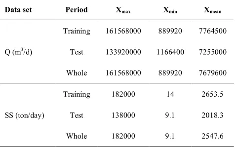
Table 1 signifies the statistical parameters of daily discharge and suspended sediment such as Xmax, Xmin and Xmean. It is obvious from the table that both discharge and sediment data display greatly scattered distribution.The attention of the first 25 years of the Q and SS time series for the calibration set has benefits; maximum experimental Q and SS happened through this period and considering important variations could be probable.

To qualify the correct selection of appropriate model input variables, the log-log autocorrelation and log-log cross-correlation between the Q and SS data were investigated. This method has been acceptably used for similar studies [5-8, 12, 16]. The log-log autocorrelation between SSt and SSt−4,t-5,…isquite low in test period; therefore, the model, whose inputs are the SS of four previous days was investigated. Various combinations of different lag time of SS and Q inputs that includes maximum four time steps into the past was selected.

Figure 1.Q and SS time series (30 years)

TABLE 1.Statistics investigation for training, testing and all data sets.

Data set Period Xmax Xmin Xmean

Q (m3_/d)

Training 161568000 889920 7764500

Test 133920000 1166400 7255000

Whole 161568000 889920 7679600

SS (ton/day)

Training 182000 14 2653.5

Test 138000 9.1 2018.3

Whole 182000 9.1 2547.6 0 1000 2000 3000 4000 5000 6000 7000 8000 9000 10000 11000 0

50,000,000 100,000,000 150,000,000 200,000,000

Time (day)

Q

(m

3/d)

0 1000 2000 3000 4000 5000 6000 7000 8000 9000 10000 11000 0

50,000 100,000 150,000 200,000

Time (day)

SS

(

ton

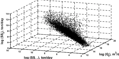
Figure 2.Logaritmic relationship between SSt, SSt-1, Qt.

The statistical parameters of stream flow (Qt) and SSCt, SSCt-1 are shown in Figure 2. It can be seen from

this figure that there is considerably highrelationship

between discharge and sediment data.Some

conventional evaluations such as correlation coefficient (ρ), coefficient of determination (R2_{), sum of square} error, and root mean square error (RMSE) were censoriously studied [24].

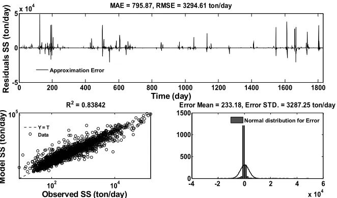
In this study, the performance of the models was evaluated employing R2_{, MAE and RMSE.The R}2_, which has a range of minus infinity to 1, with higher values describing superior agreement explains relation between observed and predicted values. RMSE estimates the residual between observed and predicted SS [25]. The models predictions are optimum if RMSE are found to be close to 0, respectively. For better judgment and visualization, the normal distributions for errors, mean of Error (Error mean) and Error Standard Deviation (Error STD) for SS could be calculated and illustrated. Normal distributions are symmetric and have bell-shaped density curves with a single peak and most of the samples in a set of data are close to the "average," though relatively few examples tend to one extreme or the other. While the examples are compactly gathered together and the bell-shaped curve is steep, the standard deviation is small. When the examples are spread apart and the bell curve is relatively flat it has a pretty large standard deviation. Different values of mean and standard deviation yield different normal density curves and hence different normal distributions. The standard deviation shows how tightly all the various examples are clustered around the mean in a set of data. The models predictions are optimum if RMSE, MAE, Error mean and Error STD are found to be close to 0, respectively. These equations are defined as follows:

( ) ( )

(

)

( ) ( )

(

)

2 1 2 1 1 n

i measured i predicted i

n

i measured i mean

i SS SS R SS SS = = =

-å

å

(14) ( ) ( ) 1 n

i measured i predicted

i SS SS

MAE

n

=

-=

å

(15)

( ) ( )

(

)

2

1 n

i measured i predicted

i SS SS

RMSE

n

=

-=

å

(16)

) ( )

(measured i predicted

i SS

SS

Errori = - ₍₁₇₎

( )

(

)

n Error Error ErrorSTD n

i i imean 2 1

å

=

-= (18)

In which n is the number of data points. A combined use of the mentioned measures will be adequate for model estimation.

5. APPLICATION AND RESULTS

In the present work, wavelet analysis was linked to

SVM technique for suspended sediment

simulation.They are also principally well suited for modeling nonlinear and noisy data on real time basis. Suspended sediment and river discharge time series were decomposed to some multi-frequently time series including details (different resolution levels) and approximation for each input variant.Then, decomposed SS and Q time series at different scales were used as inputs to the SVM method for predicting one-day-ahead SS. Appropriate mother wavelets was decomposed Q and SS, in different levels, from 1 to 4. For example, the level 2 decomposition of the Q signal that yields three subsignals by Daubechies2 wavelet is presented in Figure 3. In this figure, QApp is a discrete wavelet of Q in approximation mode and QDet1, QDet2 are discrete wavelets of SS at level 1 and 2. Although it is accepted that the SS at the future time step (SSt+1) is bound to be

a function of antecedent Q (Qt,t-1, t-2,…t-i) and antecedent

SS (SSt,t-1, t-2,…t-j) it is challenging to estimate

qualitatively how many time steps into the past would allow the greatest efficiency, the values of i and j are not known in advance [7].

Figure 3.Detail and approximation of sub-signals by

Daubechies2 wavelet (level 2)

12 14 16 18 20 2 4 6 8 10 12 142 4 6 8 10 12 14

log (Qt), m3/d log (SSt-1), ton/day

lo g ( SS t ), t o n /d ay

0 1000 2000 3000 4000 5000 6000 7000 8000 9000 10000 11000 -2

0 2x 10

8

Q

A

pp

0 1000 2000 3000 4000 5000 6000 7000 8000 9000 10000 11000 -1

0 1x 10

8

Q

D

et

1

0 1000 2000 3000 4000 5000 6000 7000 8000 9000 10000 11000 -1

0 1x 10

8

Q

D

et

Various combinations of inputs that include different lag time of SS and Q were tried for SVM and WSVM models and the finest one that provided the minimum RMSE error in test period was selected. Identifying best input combination is the most important step of any modeling.Following input combinations for the SS in one day ahead at time t+1 (SSt+1) were investigated:

1) Qt,Qt-₁,Qt-₂,Qt-₃,SSt,SSt-₁,SSt-₂, SSt-₃

2) Qt,Qt-₁,Qt-₂, SSt,SSt-₁,SSt-₂

3)Qt,Qt-₁,SSt,SSt-₁

4) Q_t,SS_t

5)Qt,SSt,SSt-₁

6) Qt,SSt,SSt-₁,SSt-₂,SSt-₃

7)Q_t,Q_t-1, SS_t,SS_t-1,SS_t-2,SS_t-3

Through learning by SVM the purpose is to discover a nonlinear function given by Equation (7) that minimizes a regularized risk function. This is achieved for the least value of desired error criterion (RMSE) for numerous constant parameter C and

e

,where C and

e

are two parameters which need to be specified in the application of SVM because if C is too small, then insufficient stress will be placed on fitting the training data and if C

is too large, then the algorithm will over fit the training data. If εis too large, then it will result in less support vectors. Therefore, the resulting regression model may yield large prediction errors on unobserved future data [26].In the paper, the radial base function (RBF) is used as the kernel function of e-SVM regression model for the following reason:

First, unlike the linear kernel, the RBF kernel can handle the case when the relation between class labels and attributes is non-linear. Second, the RBF kernels tend to give moral performance under general smoothness assumptions. Third, it has fewer tuning parameters than the polynomial and the sigmoid kernels [14]. Therefore, RBF kernel is chosen as the finest kernel for modeling. For non-linear systems such as SS prediction, determination of best input combination is a

difficult process.The parameter selection tool assumes that the RBF (Gaussian) kernel is used although extensions to other kernels and SVR can be easily made. The RBF kernel takes the form

( )

'2

'

,x e x x x

k = -g

-so (C,g ) are parameters to be decided [27].Building a SVM

-e model from training set requires values for C,

e

and g while using the RBF kernel function. Fine tuning of this variable can greatly improve the simplification capacity of the prediction system. The g value is significant in the RBF model and can lead to under fitting and over fitting in prediction. Under fitting happens when the models are incapable to predict the data that have been trained. Contrariwise, over fitting occurs when the models tend to memorize all the training data but are unable to generalize for unseen data; hence, only trained data points can be predicted [28]. The g parameter has a default value in LIBSVM software equal to 1/num-feature. In this research, the C

and

e

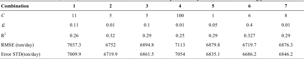
parameter is set to several values and various SVM models are developed.

Comparisons of the values of R2_{, RMSE, in test period} for the SVM model are listed in Table 2 and according to this table; the SVM model provided the best performance criteria for combination 6. In combination 6

(

Qt,SSt,SSt-₁,SSt-₂,SSt-₃

)

, the model with the C= 6 and e=0.4was chosen, which has the lowest RMSE value of 6719.17 ton/day and the highest R2 _{value of} 0.327.To define the periodic properties of the SS, the sub-signals achieved from wavelet transform are used as inputs to the WSVM model. The proposed model could be considered short, intermediate andlong levels by choosing appropriate decomposition levels for SS and Q time series.This model pre-processes the SS sub-time series and considers the effect of each signal. In this research different mother wavelets such as Meyer, Coiflets (Coif1), Daubechies (Db2), Haar (Haar 1), Symlets (sym 1) andBiorthogonal (Bior 1.1) were tested and the Db2 which is similar to SS signal, specially its peak was chosen.

TABLE 2. R2_{, RMSE, Error mean and Error STD values in SS prediction by SVM model in the testing period}

Combination 1 2 3 4 5 6 7

C 11 5 5 100 1 6 8

e

0.11 0.01 0.1 0.01 0.05 0.4 0.01

R2 _{0.26 0.32 0.29 0.25 0.29 0.327 0.29}

RMSE (ton/day) 7037.3 6752 6894.8 7113 6879.8 6719.7 6876.3

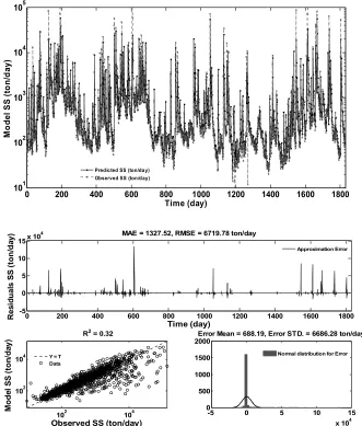
Figure 4.Daily suspended sediment forecasts of SVM model in testing period

0 200 400 600 800 1000 1200 1400 1600 1800

101

102

103

104

105

Time (day)

M

o

d

el

S

S

(t

o

n

/d

ay)

Predicted SS (ton/day) Observed SS (ton/day)

0 200 400 600 800 1000 1200 1400 1600 1800

-5 0 5 10 15x 10

4

Time (day)

R

es

id

u

al

s SS

(t

on

/d

ay)

MAE = 1327.52, RMSE = 6719.78 ton/day

Approximation Error

102 104

102 104

Observed SS (ton/day)

M

od

el

SS

(t

o

n

/d

ay)

R2 _{= 0.32}

Y = T Data

-5 0 5 10 15

x 104 0

500 1000 1500

2000Error Mean = 688.19, Error STD. = 6686.28 ton/day

Normal distribution for Error

0 200 400 600 800 1000 1200 1400 1600 1800

101 102 103 104 105

Time (day)

M

o

d

e

l SS

(t

on

/d

a

y)

Figure 5.Daily suspended sediment forecasts of WSVM model in testing period

The predictions done by the WSVM model, decomposed into 1 to 4 levels and when decomposition level increased more than 2; model’s performance decreased and led to small effectiveness. Becauseof an excessive number of factors with nonlinear relationship may be related to SVM technique.For this station, the relative RMSE and R2 _{for the SVM (input combination} 6) model are 6719.7 ton/day and 0.327 and the mentioned parameters are 3294.6 ton/day and 0.83 for the best WSVM (input combination 6) model in testing period. The values for C and

e

are considered 4 and 0.05 forthe best WSVM model and this model increased R2 _{almost 61% and reduced RMSE and MAE about} 40% and 51% in comparison to the best SVM model, respectively.The comparison of the results reveals that the WSVM may be considered as a proper model for this issue, though it is inferior to the simple-SVM. The SVM and WSVM forecast, and residuals for error are shown in Figures 4 and 5.Predictions by the proposed WSVM model are closer to the measured values than another model.SVM results were closer to the 1:1 line (45°) in the scatter plots in comparison with the other model. It is noticeable; the wavelet technique was significantly suitable to extract important features of SS signal. The results have shown that the advanced model could be an effective technique in SS forecasting. Comparisons of these two figures reveal that, error mean and error STD for WSVM model are about 66% and 50% less than SVM model in test period. In the developed model standard deviation is smaller than the other model. In SVM technique the examples are spread apart, hence the error standard deviation is 6686.28 ton/day. Wavelet and SVM model that is developed combining two procedures, DWT and SVM, appears to be more suitable than the single SVM model for forecasting daily SS. Complex hydro- l ogical

time-series are decomposed to different resolutions using DWT. Therefore, specific features of the sub-series could be seen more obviously than the original signal.

6. CONCLUSIONS

The aim of the present study is to investigate the accuracy of WSVM and SVM models for forecasting SS in one day ahead.The data on Yadkin River at Yadkin college NC gauging station in U.S for a period of 30 years (01-October-1957 to 30-September-1987) are taken from the USGS web site for training and testing.This research considered the potential of data driven process, in estimation of SS load. Q and SS time series were firstly decomposed into sub-signals with different scales by wavelet in order to find temporal properties of the input time series.Various combinations of inputs that include different lag time of SS and Q were tried for input of models. In the developed model,

the best WSVM model was used

3 2

1, ,

,

, t t- t- t

-t SS SS SS SS

Q as an independent variable,

which had the lowest RMSE value of 3294.6 ton/day and the highest R2_{value of 0.83. The comparison results} presented that the WSVM is superior to single SVM.

WSVM conjunction technique improved the

determination of coefficient with respect to the single SVM about 61% and reduced the root mean square errors 51%.

7. REFERENCES

1. Kisi, O., "Suspended sediment estimation using neuro-fuzzy and neural network approaches/Estimation des matières en

0 200 400 600 800 1000 1200 1400 1600 1800

-5 0 5x 10

4

Time (day)

R

es

id

u

a

ls

S

S

(

ton

/d

ay) MAE = 795.87, RMSE = 3294.61 ton/day

Approximation Error

102 104

105

Observed SS (ton/day)

M

od

el

S

S

(

ton

/d

ay)

R2 _{= 0.83842}

Y = T Data

-4 -2 0 2 4 6

x 104 0

500 1000

1500Error Mean = 233.18, Error STD. = 3287.25 ton/day

suspension par des approches neurofloues et à base de réseau de neurones",Hydrological Sciences Journal, Vol. 50, (2005) 2. Kim, T.-W. and Valdés, J.B., "Nonlinear model for drought

forecasting based on a conjunction of wavelet transforms and neural networks",Journal of Hydrologic Engineering, Vol. 8, (2003) 319-328.

3. Govindaraju, R.S., "Artificial neural networks in hydrology. II: hydrologic applications",Journal of Hydrologic Engineering, Vol. 5, (2000) 124-137.

4. Rajaee, T., Mirbagheri, S.A., Zounemat-Kermani, M. and Nourani, V., "Daily suspended sediment concentration simulation using ANN and neuro-fuzzy models",Science of the Total Environment, Vol. 407, (2009) 4916-4927.

5. Rajaee, T., "Wavelet and Neuro_‐fuzzy Conjunction Approach for Suspended Sediment Prediction",CLEAN–Soil, Air, Water, Vol. 38, (2010) 275-286.

6. Rajaee, T., "Wavelet and ANN combination model for prediction of daily suspended sediment load in rivers",Science of the Total Environment, Vol. 409, (2011) 2917-2928. 7. Rajaee, T., Nourani, V., Zounemat-Kermani, M. and Kisi, O.,

"River suspended sediment load prediction: Application of ANN and wavelet conjunction model",Journal of Hydrologic Engineering, Vol. 16, (2010) 613-627.

8. Rajaee, T., Mirbagheri, S., Nourani, V. and Alikhani, A., "Prediction of daily suspended sediment load using wavelet and neuro-fuzzy combined model",International Journal of Environmental Science Technology, Vol. 7, (2010) 93-110. 9. Wang, L., Support Vector Machines: theory and applications.

Springer, Vol. 177. (2005).

10. Abe, S., Support vector machines for pattern classification Springer, (2010)

11. Kisi, O. and Shiri, J., "Precipitation forecasting using wavelet-genetic programming and wavelet-neuro-fuzzy conjunction models",Water Resources Management, Vol. 25, (2011) 3135-3152.

12. Kisi, O. and Cimen, M., "A wavelet-support vector machine conjunction model for monthly streamflow forecasting",Journal of Hydrology, Vol. 399, (2011) 132-140.

13. Misra, D., Oommen, T., Agarwal, A., Mishra, S.K. and Thompson, A.M., "Application and analysis of support vector machine based simulation for runoff and sediment yield",Biosystems Engineering, Vol. 103, (2009) 527-535. 14. Noori, R., Karbassi, A., Moghaddamnia, A., Han, D.,

Zokaei-Ashtiani, M., Farokhnia, A. and Gousheh, M.G., "Assessment of input variables determination on the SVM model performance using PCA, Gamma test, and forward selection techniques for monthly stream flow prediction",Journal of Hydrology, Vol. 401, (2011) 177-189.

15. Kakaei Lafdani, E., Moghaddam Nia, A. and Ahmadi, A., "Daily Suspended Sediment Load Prediction Using Artificial Neural Networks and Support Vector Machines Machine",Journal of Hydrology, (2012)

16. Kisi, O., "Modeling discharge-suspended sediment relationship using least square support vector machine",Journal of Hydrology, Vol. 456, (2012) 110-120.

17. Kisi, O., Dailr, A.H., Cimen, M. and Shiri, J., "Suspended sediment modeling using genetic programming and soft computing techniques",Journal of Hydrology, Vol. 450, (2012) 48-58.

18. Theodoridis, S., Pikrakis, A., Koutroumbas, K. and Cavouras, D., Introduction to Pattern Recognition: A Matlab Approach: A Matlab Approach: Access Online via Elsevier. (2010)

19. Cherkassky, V. and Ma, Y., "Practical selection of SVM parameters and noise estimation for SVM regression",Neural Networks, Vol. 17, (2004) 113-126.

20. Vapnik, V., Golowich, S.E. and Smola, A., "Support vector method for function approximation, regression estimation, and signal processing",Advances in Neural Information Processing Systems, (1997) 281-287.

21. Smola, A.J. and Schölkopf, B., "A tutorial on support vector regression",Statistics and Computing, Vol. 14, (2004) 199-222. 22. Kucuk, M. and Ağirali-super, N., "Wavelet regression technique

for streamflow prediction",Journal of Applied Statistics, Vol. 33, (2006) 943-960.

23. Youssef, O.A., "A wavelet-based technique for discrimination between faults and magnetizing inrush currents in transformers",Power Delivery, IEEE Transactions on, Vol. 18, (2003) 170-176.

24. Legates, D.R. and McCabe, G.J., "Evaluating the use of

“goodness‐of‐fit” measures in hydrologic and hydroclimatic model validation",Water Resources Research, Vol. 35, (1999) 233-241.

25. Nash, J. and Sutcliffe, J., "River flow forecasting through conceptual models part I—A discussion of principles",Journal of Hydrology, Vol. 10, (1970) 282-290.

26. Xie, Z., Lou, I., Ung, W.K. and Mok, K.M., "Freshwater algal bloom prediction by support vector machine in macau storage reservoirs",Mathematical Problems in Engineering, (2012) 27. Chang, C.-C. and Lin, C.-J., "LIBSVM: a library for support

vector machines",ACM Transactions on Intelligent Systems and Technology (TIST), Vol. 2, (2011) 27.

A Wavelet Support Vector Machine Combination Model for Daily Suspended

Sediment Forecasting

M. SadeghpourHajia*_{, S. A. Mirbagheri}b_{, A. H. Javid}c_{, M. Khezri}a_{, G. D. Najafpour}d

a_{Department of Environmental Engineering, Faculty of Environment and Energy, Science and Research Branch, Islamic Azad University, Tehran, Iran} b_{Department of Civil and Environmental Engineering, K. N. Toosi University of Technology, Tehran, Iran}

c_{Islamic Azad university Tehran Science and Research Branch, Faculty of Marine Science and Technology, Tehran, Iran} d_{Biotechnology Research Center, Faculty of Chemical Engineering, BabolNoshirvani University of Technology, Babol, Iran}

P A P E R I N F O

Paper history:

Received 14 September 2013

Acceptedin revised form21 November2013

Keywords:

Discrete Wavelet Analysis Support Vector Machine Daily Discharge Suspended Sediment

هﺪﯿﮑﭼ

ﺖﺳاهﺪﺷهدﺎﻔﺘﺳانﺎﺒﯿﺘﺸﭘرادﺮﺑﻦﯿﺷﺎﻣﺎﺑﮏﺟﻮﻣيرﻮﺌﺗﺐﯿﮐﺮﺗزاﻖﯿﻘﺤﺗﻦﯾارد

.

رادﺮﺑﻦﯿﺷﺎﻣﺎﺑﻪﺘﻓﺎﯾﻪﻌﺳﻮﺗلﺪﻣﻦﯾا

ﺪﯾدﺮﮔﻪﺴﯾﺎﻘﻣنﺎﺒﯿﺘﺸﭘ

.

مﺎﮔوﺪﯾدﺮﮔهدﺎﻔﺘﺳاﺎﮑﯾﺮﻣآردﻦﯿﮐدﺎﯾﻪﻧﺎﺧدوريﺎﻫﺎﺘﯾدزا ﺎﻬﻧآﺐﯿﮐﺮﺗوبﻮﺳروﯽﺑدﻪﺘﺷﺬﮔيﺎﻫ

ﺪﺷهدادلﺎﻘﺘﻧالﺪﻣﻪﺑيدوروناﻮﻨﻋﻪﺑ

.

ﺺﺧﺎﺷﯽﺧﺮﺑزا ﺎﻄﺧﻖﻠﻄﻣرﺪﻗﻦﯿﮕﻧﺎﯿﻣﺮﯿﻈﻧيرﺎﻣآيﺎﻫ

)

MAE

(

ﻦﯿﯿﺒﺗﺐﯿﺑﺮﺿو

)

R2

(

ﺎﻄﺧتﺎﻌﺑﺮﻣﻦﯿﮕﻧﺎﯿﻣرﺬﺟو

)

(RMSE

ﺪﯾدﺮﮔهدﺎﻔﺘﺳالﺪﻣﯽﺑﺎﯾزراياﺮﺑ

.

ﮏﺟﻮﻣيرﻮﺌﺗﺐﯿﮐﺮﺗﻪﮐدادنﺎﺸﻧﺞﯾﺎﺘﻧ

ﺎﺑيﺮﺘﻬﺑﺞﯾﺎﺘﻧيارادنﺎﺒﯿﺘﺸﭘرادﺮﺑﻦﯿﺷﺎﻣﺎﺑ

ton/dayRMSE =3294.6 MAE=795.52 ton/day,

و

R2 _=0.838

ﺎﺑﯽﯾﺎﻬﻨﺗﻪﺑنﺎﺒﯿﺘﺸﭘرادﺮﺑﻦﯿﺷﺎﻣﻪﺑﺖﺒﺴﻧ

RMSE =6719.7ton/day, ton/dayMAE=1327.52

و

R2_=0.327

ﺪﺷﺎﺑ ﯽﻣ

.

ﮏﺟﻮﻣلﺪﻣ ردﺰﯿﻧ ﺎﻄﺧرﺎﯿﻌﻣ فاﺮﺤﻧا وﺎﻄﺧ ﻖﻠﻄﻣرﺪﻗ ﻦﯿﮕﻧﺎﯿﻣ

-ﻦﯿﺷﺎﻣ ﻪﺑ ﺖﺒﺴﻧنﺎﺒﯿﺘﺸﭘ رادﺮﺑ ﻦﯿﺷﺎﻣ

نﺎﺒﯿﺘﺸﭘرادﺮﺑ

40 %

و

50 %

دادنﺎﺸﻧﺶﻫﺎﮐ

.

doi:10.5829/idosi.ije.2014.27.06c.04