R E S E A R C H
Open Access
Oscillometric measurement of systolic and
diastolic blood pressures validated in a
physiologic mathematical model
Charles F Babbs
Correspondence:babbs@purdue.edu
Department of Basic Medical Sciences, Weldon School of Biomedical Engineering, Purdue University, 1426 Lynn Hall, West Lafayette, IN 47907-1246, USA
Abstract
Background:The oscillometric method of measuring blood pressure with an automated cuff yields valid estimates of mean pressure but questionable estimates of systolic and diastolic pressures. Existing algorithms are sensitive to differences in pulse pressure and artery stiffness. Some are closely guarded trade secrets. Accurate extraction of systolic and diastolic pressures from the envelope of cuff pressure oscillations remains an open problem in biomedical engineering.
Methods:A new analysis of relevant anatomy, physiology and physics reveals the mechanisms underlying the production of cuff pressure oscillations as well as a way to extract systolic and diastolic pressures from the envelope of oscillations in any individual subject. Stiffness characteristics of the compressed artery segment can be extracted from the envelope shape to create an individualized mathematical model. The model is tested with a matrix of possible systolic and diastolic pressure values, and the minimum least squares difference between observed and predicted envelope functions indicates the best fit choices of systolic and diastolic pressure within the test matrix.
Results:The model reproduces realistic cuff pressure oscillations. The regression procedure extracts systolic and diastolic pressures accurately in the face of varying pulse pressure and arterial stiffness. The root mean squared error in extracted systolic and diastolic pressures over a range of challenging test scenarios is 0.3 mmHg.
Conclusions:A new algorithm based on physics and physiology allows accurate extraction of systolic and diastolic pressures from cuff pressure oscillations in a way that can be validated, criticized, and updated in the public domain.
Background
The ejection of blood from the left ventricle of the heart into the aorta produces pulsatile blood pressure in arteries. Systolic blood pressure is the maximum pulsatile pressure and diastolic pressure is the minimum pulsatile pressure in the arteries, the minimum occur-ring just before the next ventricular contraction. Normal systolic/diastolic values are near 120/80 mmHg. Normal mean arterial pressure is about 95 mmHg [1].
Blood pressure is measured noninvasively by occluding a major artery (typically the brachial artery in the arm) with an external pneumatic cuff. When the pressure in the cuff is higher than the blood pressure inside the artery, the artery collapses. As the pres-sure in the external cuff is slowly decreased by venting through a bleed valve, cuff
pressure drops below systolic blood pressure, and blood will begin to spurt through the artery. These spurts cause the artery in the cuffed region to expand with each pulse and also cause the famous characteristic sounds called Korotkoff sounds. The pressure in the cuff when blood first passes through the cuffed region of the artery is an estimate of systolic pressure. The pressure in the cuff when blood first starts to flow continuously is an estimate of diastolic pressure. There are several ways to detect pulsatile blood flow as the cuff is deflated: palpation, auscultation over the artery with a stethoscope to hear the Korotkoff sounds, and recording cuff pressure oscillations. These correspond to the three main techniques for measuring blood pressure using a cuff [2].
In the palpatory method the appearance of a distal pulse indicates that cuff pressure has just fallen below systolic arterial pressure. In the auscultatory method the appear-ance of the Korotkoff sounds similarly denotes systolic pressure, and disappearappear-ance or muffling of the sounds denotes diastolic pressure. In the oscillometric method the cuff pressure is high pass filtered to extract the small oscillations at the cardiac frequency and the envelope of these oscillations is computed, for example as the area obtained by integrating each pulse [3]. These oscillations in cuff pressure increase in amplitude as cuff pressure falls between systolic and mean arterial pressure. The oscillations then de-crease in amplitude as cuff pressure falls below mean arterial pressure. The correspond-ing oscillation envelope function is interpreted by computer aided analysis to extract estimates of blood pressure.
The point of maximal oscillations corresponds closely to mean arterial pressure [4-6]. Points on the envelope corresponding to systolic and diastolic pressure, however, are less well established. Frequently a version of the maximum amplitude algorithm [7] is used to estimate systolic and diastolic pressure values. The point of maximal oscillations is used to divide the envelope into rising and falling phases. Then characteristic ratios or fractions of the peak amplitude are used to find points corresponding to systolic pressure on the rising phase of the envelope and to diastolic pressure on the falling phase of the envelope.
The characteristic ratios (also known as oscillation ratios or systolic and diastolic de-tection ratios [8]) have been obtained experimentally by measuring cuff oscillation amplitudes at independently determined systolic or diastolic points, divided by the maximum cuff oscillation amplitude. The systolic point is found at about 50% of the peak height on the rising phase of the envelope. The diastolic point is found at about 70 percent of the peak height on the falling phase of the envelope [7]. These empirical ratios are sensitive however to changes in physiological conditions, including most im-portantly the pulse pressure (systolic minus diastolic blood pressure) and the degree of arterial stiffness [9,10]. Moreover, a rational physical explanation for any particular ratio has been lacking. Since cuff pressure oscillations continue when cuff pressure falls be-neath diastolic blood pressure, the endpoint for diastolic pressure is indistinct. Most practical algorithms used in commercially available devices are closely guarded trade secrets that are not subject to independent critique and validation. Hence the best way to determine systolic and diastolic arterial pressures from cuff pressure oscillations remains an open scientific problem.
analysis of recorded cuff pressure oscillations to extract model parameters and predict the unique systolic and diastolic pressure levels that would produce the observed cuff pressure oscillations.
Methods Part 1: Modeling cuff pressure oscillations
Model of the cuff and arm
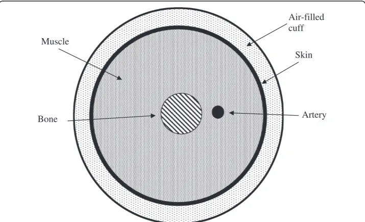
As shown in Figure 1, one can regard the cuff as an air filled balloon of dimensions on the order of 30 cm x 10 cm x 1 cm, which is wrapped in a non-expanding fabric around the arm. After inflation the outer wall of the cuff becomes rigid and the compli-ance of the cuff is entirely due to the air it contains. During an oscillometric run the cuff is inflated to a pressure well above systolic, say 150 to 200 mmHg, and then vented gradually at a bleed rate of r = 3 mmHg / second [11]. Small oscillations in cuff pressure happen when the artery fills and empties with blood as cuff pressure passes between systolic and diastolic pressure in the artery.
Let P0be the maximal inflation pressure of the cuff at the beginning of a run. The pressure is bled down slowly at rate, r mmHg/sec (about 3 mmHg/sec [11]). During the brief period of one heartbeat the amount of air inside the cuff is roughly constant. In addition to smooth cuff deflation, small cuff pressure oscillations are caused by pul-satile expansion of the artery and the corresponding compression of the air in the cuff. One can model the cuff as a pressure vessel having nearly fixed volume, V0 − ΔVa, where V0is cuff volume between heartbeats and ΔVa is the small incremental volume of blood in the artery beneath the cuff as it expands with the arterial pulse.
To compute cuff pressure oscillations from the volume changes,ΔVa, in the occluded artery segment it is necessary to know the compliance of the cuff, C =ΔV/ΔP, which is obtainable from Boyle’s law as follows. Boyle’s law is PV = nRT, where P is the absolute
Air-filled cuff
Skin Muscle
Bone Artery
pressure (760 mmHg plus cuff pressure with respect to atmospheric), V is the volume of air within the cuff, n is the number of moles of gas, R is the universal gas constant, and T is the absolute temperature. During the time of one heartbeat, n, R, and T are constants and n is roughly constant owing to the slow rate of cuff deflation. Hence to relate the change in cuff pressure,ΔP to the small change in cuff volume,ΔV, from ar-tery expansion we may writePV ðPþΔPÞ⋅ðVþΔVÞ PVþPΔVþVΔP, for abso-lute cuff pressure P. So
0PΔVþVΔP and Ccuff ¼ΔV ΔP ¼
ΔVa
ΔP
V0
P :
The negative change in cuff volume represents indentation by the expanding arm when the artery inside fills with blood. The effective cuff compliance, Ccuff , or more precisely the time-varying and pressure-varying dynamic compliance of the sealed air inside the cuff, is
Ccuff ¼dVcuff
dP ¼
V0
Pþ760mmHg;
with cuff pressure, P, expressed in normal clinical units of mmHg relative to atmos-pheric pressure. In turn, the time rate of change in cuff pressure is
dP
dt ¼ rþ 1 Ccuff
dVað Þt
dt ffi rþ
P0þ760rt
V0
dVað Þt
dt : ð1aÞ
In this problem as cuff pressure is slowly released, even as cuff volume remains nearly constant, the dynamic compliance of the cuff increases significantly and its stiffness decreases. Hence a suitably exact statement of the physics requires a differential equation (1a), rather than the constant compliance approximationP¼P0rtþVað Þt =Ccuff.
How-ever, equation (1a) may be integrated numerically to obtain a sufficiently exact representa-tion of cuff pressure changes with superimposed cardiogenic oscillarepresenta-tions.
Model of the artery segment
Next to characterize the time rate of volume expansion of the artery, dVa/dt, one can regard the artery as an elastic tube with a dynamic compliance, Ca, which varies with volume and with internal minus external pressure. The dynamic compliance Ca= dVa/d(Pa – Po), where Pt= Pa – Po is the transmural pressure or the difference between pressure inside the artery and outside the artery. Then
dVa dt ¼
dVa d Pað PoÞ⋅
d Pað PoÞ
dt ffiCa
dPa dt þr
; ð1bÞ
where the artery “feels” the prevailing difference between internal blood pressure and external cuff pressure, neglecting the small cuff pressure oscillations. The time derivative of arterial pressure can be determined from a characteristic blood pressure waveform and the known rate, r, of cuff deflation. Hence, the crucial variable to be specified next is the dynamic arterial compliance, Ca.
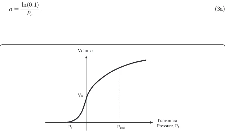
distending pressures. A few sources however [9,13] describe pressure-volume func-tions like the one sketched in Figure 2 for arteries subjected to both positive and negative distending pressure.
For classical biomaterials one can use two exponential functions to model the nonlinear volume vs. pressure relationship over a wide range of distending pressures. Here we shall use two exponential functions: one for negative pressure range and another for the posi-tive pressure range in a manner similar to that described by Jeon et al. [13]. The first expo-nential function for negative transmural pressure, Pt<0, is easy to imagine. For the negative transmural pressure domain artery volume Va ¼Va0eaPt for positive constant, a,
and zero pressure volume, Va0, of the artery. Here the dynamic compliance is clearly
dVa dPt ¼
aVa0eaPt for Pt<0: ð2aÞ
For the positive transmural pressure domain one can use a similar, but decelerating ex-ponential function [12]. However, there should be no discontinuity at the zero-transmural pressure point (0, V0). This means that for positive constant, b, and typically b < a,
dVa
dPt ¼aVa0e
bPt for P
t≥0: ð2bÞ
These two exponential functions can be used to characterize the dynamic compliance of the artery model in terms of easily obtained data, including the collapse pressure, Pc< 0, defined as the pressure when the artery volume is reduced to 0.1Va0 (for ex-ample, Pc=−20 mmHg) and the normal pressure arterial compliance, Cn, measured at normal mid-level arterial pressure, Pmid , halfway between systolic and diastolic pressure.
Solving for constant, a, we have
a¼ ln 0ð Þ:1
Pc : ð3aÞ
Transmural Pressure, Pt Volume
V0
Pc Pmid
Solving for constant, b, we have
b¼ ln Cn
aVa0
Pmid : ð
3bÞ
The zero pressure volume, Va0, can be known from anatomy if necessary, but as shown later is not needed if one is interested only in the relative amplitude of cuff pres-sure oscillations.
One can integrate the expressions (2a) and (2b) to obtain analytical volume versus pressure functions similar to Figure 2. Thus for Pt< 0
Va¼Va0þaVa0
Z Pt
0
eaPtdPt ¼Va
0eaPt; ð4aÞ
and for Pt≥0
Va ¼Va0þaVa0
Z Pt
0
ebPtdP
t
¼Va0
a bVa0 e
bPt 1
¼Va0 1þ
a b 1e
bPt
:
ð4bÞ
Figure 3 shows a plot of the resulting pressure-volume curve for a normal 10-cm long artery segment and constants a and b as described for initial conditions below. The form of the function is quite reasonable and consistent with prior work [9,13]. When bi-exponential constants a and b are varied, a wide variety of shapes for the pressure-volume curve can be represented. When pressure-volume changes more rapidly with pressure,
Figure 3Representative volume vs. pressure curves for an artery segment over a wide range of positive and negative transmural pressure.Standard normal variables a = 0.11 mmHg-1,
b = 0.03/mmHg-1, V
a0= 0.3 ml. Variations in shape occur with combinations of increased (2x normal) and
the artery is more compliant. When volume changes less rapidly with pressure, the ar-tery is stiffer. Increasing a and b in proportion allows greater volume change for a given pressure change and represents a more compliant artery. Decreasing a and b in propor-tion reduces the volume change for a given pressure change and represents a stiffer ar-tery. Increasing the ratio a/b represents a greater maximal distension. Decreasing the ratio a/b represents a smaller maximal distension.
Forcing function—the time domain blood pressure waveform
For proof of concept and validity testing one can use a Fourier series to represent blood pressure waveforms in these models [2]. A suitable and simple one for initial testing here is
Pa ¼DBPþ0:5PPþ0:36PP sinð Þ þωt 1
2sin 2ð ωtÞ þ 1
4 sin 3ð ωtÞ
ð5aÞ
for arterial pressure, Pa, as a function of time, t, withω being the angular frequency of the heartbeat, that isω= 2πf for cardiac frequency, f, in Hz. Here SBP is systolic blood pressure, DBP is diastolic blood pressure, and PP is pulse pressure (SBP−DBP). In turn, the derivative of the arterial pressure waveform is
dPa
dt ¼0:36ω cosð Þ þωt cos 2ð ωtÞ þ 3
4 cos 3ð ωtÞ
: ð5bÞ
Combining the cuff compliance, pressure-volume functions for the artery, and the ar-terial pressure waveform, one can write a set of equations for the rate of change in cuff pressure during an oscillometric pressure measurement in terms of P0, r, Va, Ccuff, and time. We must work with the time derivative of cuff pressure, rather than absolute cuff pressure, because the compliance of the cuff and also the form of the artery volume vs. pressure function vary with time and pressure during a run. Cuff pressure can then be computed numerically by integrating equation (1a),
dP
dt ffi rþ
P0þ760rt
V0
dVað Þt
dt : ð1aÞ
Using the chain rule of calculus, and taking transmural pressure as arterial blood pressure minus cuff pressure,
dVa
dt ¼aVa0e
a Pð aP0þrtÞ⋅ dPa dt þr
for PaP0þrt<0 ð6aÞ
dVa
dt ¼aVa0e
b Pð aP0þrtÞ⋅ dPa dt þr
for PaP0þrt≥0; ð6bÞ
with artery pressure, Pa, and its time derivative given by equations (5). Combining equations (1a) and (6) gives a precise model for cuff pressure oscillations.
Initial conditions
Artery dimensions:As a standard normal model consider a brachial artery with internal ra-dius of 0.1 cm under zero distending pressure. The resting artery volume is Va0=πr2L or
Stiffness constant a:For collapse to 10 percent at−20 mmHg transmural pressure we have
a¼ ln 0ð Þ:1
Pc ¼
2:3
20mmHg¼0:11mmHg
1:
Stiffness constant b: It is easy to estimate the normal pressure compliance of the bra-chial artery in humans, Cn, from experiments using ultrasound. For example, using the data of Mai and Insana [14], the brachial artery strain (Δr/r) during a normal pulse is 4 percent for a blood pressure of 130/70 mmHg with pulse pressure 60 mmHg. In turn the volume of expansion during a pulse is 2πrΔrL, where r is the radius and L is the length of the compressed artery segment. Hence for a normal pressure radius of 0.2 cm the change in volume would be
ΔVa¼6:28⋅0:2cm⋅0:04⋅0:2cm⋅10cm¼0:10cm3:
The normal pressure compliance for the artery segment is the volume change divided by pulse pressure or
Cn= 0.10 ml / 60 mmHg = 0.0016 ml/mmHg.
For normal artery the pressure halfway between systolic and diastolic pressure, Pmid, would be 100 mmHg, so
b¼
ln Cn aVa0
Pmid ¼
ln 0:0016 cm3 mmHg 0:11
mmHg⋅0:3cm
3
0 B B @
1 C C A
100mmHg ¼0:03 mmHg
1:
Jeon et al. [13] working with a similar model used a = 0.09 mmHg-1., b = 0.03 mmHg.
Numerical methods
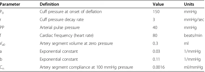
In this model equations (1), (5), and (6) govern the evolution of cuff pressure as a function of time during cuff deflation. Equation (1) can be integrated numerically using techniques such as the simple Euler method coded in Microsoft Visual Basic, Matlab, or“C”. In the results that follow cuff deflation is started from a maximal level of 150 mmHg and con-tinues over a period of 40 sec. Pressures are plotted every 1/20thsecond. To extract the small oscillations from the larger cuff pressure signal, as would be done in an automatic instrument by an analog high pass filter, cuff pressure at time, t, is subtracted from the average of pressures recorded between times t−Δt/2 and t +Δt/2 , whereΔt is the period of the pulse. For simplicity, filtered oscillations are not computed for time points that are Δt/2 seconds from the beginning or from the end of the time domain sample.
Methods Part 2: Interpreting cuff pressure oscillations
Artery motion during cuff deflation
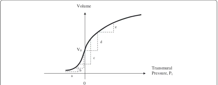
The shape of the volume vs. pressure curve for arteries determines the driving signal for cuff pressure oscillations during an oscillometric measurement, as shown in Figure 4.
The pulsatile component of transmural pressure causes the artery to change in vol-ume with each heartbeat. The magnitude of the change in transmural pressure is always equal to the pulse pressure (say, 40 mmHg) which is assumed to be constant during cuff deflation. As cuff pressure gradually decreases from well above systolic to well below diastolic pressure, the range of transmural pressure, Pt, experienced by the artery changes. At (a) cuff pressure is well above systolic and net distending pressure is always negative. There is a small change in arterial volume because the artery becomes less collapsed as each arterial pulse makes the transmural pressure less negative. As cuff pressure approaches systolic the relative unloading of negative pressure becomes more profound. Because of the exponential shape of the arterial pressure-volume curve, the amount of volume change accelerates. At (b) cuff pressure is close to systolic. After this point the volume change continues to increase but at a decelerating rate, because of the shape of the pressure-volume curve. Hence (b) is the inflection point for systolic pressure. At (c) cuff pressure is near mean arterial pressure and the volume change is maximal. At (d) cuff pressure is just below diastolic. After this point, as shown in (e), the volume change becomes less and less with each pulse as the increasingly distended artery becomes stiffer. Hence (d) is the inflection point for diastolic pressure. Thus the nonlinear compliance of arteries and the shape of the arterial pressure-volume curve govern the amplitude of cuff pressure oscillations.
The particular volume change of the artery from the nadir of diastolic pressure to the subsequent peak of systolic pressure can be specified analytically from Equations (4a) and (4b) as follows. Consider Ptas the transmural pressure at the diastolic nadir of the arterial blood pressure wave and let PP be the pulse pressure. One can imagine three domains of transmural pressure. In Domain (1) Pt+ PP < 0. In Domain (2) Pt< 0 and Pt+ PP≥0. In Do-main (3) Pt> 0. The largest artery volume oscillations occur in Domain (2) when transmural pressure oscillates between positive and negative values. Doman (1) represents the head of the oscillation envelope in time, and Domain (3) represents the tail.
Transmural Pressure, Pt Volume
V0
0 a
b c
d e
Using equations (4), the artery volume changes during the rising phase of the arterial pulse in each of the three domains are
Domain (1):
ΔVa¼Va0 ea PðtþPPÞeaPt
h i
ð7aÞ Domain (2):
ΔVa¼Va0 1þ
a b 1e
b Pð tþPPÞ
eaPt
h i
ð7bÞ
Domain (3):
ΔVa¼Va0
a b 1e
b PðtþPPÞ
a b 1e
bPt
h i
; ð7cÞ
where for cuff pressure, P, systolic blood pressure SBP, and diastolic blood pressure DBP, the transmural pressure Pt= DBP−P, and the pulse pressure PP = SBP−DBP.
It is easy to show by differentiating expressions (7) for Domains (1), (2), and (3) that the systolic and diastolic pressure points correspond exactly to the maximal and min-imal slopes d(ΔVa)/dPt. Therefore a simple analysis for finding systolic and diastolic pressures points would involve taking local slopes of the oscillation envelope vs. pres-sure function. Slope taking, however, is vulnerable to noise in practical applications. An alternative approach that does not involve slope taking creates a model of each individ-ual subject’s arm in terms of exponential constants a and b and then numerically finds the unique combination of systolic and diastolic arterial pressures that best reproduces the observed oscillation envelope.
Regression analysis for exponential constants
To obtain exponential constant, a, note that in the leading edge of the amplitude envelope at pressures near systolic blood pressure in Domain (1) the pulsatile change in cuff pressure is
ΔP¼ ΔVa Ccuff ¼
Va0
Ccuff e
a PðtþPPÞeaPt
h i
¼ Va0
Ccuff
ea PPð Þ1
h i
eaPt
¼ Va0
Ccuff
ea PPð Þ1
h i
ea DBPð PÞ
¼ Va0
Ccuff e
a PPð Þ1
h i
ea DBPð ÞeaP¼k
1eaP ð8Þ
for constant, k1, during a cuff deflation scan in which cuff pressure, P, varies and the other variables are constant. (Note that here Ccuffis very nearly constant because the rising phase of the pulse happens in a very short time, roughly 0.1 sec.) Hence, lnð Þ ¼ΔP lnð Þ k1 a P,
and a regression plot of the natural logarithm of the amplitude of pulse oscillations in the leading region of the envelope versus the instantaneous cuff pressure, P, yields a plot with slope−a. Thus we can obtain by linear regression an estimate of stiffness constant, a, as
^
a¼slope1. The range of the rising phase of the oscillation envelope from the beginning of
Similarly in Domain (3) during the tail region of the amplitude envelope at cuff pres-sures less than the maximal negative slope of the falling phase
ΔP¼ ΔVa Ccuff ¼
Va0
Ccuff a b 1e
b PðtþPPÞ
a b 1e
bPt
h i
¼ Va0
Ccuff a b 1þe
b PPð Þ
h i
ebPt
¼ Va0
Ccuff a b 1þe
b PPð Þ
h i
eb DBPð PÞ¼k3ebP ð9Þ
hence, lnð Þ ¼ΔP lnð Þ þk3 b P, and a regression plot of the natural logarithm of the
amplitude of pulse oscillations in the envelope tail versus cuff pressure at the time of each pulse yields a plot with slope b. In turn, we can obtain by linear regression an
esti-mate of stiffness constant, b, as^b¼slope3. The range of the falling phase of the
oscilla-tion envelope from the second inflecoscilla-tion point (maximal negative slope) of the oscillation envelope to the end of the envelope can be used to define the range of the second semi-log regression. More simply, the range of the falling phase of the oscilla-tion envelope from two thirds of the peak height to the end of the envelope provides reasonable estimates of slope3. The slope estimates from the head and tail regions of the amplitude envelope include multiple points and so are relatively noise resistant. Other variables involved in the lumped constants, k1and k3, are not relevant to the es-timation of exponential constants a and b.
Least squares analysis
Having estimated elastic constants a and b for a particular envelope of oscillations from a particular patient at a particular time, it is straightforward in a computer program to find SBP and DBP values that reproduce the observed envelope function most faithfully. Let y(P) be the observed envelope amplitude as a function of cuff pressure, P, and let ymax(Pmax) be the observed peak amplitude of oscillations at cuff pressure Pmax. Let^y(P, SBP, DBP) be the simulated envelope amplitude as a function of cuff pressure, P, for a particular pulse and a particular test set of systolic and diastolic pressure levels. The values of^yare obtained from equations (7) and the prevailing cuff compliance as follows
Domain (1):
^y¼ ΔVa
Ccuff ¼Va0 e
a SBPð PÞea DBPð PÞ
h i
⋅Pþ760
V0 ð
10aÞ
Domain (2):
^y¼ ΔVa Ccuff ¼
Va0 1þ
a b 1e
b SBPð PÞ
ea DBPð PÞt
h i
⋅Pþ760
V0 ð
10bÞ
Domain (3):
^y¼ ΔVa Ccuff ¼Va0
a b 1e
b SBPð PÞ
a b 1e
b DBPð PÞ
h i
⋅Pþ760
V0 : ð
10cÞ
oscillations for particular test values of SBP and DBP is the sum of squares over all measured pulses
SS SBPð ;DBPÞ ¼ X all pulses
y ymax
^
y
^ymax
2
: ð11Þ
The values of SBP and DBP that minimize this sum of squares are the taken as the best estimates of systolic and diastolic pressure by the oscillometric method.
Here cuff pressure, P, is the cuff pressure at the time of each oscillation. Use of the amplitude normalized ratios y/ymaxand^y/^ymax, means that it is not necessary to know the zero pressure volume of the artery, Va0, or cuff volume V0, which depend on anat-omy and geometry of a particular arm and cuff and are constants. It is the shape of the amplitude envelope in the pressure domain that contains the relevant information. The least squares function, SS, includes information from all of the measured oscillations and so is relatively noise resistant.
A variety of numerical methods may be used to find the unique values of SBP and DBP corresponding to the minimum sum of squares. Here, to demonstrate proof of concept, we evaluate the sum of squares, SS, over a two-dimensional matrix of candi-date systolic and diastolic pressures at 1 mmHg intervals and identify the minimum sum of squares by plotting. The values of SBP and DBP corresponding to this mini-mum sum of squares are the best fit estimates for a particular oscillometric pressure run. The best fit model takes into account the prevailing artery stiffness and also the prevailing pulse pressure.
Results and discussion Normal model
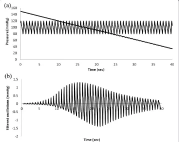
Particular parameter values for the standard normal model are as shown in Table 1. Figures 5 (a) and (b) show plots of cuff pressure and arterial pressure vs. time and high pass filtered cuff pressure oscillations vs. time. Figure 6 shows cuff pressure oscillations vs. cuff pressure and the amplitude envelope of cuff pressure for the standard normal model. Cuff pressure oscillations were obtained by subtracting each particular value from the moving average value over a period of one heartbeat.
Table 1 Standard parameters for the oscillometric blood pressure model
Parameter Definition Value Units
P0 Cuff pressure at onset of deflation 150 mmHg
r Cuff pressure decay rate 3 mmHg/sec
PP Arterial pulse pressure 40 mmHg
f Cardiac frequency (heart rate) 80 beats/min
Va0 Artery segment volume at zero pressure 0.3 ml
a Exponential constant 0.03 1/mmHg
b Exponential constant 0.11 1/mmHg
Varying arterial compliance
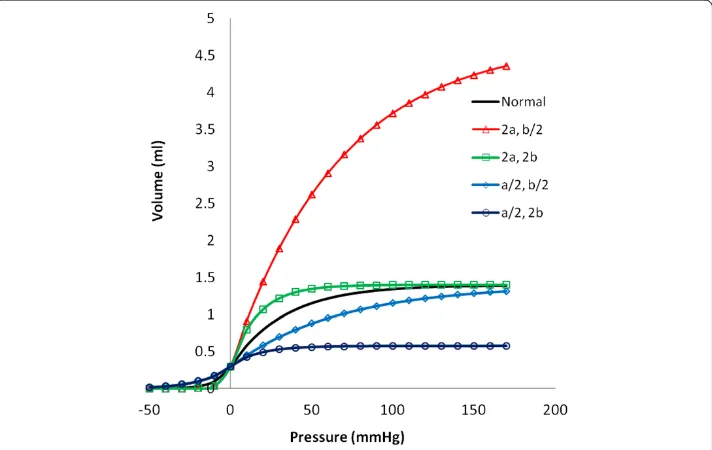
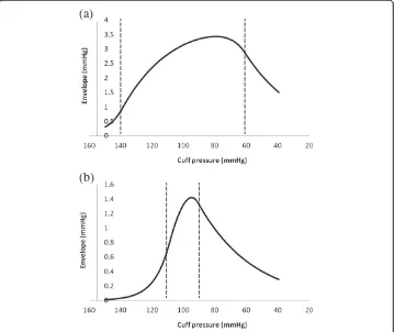
Prior studies have suggested that variations in arterial wall stiffness and arterial pulse pressure cause errors in systolic and diastolic blood pressure estimates using the oscil-lometric method [4,14,15]. Hence, these variables were studied explicitly. Figure 7 shows effects of varying arterial stiffness, represented by the constants a and b in the bi-exponential artery model. Actual blood pressure was 120/80 mmHg. The cuff oscil-lation ratios for systolic pressure are similar with varying stiffness. However, the cuff os-cillation ratios for diastolic pressure differ greatly among more compliant, normal, and stiffer arteries, indicating that the same oscillation ratios cannot be used to determine diastolic pressures from the amplitude envelope when artery stiffness varies. The dia-stolic oscillation ratios decrease from about 94% to 88% to 75% as stiffness decreases from high to normal to low. Oscillation amplitude ratios for diastolic pressure in par-ticular are highly dependent upon the stiffness of arteries. Since artery stiffness varies with age, this phenomenon may be a problem clinically. Note, however, that the max-imum and minmax-imum slopes of the envelope in the pressure domain still correlate well with true systolic and diastolic pressures.
Varying pulse pressure
Figures 8 and 9 show raw data and amplitude oscillation envelopes for cases of high and low pulse pressure. The amplitude of cuff pressure oscillations is greater for widened pulse pressure than for narrowed pulse pressure. The shape of the amplitude envelope is distorted for widened pulse pressure; however the maximum and minimum slopes of the
envelope in the pressure domain still correlate well with true systolic and diastolic pres-sures. Characteristic ratios for systolic and diastolic pressures vary with pulse pressure. The characteristic ratio for systolic pressure is substantially smaller for widened pulse pressure and significantly larger for narrowed pulse pressure. The characteristic ratio for diastolic pressure is substantially larger for widened pulse pressure than for narrowed pulse pressure.
Regression analysis for systolic and diastolic pressures
Figure 10 shows semi-log plots for the envelope functions shown in Figure 7 represent-ing arteries of varyrepresent-ing stiffness. The linear portions of the plots in the head and tail regions of log envelope amplitude vs. cuff pressure curves are evident. The artery stiff-ness constants a and b obtained from linear regression slopes for these head and tail regions are close to the nominal input values (data in Table 2).
Figure 11 shows a contour map of the sum of squares function in equation (11) for dif-ferent test values of systolic and diastolic blood pressure using the previously determined regression values for stiffness constants a and b. The semi-log regression slopes give
values for constants a and b of 0.1074 and 0.0303, respectively, versus the actual values of 0.110 and 0.030 used in the model to create the analyzed cuff pressure oscillations. The minimum sum of squares indicates the best fit between the oscillation envelope predicted by the mathematical model and the observed oscillation envelope. The minimum sum of
Figure 7Amplitude envelopes for varying arterial stiffness.Stiffness is represented as inverse compliance. Exponential constants a and b for 1/2 normal stiffness are multiplied by ln(2) = 1.44.
Exponential constants a and b for 2x normal stiffness are divided by 1.44. In all cases actual blood pressure was 120/80 mmHg.
squares is shown in Figure 11 as the center of the target-like pattern of colored, equal value contours. This point indicates the least squares solutions both for systolic pressure on the vertical scale and for diastolic pressure on the horizontal scale. Larger diameter ring-shaped contours indicate progressively greater sums of squares and therefore pro-gressively greater disagreement between observed and predicted oscillation envelopes. The contour interval is 0.1 dimensionless units. The flat background indicates exceedingly large, off-scale sums of squares > 1.5 units. The minimum sum of squares occurs for test values SBP/DBP of 119/80 mmHg. The actual pressure was 120/80 mmHg.
Figure 12 illustrates the sensitivity of the reconstruction algorithm to differences be-tween various test levels and the actual values of systolic and diastolic blood pressure, in this case 120/80 mmHg. A low value of test pressure (110/70) creates a reconstructed en-velope (dashed curve to left) that is clearly discordant with the observed normalized enve-lope values, E/Emax, shown as filled circles. A high value of test pressure (130/90) leads to equally discordant reconstructions in the opposite direction (heavy dashed curve to right). For both low and high test values the sum of squared differences is obviously large. The reconstructed model for the actual pressure (120/80) is shown as the solid curve. This il-lustration demonstrates the sensitivity of the least squares approach.
Validation of the regression procedure
The cuff-arm-artery model of an oscillometric pressure measurement described in Methods Part One can be used to validate the regression and analysis procedure of
(a)
(b)
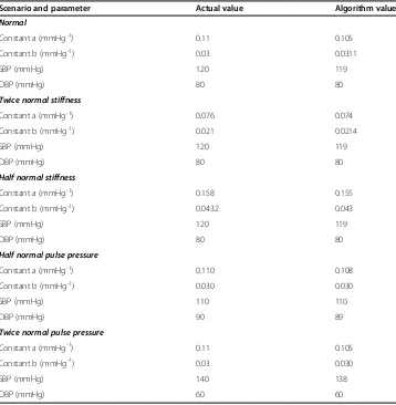
Figure 10Semi-log plots for determining model constants from amplitude envelope data.Note straight line regions in rising and falling phases of the curves.
Table 2 Validation of algorithm for estimation of systolic and diastolic pressures
Scenario and parameter Actual value Algorithm value
Normal
Constant a (mmHg-1) 0.11 0.105
Constant b (mmHg-1) 0.03 0.0311
SBP (mmHg) 120 119
DBP (mmHg) 80 80
Twice normal stiffness
Constant a (mmHg-1) 0.076 0.074
Constant b (mmHg-1) 0.021 0.0214
SBP (mmHg) 120 119
DBP (mmHg) 80 80
Half normal stiffness
Constant a (mmHg-1) 0.158 0.155
Constant b (mmHg-1) 0.0432 0.043
SBP (mmHg) 120 119
DBP (mmHg) 80 80
Half normal pulse pressure
Constant a (mmHg-1) 0.110 0.108
Constant b (mmHg-1) 0.030 0.030
SBP (mmHg) 110 110
DBP (mmHg) 90 89
Twice normal pulse pressure
Constant a (mmHg-1) 0.11 0.105
Constant b (mmHg-1) 0.03 0.030
SBP (mmHg) 140 138
Methods Part Two. An unlimited number and wide variety of test scenarios can be simulated in the model as unknowns for testing by the regression scheme, including a wide range of arterial stiffnesses and a wide range of pulse pressures, heart rates, blood pressure waveforms, cuff sizes, arm sizes, cuff lengths, artery diameters, etc. Import-antly, the regression analysis assumes no prior knowledge of these model parameters or of the blood pressure used to generate the simulated oscillations. Cuff pressure oscilla-tions and absolute cuff pressure are the only inputs to the algorithm for obtaining sys-tolic and diassys-tolic pressures.
The data summarized in Table 2 show the effectiveness of the proposed regression procedure in small sample of various possible test scenarios, including varying artery stiffness and varying pulse pressure. This small, systematic sample includes challenging cases for the algorithm. The accuracy is quite satisfactory, with reconstructed pressures within 0, 1, or 2 mmHg of the actual pressures in the face of varying artery stiffness and varying pulse pressure. The root mean squared error ispffiffiffi8=10 = 0.28 mmHg.
Discussion
The challenge of creating a satisfactory theoretical treatment of the genesis and inter-pretation of cuff pressure oscillations has attracted a diverse community of thinkers [4,5,7-10,16]. Nevertheless, specifying a valid method for extracting systolic and dia-stolic pressures from the envelope of cuff pressure oscillations remains an open prob-lem. Here is presented a mathematical model incorporating anatomy, physiology, and biomechanics of arteries that predicts cuff pressure oscillations produced during nonin-vasive measurements of blood pressure using the oscillometric method. Understanding of the underlying mechanisms leads to a model-based algorithm for deducing systolic
and diastolic pressures accurately from cuff pressure oscillations in the presence of varying arterial stiffness or varying pulse pressure.
The shape of the oscillation amplitude envelope dictates the stiffness parameters for the artery during both compression and distension. Semilog regression procedures give good estimates of the artery stiffness parameters that characterize each individual cuff deflation sequence. Using these parameters one can create and exercise an individua-lized cuff-arm-artery model for a wide range of possible systolic and diastolic pressures. The pair of systolic and diastolic pressures that best reproduces the observed oscillation envelope according to a least squares criterion constitutes the output of the algorithm.
When applied to amplitude normalized oscillation data the algorithm is insensitive to variations among subjects in zero pressure artery volume, Va0, or initial cuff volume V0, since these terms are constants that are eliminated by the normalization procedure. Compression of the entire length of artery underlying the cuff is not necessary. Incom-plete coupling of cuff pressure to the artery near the ends of the cuff merely decreases the ratio Va0/ V0without effecting the extracted systolic and diastolic pressures.
The cuff-arm-artery model can be used as well to test the validity of the algorithm for over a wide range of possible conditions by generating trial cuff pressure data for known arterial pressure waveforms. A stress test for the algorithm can be done by com-paring systolic and diastolic pressure levels extracted from synthesized cuff pressure oscillations with the arterial pressure that generated the synthesized oscillations over a wide range of test conditions. These conditions may include extreme cases that are hard to reproduce experimentally, contamination with excessive noise, any conceivable blood pressure waveforms, cardiac arrhythmias such as atrial fibrillation, etc. Such computational experiments, in addition to future animal and clinical studies, can boost confidence in the reliability of the oscillometric method and can suggest further refinements.
Here for convenience we have used the bi-exponential model to generate cuff pres-sure oscillations for algorithm testing. However, the regression algorithm does not
“know”where the sample data came from. It tries to extract constants a and b from the head and tail portions of the semi-log plot of oscillation amplitude versus cuff pressure. The resulting best fit values of a and b will still work for non-ideal or noise contami-nated data to produce a model envelope that can be matched to the actual data. An ex-tremely stiff artery with a linear pressure volume curve is easily accommodated by this process, since ex1 + x for small values of x. In this limiting case the exponential pressure-volume curve becomes linear. An exceptionally flabby artery, rather like dialy-sis tubing, is well described by larger values of a and b and a larger ratio a/b. Thus the family of bi-exponential models is very inclusive of a wide range of arterial mechanical properties, as suggested in Figure 3.
Classically the oscillometric method has been relatively well validated as a measure of mean arterial pressure, which is indicated by the peak of the oscillation amplitude envelope [4]. Automated oscillometric pressure monitors have found use in hospitals for critical care monitoring in which the goal is to detect any worrisome trend in blood pressure more so than the exact absolute value. Out of hospital use of the oscillometric method in screening for high blood pressure is more problematic, be-cause heretofore the accuracy of systolic and diastolic end points has been ques-tioned and doubted. For example Stork and Jilek [17] studied two published algorithms, differing in detail and based on cuff oscillation ratios of either 50% for systolic and 80% for diastolic or 40% for systolic and 55% for diastolic. Compared to a reference pressure of 122/78 mmHg the algorithmic methods applied to oscillo-metric data gave pressures of 135/88 and 144/81 mmHg, respectively. An advisory statement from the Council for High Blood Pressure Research, American Heart As-sociation [18] stressed the need for caution in the selection of all instruments used for blood pressure determination and the need for continuing studies to validate their the safety and reliability.
Accurate measurements of blood pressure in routine clinic and office settings are important because systemic arterial hypertension is a major cause of serious compli-cations, including accelerated atherosclerosis, heart attacks, strokes, kidney disease, and death. These serious complications increase smoothly with every point above the nominal 120/80 mmHg, hence even small increases in blood pressure are im-portant to detect. In screening for hypertension systematic bias or inaccuracy in blood pressure readings of a few mmHg can be significant, since the difference be-tween high normal (85 diastolic) and abnormal (90 diastolic) is only a few mmHg. A recent 1 million-patient meta-analysis suggests that a 3–4 mmHg increase in sys-tolic blood pressure would translate into 20% higher stroke mortality and a 12% higher mortality from ischemic heart disease [19].
Conclusions
The analytical approach and algorithm presented here represent a solution to an open problem in biomedical engineering: how to determine systolic and diastolic blood sures using the oscillometric method. Current algorithms for oscillometric blood pres-sure implemented in commercial devices may be quite valid but are closely held trade secrets and cannot be independently validated. The present paper provides a physically and physiologically reasonable approach in the public domain that can be independ-ently criticized, tested, and refined. Future demonstration of real-world accuracy will require data comparing oscillometric and intra-arterial pressures in human beings over a range of test conditions including variable cuff size, arm diameter, cuff tightness, cuff deflation rate, etc. Further development and incorporation of this algorithm into com-mercial devices may lead to greater confidence in the accuracy of systolic and diastolic pressure readings obtained by the oscillometric method and, in turn, an expanded role for these devices.
Competing interests
The author declares that he has no competing interests.
Author’s contributions
CB is the only author and is responsible for all aspects of the research and the intellectual and technical content of the manuscript.
Received: 28 June 2012 Accepted: 3 August 2012 Published: 22 August 2012
References
1. Boron WF, Boulpaep EL:Medical Physiology. 2nd edition. Philadelphia: Elsevier; 2005. 2. Geddes LA, Baker LE:Prinicples of Applied Biomedical Instrumentation. Second edition. 1975.
3. Soueidan K, Chen S, Dajani HR, Bolic M, Groza V:Augmented blood pressure measurement through the noninvasive estimation of physiological arterial pressure variability.Physiol Meas2012,33:881–899. 4. Mauck GW, Smith CR, Geddes LA, Bourland JD:The meaning of the point of maximum oscillations in cuff
pressure in the indirect measurement of blood pressure–part ii.J Biomech Eng1980,102:28–33.
5. Geddes LA, Voelz M, Combs C, Reiner D, Babbs CF:Characterization of the oscillometric method for measuring indirect blood pressure.Ann Biomed Eng1982,10:271–280.
6. Ursino M, Cristalli C:A mathematical study of some biomechanical factors affecting the oscillometric blood pressure measurement.IEEE Trans Biomed Eng1996,43:761–778.
7. Baker PD, Westenskow DR, Kuck K:Theoretical analysis of non-invasive oscillometric maximum amplitude algorithm for estimating mean blood pressure.Med Biol Eng Comput1997,35:271–278.
8. Drzewiecki G, Hood R, Apple H:Theory of the oscillometric maximum and the systolic and diastolic detection ratios.Ann Biomed Eng1994,22:88–96.
9. Forster FK, Turney D:Oscillometric determination of diastolic, mean and systolic blood pressure–a numerical model.J Biomech Eng1986,108:359–364.
10. van Popele N, Bos W, de Beer N, van der Kuip D, Hoffman A, Diederick E, CM W:Arterial stiffness as underlying mechanism of disagreement between oscillometric blood pressure monitor and sphygmomanometer.
Hypertension2000,36:484–488.
11. Pickering TG, Hall JE, Appel LJ, Falkner BE, Graves J, Hill MN, Jones DW, Kurtz T, Sheps SG, Roccella EJ: Recommendations for blood pressure measurement in humans and experimental animals: part 1: blood pressure measurement in humans: a statement for professionals from the Subcommittee of Professional and Public Education of the American Heart Association Council on High Blood Pressure Research.Circulation
2005,111:697–716.
12. Posey J, Geddes L:Measurement of the modulus of elasticity of the arterial wall.Cardiovasc Res Cent Bull1973, 11:83–103.
13. Jeon G, Jung J, Kim I, Jeon A, Yoon S, Son J, Kim J, Ye S, Ro J, Kim D, Kim C:A simulation for estimation of the blood pressure using arterial pressure-volume model.World Acad Sci Eng Technol2007,30:366–371. 14. Mai JJ, Insana MF:Strain imaging of internal deformation.Ultrasound Med Biol2002,28:1475–1484. 15. Ursino M, Cristalli C:Mathematical modeling of noninvasive blood pressure estimation techniques–Part I:
pressure transmission across the arm tissue.J Biomech Eng1995,117:107–116.
16. Ursino M, Cristalli C:Mathematical modeling of noninvasive blood pressure estimation techniques–Part II: brachial hemodynamics.J Biomech Eng1995,117:117–126.
17. Stork M, Jilek J:Cuff pressure waveforms: thier current and prospective application in biomedical
18. Jones DW, Frohlich ED, Grim CM, Grim CE, Taubert KA:Mercury sphygmomanometers should not be abandoned: an advisory statement from the Council for High Blood Pressure Research, American Heart Association.Hypertension2001,37:185–186.
19. Lewington S, Clarke R, Qizilbash N, Peto R, Collins R:Age-specific relevance of usual blood pressure to vascular mortality: a meta-analysis of individual data for one million adults in 61 prospective studies.Lancet2002, 360:1903–1913.
doi:10.1186/1475-925X-11-56
Cite this article as:Babbs:Oscillometric measurement of systolic and diastolic blood pressures validated in a physiologic mathematical model.BioMedical Engineering OnLine201211:56.
Submit your next manuscript to BioMed Central and take full advantage of:
• Convenient online submission
• Thorough peer review
• No space constraints or color figure charges
• Immediate publication on acceptance
• Inclusion in PubMed, CAS, Scopus and Google Scholar
• Research which is freely available for redistribution