R E S E A R C H
Open Access
Automated time activity classification based on
global positioning system (GPS) tracking data
Jun Wu
1,2*, Chengsheng Jiang
1, Douglas Houston
3, Dean Baker
4and Ralph Delfino
2Abstract
Background:Air pollution epidemiological studies are increasingly using global positioning system (GPS) to collect time-location data because they offer continuous tracking, high temporal resolution, and minimum reporting burden for participants. However, substantial uncertainties in the processing and classifying of raw GPS data create challenges for reliably characterizing time activity patterns. We developed and evaluated models to classify people’s major time activity patterns from continuous GPS tracking data.
Methods:We developed and evaluated two automated models to classify major time activity patterns (i.e., indoor, outdoor static, outdoor walking, and in-vehicle travel) based on GPS time activity data collected under free living conditions for 47 participants (N = 131 person-days) from the Harbor Communities Time Location Study (HCTLS) in 2008 and supplemental GPS data collected from three UC-Irvine research staff (N = 21 person-days) in 2010. Time activity patterns used for model development were manually classified by research staff using information from participant GPS recordings, activity logs, and follow-up interviews. We evaluated two models: (a) a rule-based model that developed user-defined rules based on time, speed, and spatial location, and (b) a random forest decision tree model.
Results:Indoor, outdoor static, outdoor walking and in-vehicle travel activities accounted for 82.7%, 6.1%, 3.2% and 7.2% of manually-classified time activities in the HCTLS dataset, respectively. The rule-based model classified indoor and vehicle travel periods reasonably well (Indoor: sensitivity > 91%, specificity > 80%, and precision > 96%; in-vehicle travel: sensitivity > 71%, specificity > 99%, and precision > 88%), but the performance was moderate for outdoor static and outdoor walking predictions. No striking differences in performance were observed between the rule-based and the random forest models. The random forest model was fast and easy to execute, but was likely less robust than the rule-based model under the condition of biased or poor quality training data.
Conclusions:Our models can successfully identify indoor and in-vehicle travel points from the raw GPS data, but challenges remain in developing models to distinguish outdoor static points and walking. Accurate training data are essential in developing reliable models in classifying time-activity patterns.
Background
Environmental air pollution has been associated with a variety of adverse health outcomes, including respiratory illness, cardiovascular diseases, pregnancy outcomes, and morbidity [1-5]. The knowledge of where individuals spend time is essential for human exposure assessment of air pollution because air pollutant concentrations may vary significantly by location. Studies have shown that traffic-generated air pollutants such as ultrafine par-ticles can be up to ten times higher inside a vehicle
compared to ambient outdoor concentrations because of proximity to vehicle exhaust [6-8]. Outdoor walking and cycling spaces often have lower concentrations of traf-fic-related pollutants than in-vehicle spaces [9], but often correspond with increased inhalation rates and longer travel durations which could result in a higher dose of air pollutant inhalation [10]. In addition, air pol-lutant concentrations can be much higher indoors than outdoors for pollutants with predominate indoor sources (e.g. environmental tobacco smoke) and vice versa for pollutants with predominate outdoor sources (e.g. ozone) [11,12]. Accurate characterization of people’s time-location patterns significantly reduce errors in * Correspondence: [email protected]
1Program in Public Health, University of California, Irvine, USA
Full list of author information is available at the end of the article
exposure estimates in environmental epidemiological studies in which personal exposure is not measured directly and has to be estimated.
Time activity data have traditionally been collected by recall telephone interviews or activity logs recorded by study participants [13,14]. However, these methods are limited by accuracy of recall, reliability, and compliance [15]. Recently, new techniques have been used to collect time-location data, such as the use of portable global positioning system (GPS) devices to track people’s time-location or commuting patterns with or without corre-sponding participant diary information [15-22]. GPS-based tracking presents an enormous opportunity for improving our understanding of the space-time activities of individuals and how they influence environmental exposure and health outcomes. It offers many advan-tages over traditional methods including near-continu-ous location tracking, high temporal resolution, and minimum reporting burden for participants [23]. How-ever, barriers exist for extracting accurate time activity patterns for human subjects from raw GPS data because they are not consistently reliable due to errors caused by satellite or receiver issues, atmospheric and iono-spheric disturbances, multipath signal reflection, or sig-nal loss or blocking [24]. The multipath problem occurs mainly in urban areas where tall buildings and struc-tures reflect satellite signals many times before they reach a GPS device, leading to GPS coordinate errors [25].
Since GPS datasets are usually very large (e.g., over 5,000 location coordinates per day at a 15-second inter-val) and are associated with such uncertainties, validated techniques are needed to automatically identify time activities in major microenvironments, such as commut-ing, indoor, and outdoor locations. The literature on GPS data classification techniques largely comes from the travel behavior and physical activity research fields. A number of studies have developed methods to classify travel activity using only GPS data or the combination of GPS and accelerometer data [26-34]. However, most of these studies collected data and developed models solely for travel activities (e.g. mode of travel, route choice, and distance traveled); some measurements were even conducted at predefined routes or activity sche-dules. Only a few studies have used GPS to track peo-ple’s time-activity patterns in free living conditions. Cho et al. [35] collected GPS and self-reported one-week location diary data for 5 research staff (35 person-days of data) for model development and calibration and 34 volunteers (136 person-days of data) for model valida-tion. They successfully developed and validated an algo-rithm to identify outdoor walking trips that lasted more than 5 minutes in free-living conditions. The authors reported difficulty in identifying walking trips with only
GPS information in free living conditions because peo-ple often walk very slowly or briskly and make short stops. Unfortunately, the application of the techniques used in these studies in air pollution epidemiological research is limited because people’s exposure to air pol-lution is significantly influenced by activity patterns across multiple indoor, outdoor, and transportation microenvironments. Few studies have evaluated techni-ques to classify people’s continuous time-activity pat-terns across both travel and non-travel periods based on GPS location data for subjects in free living conditions. To our knowledge, only one study by Adams et al. [36] developed an apportion algorithm for time-location pat-terns across indoor, outdoor and travel microenviron-ments based on data from a monitoring system that measured personal air pollution exposure, temperature, and real-time GPS locations. However, this study only tested the algorithm for a single person for four days with known home and workplace locations. In addition, their use of temperature to distinguish indoor from out-door locations in the winter of Colorado may not be applicable to other regions or seasons when indoor and outdoor temperature does not vary as much.
The purpose of this study was to address a major gap in the literature on air pollution epidemiology - the lack of reliable automated classification techniques to post-process multi-day GPS location tracking data for free living human subjects. We developed and evaluated two automated models that classify GPS tracking data into four major time-activity categories (i.e. indoor, outdoor static, outdoor walking, and in-vehicle travel) that are important in determining people’s exposure to traffic-related and other air pollutants [6-12].
Method
GPS and Roadway Data
reviewed over highly resolved and geographically recti-fied Digital Ortho Quarter Quads (DOQQ) aerial photo-graphy data from the United States Geological Survey using geographical information system (GIS) techniques in ArcGIS software (ESRI, Redlands, CA). Based on the participant logs and DOQQ imagery, prompts were gen-erated for follow-up interviews regarding discrepancies, unclear patterns, and suspected unreported activities. Follow-up interviews were administered 2-5 weeks after the monitored days because of the time required for post-processing GPS data and logistics. Based on feed-back from these interviews, the GPS data were finalized and coded into major location categories (e.g., indoor/ outdoor at home, school, restaurants, etc.) and travel mode (e.g., biking, walking, automobile, bus, train). Unfortunately these manually-classified data at times do not precisely differentiate indoor vs. near-building out-door points due to the positional error of GPS data [24]. In instances when it was not possible to consistently dis-tinguish near-building outdoor locations (e.g., patio and sidewalk) from indoor locations, participants were assumed to be indoors unless GPS locations were con-sistently separated from a building for at least 2-5 min-utes, in which case they were classified as outdoor.
Most (92.1%) of the HCTLS data were collected at a 15-second interval, while 4.0%, 0.1% and 3.8% of the data were collected at 1-second, 2 to 14 seconds, and > 15-second intervals, respectively. Since the recording intervals may occasionally shift even with a fixed interval setting in the GPS device, we decided to exclude only those points with no time stamp and data from one par-ticipant who had the majority of the data in 1-second interval. Data with speed higher than 200 kilometers per hour (km/h) (0.002% of all the data) were corrected to zero speed because they were determined through map-ping and follow-up interviews to be erroneous GPS locations which appeared far from the participant loca-tion and were caused by GPS device error or blocked satellite signals.
In addition to the HCTLS data, we collected 21 per-son-days of supplemental GPS time activity data for three UC-Irvine staff volunteers during December 6-13, 2010. The volunteers were asked to carry with them a GPS device (BT-Q1000XT from QSTARZ; approxi-mately 65 g; recording at a 15-second interval) and to record on a paper diary the following information: the start and end time for their major time activity patterns, mode of travel (outdoor walking or biking, in-vehicle travel by passenger car, bus, or train), and type of loca-tion including indoor or outdoor (home, work, school or education, other residence, park and recreational area, food-consumption related location, retailer store, short stops for gas-filling etc.). The BT-Q1000XT was used in this task mainly because it had longer battery
life (48 hours) than the DG-100 model used in the HCTLS (17 hours) [24]. Consistent with the manually-classified HCTLS data, these supplemental GPS data were manually classified based on the diary data, GIS verification, and verification by interview. The three staff volunteers were thoroughly instructed on how and when to record the diary logs and all of them were actively involved in the time activity research and knowledgeable of the study aims and possible mistakes that may be encountered by human participants.
There were two major differences between the HCTLS data and the supplemental UCI data. First, we obtained better diary logs in the supplemental dataset than the HCTLS study (particularly for the indoor vs. outdoor differentiation) because of more thorough and careful documentation of short-term events. The HCTLS only classified outdoor points as those that were consistently outdoors for at least 2-5 minutes based on map overlays in GIS software while the supplemental dataset recorded outdoor points at a much higher accuracy of less than 1 minute. In addition, slight differences were observed between the DG-100 used in the HCTLS and the Q1000x used in supplemental data collection; BT-Q1000x had a shorter acquisition time at cold start in an indoor environment, lower rate of data loss, but slightly poorer performance in spatial accuracy [24].
All GPS data were converted to the Universal Trans-verse Mercator projection (North American Datum NAD 83 and Zone 11 N). In addition to the above GPS data, we obtained roadway data for the study region from the ESRI StreetMap™ North America 9.3 http:// www.esri.com. This dataset was bundled with ArcGIS software products and included 2003 TeleAtlas® street data rather than the less-accurate TIGER 2000-based street data [38].
Model Development and Time-Activity Classifications We developed a rule-based model and a decision-tree based model to classify time-location patterns. The two types of models were chosen because the rule-based method best utilizes the user’s understanding of spatial patterns in the data (time, speed, and spatial relation-ships of the GPS points) while the decision-tree method requires minimal user-input and has been shown to out-perform the other approaches [32].
activities and were not examined in our models. No HCTLS participants traveled in an underground train; only 10 and 3 subjects reported bus travel and biking for a total of approximately 8 and 5 hours, respectively. No subway, bus, or biking activity was reported in the supplemental UCI data.
We did not distinguish indoor static vs. indoor moving conditions because the positional accuracy of GPS data was limited during indoor periods due to obstructed satellite signals from building structures. Our previous research indicates that the positional errors of the GPS devices can be large in typical indoor locations and can be in the range of 0-300 meters for DG-100 depending on the building materials (e.g., wood frame vs. concrete/ steel) and surrounding structures [24]. Significant GPS signal loss was also observed indoors in concrete struc-tures or strucstruc-tures surrounded by high buildings [24]. Therefore, we decided not to track participants’moving patterns in an indoor environment. Instead, we asked the study participants (≥21 years old) to place the GPS device on a static location (e.g., counter or desk) nearby while they were indoors at home, school, or work locations; thus most of our indoor data were static points.
Rule-Based Classification
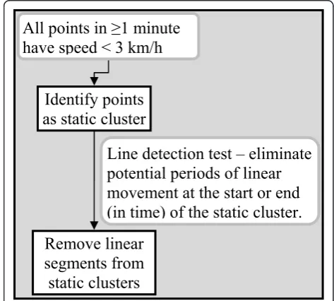
We developed the rule-based model using two open source software programs: R (version 2.10.1; R Founda-tion for Statistical Computing, Vienna, Austria) and PostgreSQL (version 8.4; PostgreSQL Global Develop-ment Group). The rule-based algorithm used three major features of the GPS data (i.e., time, speed, and spatial location) to classify GPS data to four major time activity categories: indoor, outdoor static, outdoor walk-ing, and in-vehicle travel (Figure 1). The rules were
developed based on logic and the summary statistics of the HCTLS data. For example, the model assumes that in-vehicle travel occurs on roadways and at higher aver-age speeds than outdoor walking and outdoor static conditions. Most of the threshold values were obtained from the summary statistics of each time-activity cate-gory in the HCTLS data.
First, we identified static clusters and moving periods based on continuity criteria in space and time. If all the points in a minimum of one minute had speed lower than 3 km/h, these points were treated as a static cluster (Figure 2). We further implemented a line detection process to identify the presence of linear alignment of sequential points which could indicate periods of move-ment within a static cluster. Starting from the first and last points of a cluster in time sequence, we selected three sequential points (moving forward in time from the first point and backward in time from the last point) to test if three consecutive points formed a linear seg-ment. The distance difference was calculated by sub-tracting (a) the distance from the first sequential point and the third sequential point from (b) the sum of the distance between the first sequential point and the ond sequential point and the distance between the sec-ond sequential point and the third sequential point. If the distance difference was no more than 1 m, we assumed that the three points formed a line and excluded them from the static cluster. This line detec-tion process proceeded through the sequence of points in each cluster until it detected three continuous points that did not form a line.
The second step in our rule-based classification was to identify sequential points which represent periods of
Raw GPS
data
Identify
static clusters
(Figure 2)
Identify
periods of
movement
(Figure 3)
Cleaned
GPS data
Differentiate
indoor from
outdoor static
points (Figure 5)
Differentiate
outdoor walking
from in-vehicle
travel (Figure 4)
Indoor
Outdoor
static
Outdoor
walking
In-vehicle
travel
Figure 1Overall flow chart.
Identify points
as static cluster
All points in
1 minute
have speed < 3 km/h
Line detection test – eliminate
potential periods of linear
movement at the start or end
(in time) of the static cluster.
Remove linear
segments from
static clusters
movement using the following criteria (Figure 3): 1) points with speed above 15 km/h; 2) a maximum of five sequential points bounded by two moving points identi-fied by step 1; 3) a minimum of six continuous points with speed above 2.5 km/h; 4) points within 10 m of a roadway but more than 25 m of the center of any static clusters; and 5) all other untagged points with speed more than 10 km/h. Adjacent moving periods were con-solidated into one if there was a single untagged point with at least two continuous moving points before and after this point or there were n (n≥2) continuous untagged points with a minimum of n continuous mov-ing points before and after them.
We further refined the moving classification by differ-entiating walking from in-vehicle travel periods using speed as a key parameter (Figure 4). A moving period was identified as in-vehicle travel if the second highest speed of the moving period was above 10 km/h and the median speed was above 5 km/h. We used a number of criteria to distinguish outdoor from indoor periods, including duration and time span of a static cluster, dis-tance between a static cluster and a participant’s home location, speed, the geographic range of the points in the cluster, and distance among critical points in the cluster (i.e. start, end, and middle point in time sequence) (Figure 5). The criteria were developed by analyzing the statistics of the manually-classified GPS data. For instance, we observed that indoor points occurred more often in static clusters that lasted longer (Additional file 1, Table S1), were closer to home, scat-tered somewhat more diversely (indicated as higher speed or wider geographic range of points), and showed
no apparent line pattern between sequential points. A home static cluster was roughly detected by checking whether the cluster included 12:00 AM or lasted for more than 24 hours, assuming that the participants
Classify the points as moving
5 sequential points bounded by two moving points with speed > 15 km/h Point with
speed > 15 km/h
Points within 10 m of a roadway but 25 m from the center of any static cluster
6 sequential points with speed >2.5 km/h
All un-tagged points with speed > 10 km/h
Identify moving periods Classify the points as moving
Check continuity in time for moving points
A single untagged point bounded by
2 continuous moving points at each end OR n (n2) sequential untagged points bounded by n continuous moving points at each end
Consolidate adjacent moving periods
Figure 3Identify periods of movement.
Moving period
The 2
ndhighest speed
>10 km/h and the
median speed > 5 km/h
Classify the points
as in-vehicle travel
Classify the
remaining points as
outdoor walking
Figure 4Differentiate outdoor walking from in-vehicle travel.
Yes No
Does the static cluster last >1 hour?b
Is the cluster close to homed?
Distance between the center of the cluster and home location < 50 m?f
Are there significant scattering? The 2nd lowest speed of all the
points in the cluster > 0.1 km/h?g
Is the range of points wide? Maximum range in either X or Y coordinate >30 m?h
Does the cluster last < 5 minutes?c
Yes No
Yes
No
No Yes
Yes Outdoor
Is an individual point in the cluster close to homed?
Distance between the point and home location <10 m?e
Yes
No No
Indoor
Does the static cluster include 12:00 AM or last >2 hour?a
Yes
No Indoor
Figure 5Differentiate indoor from outdoor static points.aWe
found that 99.5% of outdoor static clusters lasted less than 2 hours.
bAbout 2% (number) of outdoor static clusters (accounted for 21%
of the total outdoor static time) lasted 1-2 hours.cWe found 77% of
all the outdoor static clusters that satisfied the upper level rules (the rules above this criterion) lasted less than 5 minutes.dA home
were at their home under such conditions. We did not attempt to classify other types of locations (e.g. work, school, shopping) because without additional data we have to make many assumptions on the patterns of these activities, which may introduce a lot of uncertainties.
Random Forest Classification
As an alternative to the rule-based algorithm, we applied a machine learning model, random forest [42], to clas-sify the GPS data into different time activity categories. Here, a forest refers to a constellation of many decision tree models. Because a forest consists of many trees, it is more stable and less prone to prediction errors as a result of data perturbations [42]. Random forest is con-sidered one of the most accurate general-purpose learn-ing techniques available [43] and has been already widely used in bioinformatics [44,45]. Random forest creates multiple classification and regression (CART) trees, each trained on a bootstrap sample of the original training data and searches across a randomly selected subset of input variables to determine the split. Each tree in the forest gives or“votes”for a classification (e.g. time activity category). The forest chooses the classifica-tion having the most votes over all the trees in the forest.
In this study, we used an R interface in Waikato Environment for Knowledge Analysis (WEKA) 3.6 soft-ware, a popular machine learning workbench developed by researchers in University of Waikatoi [46,47]. We examined the following types of variables: acceleration rate, speed, distance difference, and distance ratio. Acceleration was calculated as the change in speed between a given point and the previous sequential point. The distance difference was calculated for any three sequential points as we described above for the rule-based model. The distance ratio was calculated for a ser-ies of sequential points as the ratio between (a) distance between the first sequential point and the last sequential point in the series and (b) the sum of the distance for all line segments formed by sequential points in the ser-ies. Speed, distance difference, and distance ratio vari-ables were calculated under various averaging time intervals ranging from 2 to 60 minutes and centered at each GPS point. Speed and distance difference were expressed as minimum, median, and maximum values. Standard deviation was also calculated for distance dif-ference. Final variables were selected by checking the variable importance index (a measure of the relative importance of the variables) generated from the model diagnostics and the correlations among the variables. We first selected 20 most important variables that were not highly correlated with each other (r < 0.75). Then we run the model again with these variables and
selected the most important variables with the p-value of the z-score < 0.001 for all the variables. Sensitivity tests were conducted for the maximum depth of a tree and the number of trees. Two separate models were developed based on the HCTLS data (hereafter HCTLS random forest model) and the supplemental UCI data (hereafter UCI random forest model). For both models, we randomly selected a subset of indoor points (N = 30,000 for the HCTLS data and N = 5,000 for the UCI data) in addition to all outdoor static, outdoor walking, and in-vehicle travel points in the original datasets as training data.
Model Evaluation
Time activity classifications of GPS data based on model predictions were compared to those from manually-clas-sified data for both the HCTLS and the supplemental datasets. There is no “gold-standard” against which to compare the classification of GPS-derived time activity data. In this study we used the manually-classified time activity classifications as the basis of model evaluation because these time activity codes were developed based on extensive quality assurance checks that involved careful inspection of real-time GPS locations in GIS using map overlays, comparison with participant activity logs, and clarifications from follow-up interviews with participants and staff. We examined the sensitivity (the ability of the model to identify specific cases), specificity (the ability of the model to identify non-cases), and pre-cision (the proportion of predicted cases that are cor-rectly real cases) of model prediction for each time activity category. Both the rule-based and the random forest models were evaluated against the HCTLS data and the supplemental UCI data. The two random forest models were evaluated using a repeated 10-fold cross validation method that has been recommended for model selection [48,49]. More specifically, the dataset was randomly split into 10 mutually exclusive subsets of equal size. The random forest model was trained on 9 subsets and validated on the remaining 1 subset of data; the procedure was repeated for 10 times. The reported validation results were the averages from the 10-folds testing. We further evaluated the capability of the ran-dom forest models in predicting new data by applying the HCTLS model to the UCI data and the UCI model to the HCTLS data.
Results
data, respectively, based on manually-classified time activity classifications. Based on the HCTLS data, the median duration of periods in each time activity cate-gory was 41, 2, 5, and 9 minutes for indoor, outdoor static, outdoor walking, and in-vehicle travel, respec-tively (Additional file 1, Table S1). The maximum dura-tion of the indoor clusters was 2.2 days (confirmed through our follow-up interview).
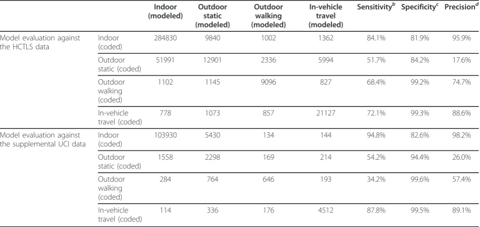
Table 1 shows classification results from the rule-based model. The rule-rule-based model classified indoor and in-vehicle travel points reasonably well for the HCTLS data (Indoor: sensitivity = 84%, specificity = 82%, and precision = 96%; in-vehicle travel: sensitivity = 72%, specificity = 99%, and precision = 89%). We observed moderate performance of the model on out-door static and outout-door walking predictions for the HCTLS data although the precision was very low for the outdoor static predictions (17.6%). For the supplemental UCI data, the model performed better for indoor, out-door static, and in-vehicle travel predictions, but worse for outdoor walking predictions. For both datasets, out-door static was the largest category of misclassifications for indoor, outdoor walking, and in-vehicle travel points, while most of the misclassification of outdoor static points was in the indoor category.
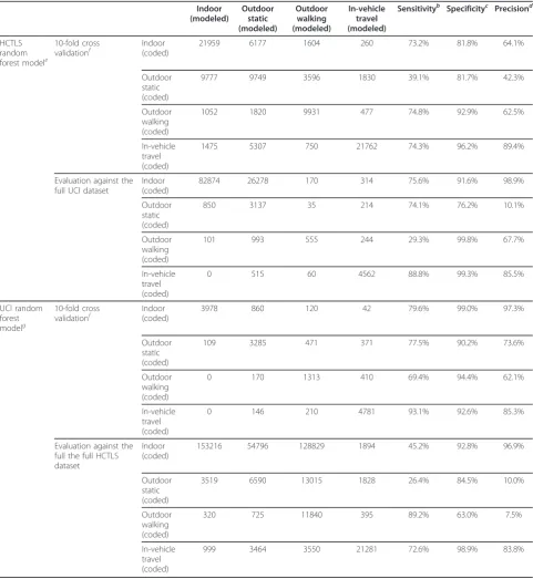
Table 2 shows classification results from the random forest models with ten trees with a maximum depth of three for each tree. Based on variable importance index and correlation analysis, we selected the following five
variables in the final models (by ranking of the variable importance index): maximum speed in 4 minutes, maxi-mum speed in 60 minutes, median speed in 30 minutes, maximum distance difference in 6 minutes, and maxi-mum distance difference in 30 minutes. Since the num-ber of predictor variables was small and little difference was found in the results of 10, 15, and 20 trees (unpub-lished data), we decided to report 10-tree model results in this paper. Sensitivity tests showed that the maximum depth of trees significantly influenced the model perfor-mance, particularly for the 10-fold cross validation results (Additional file 1, Table S2). No restrictions on the depth of the trees generated superb cross validation results with precision, specificity, and precision mea-sures all above 88% in the two random forest models (Additional file 1, Table S2). However, when the models were applied to predict new data (e.g. HCTLS model to predict UCI data and vice versa), the performance of the models degraded remarkably (Additional file 1, Table S2), likely due to model over-fit when the trees grow large. Therefore, we reported the results using a maxi-mum depth of three for each tree.
From the 10-fold cross validation results, we found similar performance of the random forest models com-pared to the rule-based model except somewhat degraded performance of the HCTLS model for indoor predictions and better performance of the UCI model for outdoor static and outdoor walking predictions. For new data prediction, the HCTLS model performed
Table 1 Time activity classification using the rule-based modela
Indoor (modeled)
Outdoor static (modeled)
Outdoor walking (modeled)
In-vehicle travel (modeled)
Sensitivityb Specificityc Precisiond
Model evaluation against the HCTLS data
Indoor (coded)
284830 9840 1002 1362 84.1% 81.9% 95.9%
Outdoor static (coded)
51991 12901 2336 5994 51.7% 84.2% 17.6%
Outdoor walking (coded)
1102 1145 9096 827 68.4% 99.2% 74.7%
In-vehicle travel (coded)
778 1073 857 21127 72.1% 99.3% 88.6%
Model evaluation against the supplemental UCI data
Indoor (coded)
103930 5430 134 144 94.8% 82.6% 98.2%
Outdoor static (coded)
1558 2298 169 214 54.2% 94.4% 26.0%
Outdoor walking (coded)
284 764 646 193 34.2% 99.6% 57.4%
In-vehicle travel (coded)
114 336 176 4512 87.8% 99.5% 89.1%
a
The rule-based model was developed based on logic and the summary statistics of manually-classified time activity classifications of HCTLS data.
b
Sensitivity was calculated as true positive estimation/(true positive estimation + false negative estimation).
c
Specificity was calculated as true negative estimation/(true negative estimation + false positive estimation).
d
Table 2 Time activity classification using the random forest modelsa
Indoor (modeled)
Outdoor static (modeled)
Outdoor walking (modeled)
In-vehicle travel (modeled)
Sensitivityb Specificityc Precisiond
HCTLS random forest modele
10-fold cross validationf
Indoor (coded)
21959 6177 1604 260 73.2% 81.8% 64.1%
Outdoor static (coded)
9777 9749 3596 1830 39.1% 81.7% 42.3%
Outdoor walking (coded)
1052 1820 9931 477 74.8% 92.9% 62.5%
In-vehicle travel (coded)
1475 5307 750 21762 74.3% 96.2% 89.4%
Evaluation against the full UCI dataset
Indoor (coded)
82874 26278 170 314 75.6% 91.6% 98.9%
Outdoor static (coded)
850 3137 35 214 74.1% 76.2% 10.1%
Outdoor walking (coded)
101 993 555 244 29.3% 99.8% 67.7%
In-vehicle travel (coded)
0 515 60 4562 88.8% 99.3% 85.5%
UCI random forest modelg
10-fold cross validationf
Indoor (coded)
3978 860 120 42 79.6% 99.0% 97.3%
Outdoor static (coded)
109 3285 471 371 77.5% 90.2% 73.6%
Outdoor walking (coded)
0 170 1313 410 69.4% 94.4% 62.1%
In-vehicle travel (coded)
0 146 210 4781 93.1% 92.6% 85.3%
Evaluation against the full the full HCTLS dataset
Indoor (coded)
153216 54796 128829 1894 45.2% 92.8% 96.9%
Outdoor static (coded)
3519 6590 13015 1828 26.4% 84.5% 10.0%
Outdoor walking (coded)
320 725 11840 395 89.2% 63.0% 7.5%
In-vehicle travel (coded)
999 3464 3550 21281 72.6% 98.9% 83.8%
a
The results reported here came from random forest models with 10 trees and a maximum depth of 3 for each tree.
b
Sensitivity was calculated as true positive estimation/(true positive estimation + false negative estimation).
c
Specificity was calculated as true negative estimation/(true negative estimation + false positive estimation).
d
Precision was calculated as true positive estimation/(true positive estimation + false positive estimation).
e
The model was developed based on all outdoor static, outdoor walking, in-vehicle travel and randomly selected 30,000 indoor points
f
The reported validation results were the averages from repeated 10-fold cross validation.
g
similarly as the rule-based model in predicting UCI data. However, the UCI model performed worse than the rule-based model in predicting HCTLS data, likely because of the very small and non-representative train-ing dataset for the development of the UCI model. Simi-lar to the rule-based model, we found that the HCTLS model most frequently misclassified indoor, outdoor walking, and in-vehicle travel to outdoor static while outdoor static to indoor category. The misclassification pattern was different for the UCI model, again likely due to the small and non-representative training data.
Discussion
We developed, evaluated, and compared two models to classify time-location patterns based solely on the pub-licly-available roadway data and raw GPS data (three-dimensional location data and the corresponding time stamps) from participants under free living conditions. To our knowledge, this is one of the first studies that developed models to systematically classify human time activity patterns for travel and non-travel activities based on raw GPS tracking data for use in air pollution epidemiological studies. Three major strengths of the study include the use of extensive manually-classified time-activity data from human participants under free living conditions for model development, the compari-son of two models in classifying time activity patterns, and additional model validation using supplemental data which were carefully collected and coded. The reason-ably good performance of the models indicates feasibility of using these models to reliably batch-process GPS tracking data from free living human subjects.
Air pollution epidemiological studies are increasingly using GPS to track time activity patterns of human sub-jects. However, few studies have used the GPS-derived time activity information extensively in exposure assess-ment and epidemiological analysis; rather, most prior studies rely on questionnaire-reported time activity pat-terns in the analysis. Lack of reliable methods to mine raw GPS data may be one of the major reasons for the limited and crude classification of these data. For instance, a Canadian study assigned all GPS points within 350 m of a residence as home and 400 m of a work place as work, and did not differentiate indoor from outdoor environments [50]; such an approach could lead to substantial exposure misclassification. A growing body of transportation and physical activity lit-erature has begun to provide insights into methods for automating the classification of GPS to identify different travel modes during periods of travel [26-34]. However, since our focus is to develop and evaluate procedures to classify GPS data for travel and non-travel periods given the paucity of applicable methods in the air pollution epidemiological literature, we do not provide a
comprehensive overview of the transportation and phy-sical activity literature.
Overall we found no striking differences in the perfor-mance of the rule-based model and the random forest models. Both models have advantages and disadvan-tages. The rule-based model features high flexibility and easy-to-interpret results, but the effort involved in the model development is substantial and may require a lot of additional data and resources. The random forest model is easy to use and requires minimum user inter-ference, but it faces a potential over-fitting problem if not properly trained and difficulty in results interpreta-tion. In terms of computational time, random forest was faster than the rule-based model (e.g. it took approxi-mately one hour for the rule-based model to predict the HCTLS data while < 30 seconds for the random forest to build the model for the same dataset on a 64-bit computer with 16 GB of memory and a 2.93 GB Intel® Core™ i7 Quad Core Processor). However, since ran-dom forest model is purely data driven, it may be more severely affected by biased or unrepresentative training data than the rule-based model. In fact, we observed poor model performance when the UCI random forest model was applied to predict the HCTLS data. With high quality training data, random forest model should be a good choice to quickly identify important predictor variables, develop exploratory models, or even final model based on its performance.
rule-based model would be improved if we refined classifica-tion rules using statistics from the UCI data because these data were limited to only three subjects who were indoors 87% of the time and had non-representative outdoor walking data. In addition, model performance may also be influenced by the different GPS devices used in the two dataset; however, we cannot determine this impact based on available data. We suggest avoiding the use of different GPS devices where a single time activity model is to be used for all of the GPS data.
We found that misclassifying between indoor and out-door static points was one of the most severe problems in both the rule-based and the random forest models. In Southern California, the majority of residential homes are wood structures that do not block satellite signals appreciably. In addition, for outdoor locations adjacent to buildings structures, GPS signals may be reflected by the buildings and result in positional error [24]. Because of the above reasons, the quality of the GPS data did not differ much between indoor and outdoor microen-vironments, which makes it difficult to differentiate the two under static conditions. Although we included the scatter patterns of the static clusters to differentiate indoor vs. outdoor static conditions (Figure 5), these measures did not do well as shown in our results. Out-door walking and in-vehicle travel were also frequently misclassified as outdoor static under low speed condi-tions (e.g., start or end of the trip near a static cluster). For in-vehicle travel, approximately 80% of the points that were wrongly classified as outdoor static points occurred when the participants stayed in the car without moving (e.g., waiting to pick up someone) or the car moved very slowly approaching or leaving a parking lot (results not shown). The models usually classified vehi-cle idling longer than two minutes or vehivehi-cle moving at very low speed as outdoor static, whereas participants usually reported such conditions as in-vehicle travel. One the other hand, we found that approximately 75% of the outdoor static points that were wrongly classified as in-vehicle travels lasted less than two minutes, indi-cating that this type of misclassification came from either coding errors (e.g., participants and research staff may have difficulty correctly reporting/coding the start or end of an in-vehicle travel period compared to an outdoor static period) or modeling errors (e.g., the mod-els were incapable of reliably classifying time activity categories near the start or end of an activity).
Three major limitations exist in this study. First, the manually-classified time activity classifications of the HCTLS and UCI data were not error free despite the extensive measures we have taken to minimize errors and enhance the accuracy of the coding (e.g., GPS track-ing was combined with a paper diary and in-person interview). Participants in the HCTLS tended to not
record short stops or trips such as walking to an adja-cent school to pick up a child from school or walking to a nearby corner store [37]. Although follow-up inter-views were used to clarify these discrepancies and to finalize the classifications of these missing periods, these data may not reliably capture the precise time of transi-tions between indoor and outdoor spaces particularly when participants lingered near a building entrance dur-ing the transition. Furthermore, even the most compli-ant participcompli-ants (including our research staff) may have difficulty correctly documenting the start and end time of an activity because it takes time and effort to record such information on a time activity log and this could interfere with ongoing activities.
The second limitation is that we collected data for 47 participants living in southern Los Angeles County and three staff volunteers living in Irvine, Orange County. Although the participants traveled throughout the region, , we did not target data collection for residents of areas with a more challenging built environment for GPS data collection, such as downtown Los Angeles where there are many tall and high-density buildings which our previous research indicates could result in more GPS signal loss and positional error [24]. Com-plete loss of satellite signals indoors, however, may not be a drawback because it can help determine whether people are indoors or outdoors. Future work is needed to refine the models so that they can classify time activ-ity patterns in a wide range of built environments.
The third limitation of the study is that our GPS-based time-activity patterns were not comprehensive enough for us to explore more refined time-activity pat-terns. For example, we had little GPS data for other modes of travel (e.g., bus, biking, and train). Future stu-dies should develop more refined classifications based on a combination of over-sampling of these travel modes and using related supplemental GIS data (e.g., trails and bus and train routes). In addition, we did not look at the impact of different GPS recording intervals on the model performance since the data were very lim-ited for the other time intervals. Only one subject had 1-second interval data (sometimes two seconds due to recording fluctuation); the fluctuation in GPS recordings at other intervals accounted for only about 3.9% of the data. We believe the rule-based model can be easily adjusted to accommodate different recording intervals.
number of satellites used in the determination of loca-tions, the number of satellites in view, and the dilution of precision which can influence satellite signal quality and positional accuracy. Our previous work has shown that horizontal dilution of precision was a good measure of spatial accuracy of the GPS data and may be helpful in distinguishing indoor vs. outdoor points [24]. Other studies have shown the number of satellites used in the location determination and the number of satellites in view can be used to improve classifications of GPS data [51]. However, our GPS data did not contain such infor-mation. Commercial POI data provide information on building and facility type (e.g. school, shopping, restau-rant, hospital, and park) and are available from a num-ber of companies (e.g., Garmin) with the main application being in GPS-based tracking and mapping software. Such POI data can help refine models to better classify different microenvironments (e.g. residence, school, restaurant) and time activity patterns (e.g. travel mode) and improve exposure assessment of air pollu-tants [27].
As we discussed above, this study was limited by input data quality (e.g. error in manually-classified time activ-ity classifications) and quantactiv-ity (e.g. lack of GPS diag-nostic and physical activity data). Despite the limitations, our models showed promising results in identifying time-location patterns in air pollution health studies where exposure levels vary remarkably by loca-tion (e.g. indoor, outdoor, and in-transit). With technol-ogy advances, the data quality and quantity will be improved significantly in the future research. For instance, some GPS devices (e.g. VGPS-900 from Visiontac™) can voice tag POI, which can improve the manually-classified time activity classifications. In addi-tion, certain physical activity monitors (e.g. GT3X+ activity monitor from ActiGraph™) records both activity level and ambient light - an intriguing parameter for distinguishing indoor vs. outdoor environment. In addi-tion to the ease of use and the minimal learning curve, the random forest model is capable of handling a large number (hundreds to thousands) of variables, which makes it a suitable modeling tool in future studies that may collect many types of measurement data in high temporal resolutions (e.g. GPS, actigraph, and electro-cardiogram data). With appropriate data, the model can be easily adapted to classify both time-location and phy-sical activity levels, which will advance the understand-ing of potential interactions between air pollution exposure and physical activity levels on health out-comes. In addition to air pollution epidemiology, the model can also be applied in other public health fields, such as physical activity and obesity research. More effort is needed to modify and validate the rule-based model before it can incorporate or classify other types
of data. But the rule-based model can be a good choice if the researchers have a good understanding of the data and if the decision tree approach cannot capture certain patterns in the data.
Conclusions
We successfully developed and evaluated two models to identify indoor and in-vehicle travel periods from raw GPS data under free living conditions. The rule-based model classified indoor and in-vehicle travel points rea-sonably well, but the performance was moderate for outdoor static and outdoor walking predictions. No striking differences were observed between the rule-based and the random forest models. The random forest model was fast and easy to execute, but was likely less robust than the rule-based model when the quality of the training data was poor.
Additional material
Additional file 1: Supplementary Material, Tables S1 and S2. Statistics of the duration of static clusters and periods of movement in each time activity category and results of sensitivity tests of maximum depth in the 10-tree random forest models.
Abbreviations
DOQQ: Digital orthophoto quarter quadrangle; GPS: Global positioning system.
Acknowledgements
The research was supported by the National Institute of Environmental Health Sciences (NIEHS, R21ES016379 and 3R21ES016379-02S1) and the National Children’s Study (Formative Research: LOI3-ENV-4-A #14 under Contract No. HHSN27555200503415). The HCTLS was supported by the California Air Resources Board (Contract No. 04-348) and the University of California Transportation Center. It would not have been possible without the HCTLS participants who generously allowed us to track their activities for multiple days. We also thank the staff volunteers who provided GPS time activity data and are grateful to the valuable insights and assistance provided by Lianfa Li, Paul Ong, Arthur Winer, Guillermo Jaimes, Walberto Martin, Jordan Simms and Carrie Ashendel.
Author details
1Program in Public Health, University of California, Irvine, USA.2Department
of Epidemiology, School of Medicine, University of California, Irvine, USA.
3Department of Planning, Policy and Design, School of Social Ecology,
University of California, Irvine, USA.4Center for Occupational &
Environmental Health, University of California, Irvine, USA.
Authors’Contributions
JW is the PI of this study. JW conceptualized the study, participated in study design, method development and data analysis, and drafted the manuscript. CJ conducted the modeling work and data analysis, and helped drafting the manuscript. DH provided the HCTLS GPS time activity dataset, reviewed the manuscript, and revised it critically for important intellectual content. DB and RD helped conceptualize the study and provided important intellectual content for the manuscript. All authors assisted in the interpretation of results and contributed towards the final version of the manuscript. All authors read and approved the final manuscript.
Competing interests
Received: 7 June 2011 Accepted: 14 November 2011 Published: 14 November 2011
References
1. Brook RD:Is air pollution a cause of cardiovascular disease? Updated review and controversies.Rev Environ Health2007,22:115-137. 2. Chen H, Goldberg MS, Villeneuve PJ:A systematic review of the relation
between long-term exposure to ambient air pollution and chronic diseases.Rev Environ Health2008,23:243-297.
3. Englert N:Fine particles and human health–a review of epidemiological studies.Toxicol Lett2004,149:235-242.
4. Pelucchi C, Negri E, Gallus S, Boffetta P, Tramacere I, La Vecchia C: Long-term particulate matter exposure and mortality: a review of European epidemiological studies.BMC Public Health2009,9:453.
5. Stillerman KP, Mattison DR, Giudice LC, Woodruff TJ:Environmental exposures and adverse pregnancy outcomes: a review of the science.
Reprod Sci2008,15:631-650.
6. Chan CC, Ozkaynak H, Spengler JD, Sheldon L:Driver Exposure to Volatile Organic-Compounds, Co, Ozone, and No2 under Different Driving Conditions.Environmental Science & Technology1991,25:964-972. 7. Zhu Y, Eiguren-Fernandez A, Hinds WC, Miguel AH:In-Cabin Commuter
Exposure to Ultrafine Particles on Los Angeles Freeways.Environ Sci Technol2007,41:2138-2145.
8. Westerdahl D, Fruin S, Sax T, Fine PM, Sioutas C:Mobile platform measurements of ultrafine particles and associated pollutant concentrations on freeways and residential streets in Los Angeles.
Atmospheric Environment2005,39:3597-3610.
9. Briggs DJ, de Hoogh K, Morris C, Gulliver J:Effects of travel mode on exposures to particulate air pollution.Environ Int2008,34:12-22. 10. de Nazelle A, Nieuwenhuijsen MJ, Anto JM, Brauer M, Briggs D,
Braun-Fahrlander C, Cavill N, Cooper AR, Desqueyroux H, Fruin S, Hoek G, Panis LI, Janssen N, Jerrett M, Joffe M, Andersen ZJ, van Kempen E, Kingham S, Kubesch N, Leyden KM, Marshall JD, Matamala J, Mellios G, Mendez M, Nassif H, Ogilvie D, Peiro R, Perez K, Rabl A, Ragettli M,et al:Improving health through policies that promote active travel: a review of evidence to support integrated health impact assessment.Environ Int2011,
37:766-777.
11. Weisel CP, Zhang J, Turpin BJ, Morandi MT, Colome S, Stock TH, Spektor DM, Korn L, Winer AM, Kwon J, Meng QY, Zhang L, Harrington R, Liu W, Reff A, Lee JH, Alimokhtari S, Mohan K, Shendell D, Jones J, Farrar L, Maberti S, Fan T:Relationships of Indoor, Outdoor, and Personal Air (RIOPA). Part I. Collection methods and descriptive analyses.Res Rep Health Eff Inst2005, 1-107, discussion 109-127.
12. Suh HH, Bahadori T, Vallarino J, Spengler JD:Criteria air pollutants and toxic air pollutants.Environ Health Perspect2000,108(Suppl 4):625-633. 13. Wallace L, Nelson W, Ziegenfus R, Pellizzari E, Michael L, Whitmore R,
Zelon H, Hartwell T, Perritt R, Westerdahl D:The Los Angeles TEAM study: personal exposures, indoor-outdoor air concentrations, and breath concentrations of 25 volatile organic compounds.J Expos Anal Environ Epidemiol1991,1:157-192.
14. Klepeis NE, Nelson WC, Ott WR, Robinson JP, Tsang AM, Switzer P, Behar JV, Hern SC, Engelmann WH:The National Human Activity Pattern Survey (NHAPS): a resource for assessing exposure to environmental pollutants.
Journal of Exposure Analysis and Environmental Epidemiology2001,
11:231-252.
15. Elgethun K, Yost MG, Fitzpatrick CTE, Nyerges TL, Fenske RA:Comparison of global positioning system (GPS) tracking and parent-report diaries to characterize children’s time-location patterns.Journal of Exposure Science and Environmental Epidemiology2007,17:196-206.
16. Duncan MJ, Mummery WK:GIS or GPS? A comparison of two methods for assessing route taken during active transport.American Journal of Preventive Medicine2007,33:51-53.
17. Elgethun K, Fenske RA, Yost MG, Palcisko GJ:Time-location analysis for exposure assessment studies of children using a novel global positioning system instrument.Environmental Health Perspectives2003,
111:115-122.
18. Schantz P, Stigell E:A Criterion Method for Measuring Route Distance in Physically Active Commuting.Medicine and Science in Sports and Exercise
2009,41:472-478.
19. Rainham D, Krewski D, McDowell I, Sawada M, Liekens B:Development of a wearable global positioning system for place and health research.
International Journal of Health Geographics2008,7:59.
20. Phillips ML, Hall TA, Esmen NA, Lynch R, Johnson DL:Use of global positioning system technology to track subject’s location during environmental exposure sampling.Journal of Exposure Analysis and Environmental Epidemiology2001,11:207-215.
21. Larsson P, Henriksson-Larsen K:The use of dGPS and simultaneous metabolic measurements during orienteering.Medicine and Science in Sports and Exercise2001,33:1919-1924.
22. Stopher P, FitzGerald C, Zhang J:Search for a global positioning system device to measure person travel.Transportation Research Part C-Emerging Technologies2008,16:350-369.
23. Rainham D, McDowell I, Krewski D, Sawada M:Conceptualizing the healthscape: Contributions of time geography, location technologies and spatial ecology to place and health research.Social Science & Medicine2010,70:668-676.
24. Wu J, Jiang C, Liu Z, Houston D, Jaimes G, McConnell R:Performances of Different Global Positioning System Devices for Time-Location Tracking in Air Pollution Epidemiological Studies.Environ Health Insights2010,
4:93-108.
25. van Dierendock A, Fenton P, Ford T:Theory and Performance of Narrow Correlator Spacing in a GPS Receiver.Journal of the Institute of Navigation
1992,39:265-283.
26. Chung EH, Shalaby A:A trip reconstruction tool for GPS-based personal travel surveys.Transportation Planning and Technology2005,28:381-401. 27. Bohte W, Maat K:Deriving and validating trip purposes and travel modes
for multi-day GPS-based travel surveys: A large-scale application in the Netherlands.Transportation Research Part C-Emerging Technologies2009,
17:285-297.
28. Du J, Aultman-Hall L:Increasing the accuracy of trip rate information from passive multi-day GPS travel datasets: Automatic trip end identification issues.Transportation Research Part a-Policy and Practice2007,
41:220-232.
29. Duncan MJ, Mummery WK, Dascombe BJ:Utility of global positioning system to measure active transport in urban areas.Medicine and Science in Sports and Exercise2007,39:1851-1857.
30. Gonzalez PA, Weinstein JS, Barbeau SJ, Labrador MA, Winters PL, Georggi NL, Perez R:Automating mode detection for travel behaviour analysis by using global positioning systems-enabled mobile phones and neural networks.Iet Intelligent Transport Systems2010,4:37-49. 31. Schuessler N, Axhausen KW:Processing Raw Data from Global Positioning
Systems Without Additional Information.Transportation Research Record
2009, 28-36.
32. Zheng Y, Liu L, Wang L, Xie X:Learning transportation mode from raw GPS data for geographic applications on the Web.the 11th International Conference on World Wide Web; Beijing, ChinaACM Press; 2008, 247-256. 33. Cooper AR, Page AS, Wheeler BW, Griew P, Davis L, Hillsdon M, Jago R:
Mapping the Walk to School Using Accelerometry Combined with a Global Positioning System.American Journal of Preventive Medicine2010,
38:178-183.
34. Duncan JS, Badland HM, Schofield G:Combining GPS with heart rate monitoring to measure physical activity in children: A feasibility study.
Journal of Science and Medicine in Sport2009,12:583-585.
35. Cho GH, Rodriguez DA, Evenson KR:Identifying Walking Trips Using GPS Data.Medicine and Science in Sports and Exercise2011,43:365-372. 36. Adams C, Riggs P, Volckens J:Development of a method for personal,
spatiotemporal exposure assessment.Journal of Environmental Monitoring
2009,11:1331-1339.
37. Houston D, Ong P, Jaimes G, Winer A:Traffic exposure near the Los Angeles-Long Beach port complex: using GPS-enhanced tracking to assess the implications of unreported travel and locations.Journal of Transport Geography2011,19:1399-1409.
38. Wu J, Funk TH, Lurmann FW, Winer AM:Improving Spatial Accuracy of Roadway Networks and Geocoded Addresses.Transactions in GIS2005,
9:585-601.
40. Nieuwenhuijsen MJ, Kaur S:Determinants of Personal Exposure to PM (2.5), Ultrafine Particle Counts, and CO in a Transport Microenvironment.
Environmental Science & Technology2009,43:4737-4743.
41. Panis LI, de Geus B, Vandenbulcke G, Willems H, Degraeuwe B, Bleux N, Mishra V, Thomas I, Meeusen R:Exposure to particulate matter in traffic: A comparison of cyclists and car passengers.Atmospheric Environment2010,
44:2263-2270.
42. Breiman L:Random forests.Machine Learning2001,45:5-32.
43. Biau G:Analysis of a Random Forests model, Technical report, Université Paris VI.2010.
44. Cutler A, Stevens JR:Random forests for microarrays.Methods in Enzymology2006,411:422-432.
45. Khalilia M, Chakraborty S, Popescu M:Predicting disease risks from highly imbalanced data using random forest.BMC Med Inform Decis Mak2011,
11:51.
46. Bouckaert RR, Frank E, Hall MA, Holmes G, Pfahringer B, Reutemann P, Witten IH:WEKA-Experiences with a Java Open-Source Project.Journal of Machine Learning Research2010,11:2533-2541.
47. Hall M, Frank E, Holmes G, Pfahringer B, Reutemann P, Witten IH:The WEKA data mining software: an update.SIGKDD Explorations2009,
11:10-18.
48. Kohavi R:A study of cross-validation and bootstrap for accuracy estimation and model selection.Fourteenth International Joint Conference on Artificial Intelligence, IJCAI; Montreal, CA1995, 1137-1143.
49. Kim JH:Estimating classification error rate: Repeated cross-validation, repeated hold-out and bootstrap.Computational Statistics & Data Analysis
2009,53:3735-3745.
50. Nethery E, Leckie SE, Teschke K, Brauer M:From measures to models: an evaluation of air pollution exposure assessment for epidemiological studies of pregnant women.Occupational and Environmental Medicine
2008,65:579-586.
51. Estrin D:Director, Center for Embedded Networked Sensing, an NSF Science and Technology Center, Headquartered at UCLA.Personal communication.
doi:10.1186/1476-069X-10-101
Cite this article as:Wuet al.:Automated time activity classification
based on global positioning system (GPS) tracking data.Environmental
Health201110:101.
Submit your next manuscript to BioMed Central and take full advantage of:
• Convenient online submission
• Thorough peer review
• No space constraints or color figure charges
• Immediate publication on acceptance
• Inclusion in PubMed, CAS, Scopus and Google Scholar
• Research which is freely available for redistribution