R E S E A R C H A R T I C L E
Open Access
Sample size calculations for model
validation in linear regression analysis
Show-Li Jan
1and Gwowen Shieh
2*Abstract
Background:Linear regression analysis is a widely used statistical technique in practical applications. For planning and appraising validation studies of simple linear regression, an approximate sample size formula has been proposed for the joint test of intercept and slope coefficients.
Methods: The purpose of this article is to reveal the potential drawback of the existing approximation and to
provide an alternative and exact solution of power and sample size calculations for model validation in linear regression analysis.
Results: A fetal weight example is included to illustrate the underlying discrepancy between the exact and
approximate methods. Moreover, extensive numerical assessments were conducted to examine the relative performance of the two distinct procedures.
Conclusions: The results show that the exact approach has a distinct advantage over the current method
with greater accuracy and high robustness.
Keywords: Linear regression, Model validation, Power, Sample size, Stochastic predictor
Background
Regression analysis is the most commonly applied statistical method of all scientific fields. The extensive util-ity incurs continuous investigations to give various inter-pretations, extensions, and computing algorithms for the development and formulation of empirical models. Gen-eral guidelines and fundamental principles on regression analysis have been well documented in the standard texts of Cohen et al. [1], Kutner et al. [2], and Montgomery, Peck, and Vining [3], among others. Among the methodo-logical issues and statistical implications of regression ana-lysis, model adequacy and validity represent two vital aspects for justifying the usefulness of the underlying re-gression model. In the process of model selection, residual analysis and diagnostic checking are employed to identify influential observations, leverage, outliers, multicollinear-ity, and other lack of fit problems. Alternatively, model validation refers to the plausibility and generalizability of the regression function in terms of the stability and suit-ability of the regression coefficients.
In particular, it is emphasized in Kutner et al. ([2], Sec-tion 9.6), Montgomery, Peck, and Vining ([3], SecSec-tion 11.2), and Snee [4] that there are three approaches to assessing the validity of regression models: (1) compari-son of model predictions and coefficients with physical theory, prior experience, theoretical models, and other simulation results; (2) collection of new data to check model predictions; and (3) data splitting in which reser-vation of a portion of the available data is used to obtain an independent measure of the model prediction accuracy. Essentially, the fundamental utilities between model selection and model validation should be properly recognized and distinguished because a refined model that fits the data does not necessarily guarantee predic-tion accuracy. Further details and related issues can be found in the importance texts of Kutner et al. [2] and Montgomery, Peck, and Vining [3] and the references therein.
The present article focuses on the validation process of linear regression analysis for comparison with postu-lated or acclaimed models. In linear regression, the focus is often concerned with the existence and magnitude of the slope coefficients. However, the quality of estimation * Correspondence:[email protected]
2Department of Management Science, National Chiao Tung University,
Hsinchu, Taiwan 30010, Republic of China
Full list of author information is available at the end of the article
and prediction in associating the response variable with the predictor variables is determined by the closely intertwined intercept and slope coefficients. It is of prac-tical importance to conduct a joint test of intercept and slope coefficients in order to verify the compatibility with established or theoretical formulations. For ex-ample, Maddahi et al. [5] compared left ventricular myo-cardial weights of dogs by nuclear magnetic resonance imaging with actual measurements for different methods using simple linear regression analysis. The results were tested, both individually and simultaneously, whether the intercept was different from zero and the slope was different form unity. Also, Rose and McCallum [6] pro-posed a simple regression formula for estimating the logarithm of feta weight with the sum of the ultrasound measurements of biparietal diameter, mean abdominal diameter, and femur length. Note that the birth weights differ among ethic groups, cohort characteristics, and time periods. Thus, it is of considerable interest for re-lated research to validate or compare the magnitudes of intercept and slope coefficients in their formulation.
The importance and implications of statistical power analysis in research studies are well addressed in Cohen [7], Kramer and Blasey [8], Murphy, Myros, and Wolach [9], and Ryan [10], among others. In the context of mul-tiple regression and correlation, the distinct notions of fixed and random regression settings were emphasized and explicated in power and sample size calculations by Gatsonis and Sampson [11], Mendoza and Stafford [12], Sampson [13], and Shieh [14–16]. On the other hand, Kelley [17], Krishnamoorthy and Xia [18], and Shieh [19] discussed sample size determinations for constructing pre-cise confidence intervals of strength of association. It is noteworthy that analysis of covariance (ANCOVA) models involving both categorical and continuous predictors incur different hypothesis testing procedures. Accordingly, they require unique power procedures as discussed in Shieh [20] and Tang [21], among others.
For the purposes of planning research designs and val-idating model formulation, a sample size procedure was presented in Colosimo et al. [22]. The presented formula has a computationally appealing expression and main-tains reasonable accuracy in their simulation study. However, the particular method involves a convenient substitution of fixed mean parameter for random pre-dictor variables. Their illustrations were not detailed enough to address the extent and impact of such simpli-fication in sample size computations. Consequently, the adequacy of the sample size procedure described in Colosimo et al. [22] requires further clarification and no research to date has examined its properties under dif-ferent situations.
The statistical inferences for the regression coeffi-cients are based on the conditional distribution of the
continuous predictors. However, unlike the fixed fac-tor configurations and treatment levels in analysis of variance (ANOVA) and other experimental designs, the continuous measurements of the predictor vari-ables in regression studies are typically available only after the data has been collected. For advance plan-ning research design, the distribution and power func-tions of the test procedure need to be appraised over possible values of the predictors. Thus, it is important to recognize the stochastic nature of the predictor variables. The fundamental differences between fixed and random models have been explicated in Binkley and Abbot [23], Cramer and Appelbaum [24], Samp-son [13], and Shaffer [25]. Despite the complexity as-sociated with the unconditional properties of the test procedure, the inferential procedures are the same under both fixed and random formulations. Hence, the usual rejection rule and critical value remain un-changed. The distinction between the two modeling approaches becomes critical for power analysis and sample size planning.
The joint test of intercept and slope coefficients in linear regression is more involved than the individual tests of intercept or slope parameters. A general lin-ear hypothesis setting is required to perform the simultaneous test of both intercept and slope coeffi-cients as shown in Rencher and Schaalje ([26], Sec-tion 8.4.2). However, it is essential to emphasize that they did not address the corresponding power and sample size issues. In view of the limited results in current literature, this article aims to present power and sample size procedure for the joint test of inter-cept and slope coefficients with specific recognition of the stochastic features of predictor variables. First, exact power function and sample size procedure for detecting intercept and slope differences of simple linear regression are derived under random modeling framework assuming predictor variables have inde-pendent and identical normal distribution. Then, the technical presentation is extended to the general context of multiple linear regression. Then, a numerical example of model validation is employed to demonstrate the essen-tial discrepancy between the exact and approximate methods. The accuracy and robustness of the contending methods are appraised through simulation studies under a wide range of model configurations with normal and non-normal predictors.
Methods
Simple linear regression
Consider the simple linear regression model for associat-ing the response variable Y with the predictor variable
Yi¼βIþXiβSþεi; ð1Þ
where Yi is the observed value of the response variable
Y; Xi is the recorded value of the continuous predictor
X; βIand βS are unknown intercept and slope
parame-ters; andεiareiid N(0,σ2) random errors fori= 1,…,N.
To examine the existence and magnitude of the inter-cept and slope coefficients {βI, βS}, the statistical
infer-ences are based on the least squares estimators ^βI and
^
βS, where^βI =Y –Xβ^S,^βS =SSXY/SSX,Y =PNi¼1Yi/N,
X =PNi¼1Xi/N,SSXY=PNi¼1(Xi–X)(Yi–Y), andSSX=
PN
i¼1(Xi – X)
2
. It follows from the standard results in
Rencher and Schaalje ([26], Section 7.6.3) that the
esti-mators {^βI,^βS} have the bivariate normal distribution
^
β∼N2 β;σ2WX
; ð2Þ
where
^ β¼ ^βI
^ βS
" #
; β¼ βI
βS ; WX¼ WX11 WX12
WX21 WX22
;
WX11= 1/N + X
2
/SSX, WX12=WX21=−X/SSX, and
WX22= 1/SSX. The subscriptXofWXemphasizes the el-ements {WX11, WX12, WX21, WX22} of the variance and covariance matrix are functions of the predictor vari-ables. Also, ^σ2 =SSE/νis the usual unbiased estimator ofσ2, where SSE=SSY–SSXY2/SSXis the error sum of squares, SSY=PNi¼1(Yi –Y)2, andν=N–2. Note that the least squares estimators β^I and β^S are independent ofσ^2.
A joint test of the intercept and slope coefficients can be conducted with the hypothesis
H0: βI
βS ¼ ββSI00
versus H1: βI
βS ≠ ββSI00
:
ð3Þ
Following the model assumption in Eq. 1, the likeli-hood ratio statistic for the joint test of intercept and slope is
FJ ¼ ^ βTDW‐1X^βD
=2
^
σ2 ; ð4Þ
where ^βD = [^βID, ^βSD]T, ^βID = ^βI –βI0, and ^βSD =^βS – βS0. Under the null hypothesis, it can be shown that
FJ∼Fð2;νÞ; ð5Þ
where F(2, ν) is an F distribution with 2 and ν
de-grees of freedom. Hence, H0 is rejected at the
signifi-cance level α if
FJ > F2;ν;α; ð6Þ
whereF2,ν,α is the upper (100·α)th percentile of the F(2, ν) distribution. In general, the joint test statistic FJ has
the nonnull distribution for the given values of X and
SSX:
FJ X;SSX
∼Fð2;ν;ΔJÞ
ð7Þ
where
ΔJ ¼
N βIDþXβSD
2
þβ2 SDSSX
n o
σ2 : ð8Þ
Hence, the noncentral F distribution F(c, ν, ΔJ) is a function of the predictor values {Xi, i= 1, …, N} only through the summary statisticsX andSSX.
The joint test of the intercept and slope coefficients given in Eq.3can be viewed as a special case of the gen-eral linear hypothesis considered in Rencher and Schaalje ([26], Section 8.4.2). However, two important aspects of this study should be pointed out. First, unlike the current consideration, the associated F test and re-lated statistical properties in Rencher and Schaalje [26] are presented under the standard settings with fixed pre-dictor values. Second, they did not address the power and sample size issues under random modeling formula-tions. Accordingly, their fundamental results are ex-tended here to accommodate the predictor features in power and sample size calculations for the validation of simple linear regression models.
The statistical inferences about the regression coeffi-cients are based on the conditional distribution of the continuous variables {Xi, i= 1, …, N}. Therefore, the resulting analysis would be specific to the observed values of the predictors. It is clear that, before conduct-ing a research study, the actual values of predictors are not available beforehand just as the major responses. In view of the stochastic nature of the summary statisticsX
andSSX, it is essential to recognize and assess the distri-bution of the test statistic over possible values of the predictors. To demonstrate the impact of the predictor features on power and sample size calculations, the nor-mality setting is commonly employed to provide a con-venient basis for analytical derivation and empirical examination of random predictors as in Gatsonis and Sampson [11], Sampson [13], and Shieh [14]. However, it is important to note that the power and sample size calculations of Gatsonis and Sampson [11], Sampson [13], and Shieh [14, 15] for detecting slope coefficients in multiple regression analysis are not applicable for assessing differences in intercept and slope coefficients considered here.
it can be readily established thatX ~N(μX,σ2X/N) andK
=SSX/σ2X ~χ2(κ) whereκ=N–1. Thus, the noncentrality
ΔJin Eq.8can be expressed as
ΔJ ¼ N að þbZÞ 2þ
dK
σ2 ; ð9Þ
where a=βID+μXβSD, b= (d/N)1/2, d=β2SDσ2X, and Z= (X –μX)/(σ2X/N)
1/2
~ N(0, 1). As a consequence, theFJ statistic has the two-stage distribution
FJ j½K; Z Fð2; ν; ΔJÞ; K χ2ð Þκ ; and ZNð0;1Þ:
ð10Þ
Note that the two random variablesKandZare inde-pendent. Moreover, the corresponding power function for the simultaneous test can be formulated as
ΨJ ¼EKEZ P Fð2;ν;ΔJÞ> F2;v;α
; ð11Þ
where the expectationsEKandEZare taken with respect
to the distributions ofKandZ, respectively.
Alternatively, Colosimo et al. ([22], Section 3.2) de-scribed a simple and naive method to obtain an uncon-ditional distribution of FJ. They substituted the sample values of the predictor variables in the noncentrality ΔJ with the corresponding expected valueE[Xi] =μXfori= 1, ...,N. Thus, the distribution ofFJis approximated by a noncentralFdistribution:
FJ Fð2; ν; ΔCÞ; ð12Þ
where ΔC= (Na2)/σ2. The suggested power function of
Colosimo et al. [22] for the joint test of intercept and
slope coefficients is
ΨC¼P Fð2;ν;ΔCÞ> F2;v;α
: ð13Þ
It is vital to note that the approximate power function
ΨC only involves a noncentral F distribution, whereas the normal predictor distributions lead to the exact and more complex power formulaΨJthat consists of a joint chi-square and normal mixture of noncentralF distribu-tions. Evidently, the power functionΨCis relatively sim-pler to compute than the exact formula ΨJ. But the approximate nature of ΨC does not involve all of the predictor features in power computations.
It follows from large sample theory that Z and K/N
converge to 0 and 1, respectively. Hence, the sample-size-adjusted noncentrality quantity ΔJ/N ap-proaches ΔJ as the sample size N increases to infinity, where
Δ J ¼
βIDþμXβSD
2
þβ2 SDσ2X
σ2 : ð14Þ
Hence, ΔJ provides a convenient measurement of ef-fect size for the joint appraisal of intercept and slope co-efficients. It can be immediately seen from the noncentrality term of the approximate power function
ΨC thatΔC =ΔC/N= (βID+μXβSD)2/σ2<ΔJ with the ex-ceptions that βSD= 0 and/or σ2X = 0. Consequently, the
estimated powerΨCis generally less than that ofΨJeven for large sample sizes when all other configurations re-main constant. It is shown later that while the computa-tion is more involved for the complex power funccomputa-tion
ΨJ, the exact approach has a clear advantage over the approximate procedure in accurate power calculations. For advance planning of a research design, the presented power formulas can be employed to calculate the sample sizeNneeded to attain the specified power 1–βfor the chosen significance level α, null values {βI0, βS0}, coeffi-cient parameters {βI, βS}, variance component σ
2 , and predictor mean and variance {μX, σ2X}. It usually involves an incremental search with a small initial value to find the optimal solution for achieving the desired power performance.
Multiple linear regression
The power and sample size calculations for the general scenario of multiple linear regression with more than one predictor are discussed next. Consider the multiple linear regression model with response variable Yi and p predictor variables (Xi1, ...,Xip) fori= 1, ...,N:
Y¼Xβþε; ð15Þ
whereY= (Y1, ...,YN)T is an N× 1 vector with Yi being the observed measurement of the ith subject; X= (1N, XS) with 1N is the N× 1 vector of all 1’s, XS= (XS1, ..., XSN)T is anN×p matrix,XSi= (Xi1, ..., Xip)T, Xi1, ..., Xip are the observed values of the p predictor variables of the ith subject;β= (βI, βTS)
T
is a (p+ 1) × 1 vector with βS= (β1, ...,βp)TandβI,β1, ...,βpare unknown coefficient parameters; andε= (ε1, ...,εN)Tis anN× 1 vector withεi areiid N(0,σ2) random variables.
For the joint test of intercept and slope coefficients in terms of
H0:β¼θversus H1:β≠θ; ð16Þ
it can be shown from Rencher and Schaalje ([6], Sec-tion 8.4.2) that the test statistic is
FMJ¼ ^ βθ
T
XTX
^
βθ
=ðpþ1Þ
^
σ2 ; ð17Þ
FMJ F pð þ1;vÞ ð18Þ
The joint test can be conducted by rejectH0at the sig-nificance level α if FMJ>F(p+ 1),ν,α. In general, FMJ has the nonnull distribution for the given values ofXS:
FMJ F pð þ1; ν; ΔMJÞ; ð19Þ
whereF(p+ 1,ν,ΔMJ) is a noncentralFdistribution with
p+ 1 andνdegrees of freedom and noncentrality
param-eterΔMJwith
ΔMJ ¼
βθ
ð ÞTXTXðβθÞ
n o
σ2 : ð20Þ
It is essential to emphasize that the inferences in Rencher and Schaalje [26] are concerned mainly with the slope coefficientsβS. As noted in the context of sim-ple linear regression, the fundamental results concerning fixed predictor values are extended here to power and sample size calculations for the validation of linear re-gression models under random predictor settings.
In view of the random nature of the predictor vari-ables, the continuous predictor variables {XSi, i= 1, ...,
N} are assumed to have independent multinormal distri-butionsNp(μX, ΣX). With the multinormal assumptions, it can be readily established that XS =
PN
i¼1XSi/N ~
Np(μX, ΣX/N) and A =
PN
i¼1(XSi – XS)(XSi – XS)T ~ Wp(κ, ΣX), where Wp(κ, ΣX) is a Wishart distribution with κ degrees of freedom and covariance matrix ΣX, and κ=N – 1. Thus, the noncentrality ΔMJ can be re-written as
ΔMJ ¼
N βIDþβTSDXS
2
þβT SDAβSD
n o
σ2 ; ð21Þ
where βID=βI – θI and βSD=βS – θS. Using the
pre-scribed distributions of XS and A, it can be shown that
βID+βTSDXS=a+bZ~N(a,b2),Z~N(0, 1), andK=βTSD
AβSD/d ~χ
2
(κ), wherea=βID+βTSDμX,b= (d/N)
1/2
, and
d=βTSDΣXβSD. Note that the two random variables K
and Z are independent. It is conceptually simple and
computationally convenient to subsume the stochastic
features of XS and Ain terms of Z andK. Accordingly,
the noncentrality quantityΔJis formulated as
ΔMJ ¼ N að þbZÞ 2þ
dK
σ2 : ð22Þ
Thus, under the multinormal predictor assumptions, theFMJstatistic has the two-stage distribution
FMJj½K;Z F pð þ1; ν; ΔMJÞ;Kχ2ð Þκ ; and ZNð0;1Þ:
ð23Þ
The corresponding power function for the simultan-eous test can be termed as
ΨMJ¼EKEZP F p ð þ1; ν; ΔMJÞ> Fðpþ1Þ;ν;α ; ð24Þ
where the expectationsEKandEZare taken with respect
to the distribution of K and Z, respectively. Evidently,
when p= 1, the test statistic FMJ and power function
ΨMJ reduce to the simplified formulas of FM and ΨJ
given in Eqs.4and11, respectively.
Results An illustration
To demonstrate the prescribed power and sample size procedures, the simplified formula for estimating fetal weight in Rose and McCallum [6] is used as a bench-mark for validation. Although there are several different methods for estimating the fetal weight, it was demon-strated in Anderson et al. [27] that the simple linear re-gression formula of Rose and McCallum [6] compares favorably with other techniques. Based on the ultrasound examinations conducted in the Stanford University Hos-pital labor and delivery suite between January 1981 and March 1984, they presented a useful formula for predict-ing the natural logarithm of birth weight with the sum of head, abdomen, and limb ultrasound measurements as given by the equation:ln(BW) = 4.198 + 0.143·X, whereX
= biparietal diameter + mean abdominal diameter + femur length (in centimeters). The average birth weight of their study population was 2275 g with a range of 490–5300 g. The detailed comparisons and related discussions of viable equations for estimating fetal weight can be found in An-derson et al. [27] and the references therein.
Conceivably, there are underlying differences in fetal weight between different ethnic origins, cohort groups, and time periods. To validate the simple formula for a target population, it requires a detailed scheme to deter-mine the necessary sample size so that the conducted study has a decent assurance in detecting the potential discrepancy. For illustration, the intercept and slope co-efficients are set as βI= 4.1 and βS= 0.15, respectively. The error component is selected to be σ2= 0.095. The characteristics of the ultrasound measurements are rep-resented by the mean μX= 24.2 and variance σ2X = 6.
Note that these configurations assure that the expected fetal weight of the designated population E[BW] =
McCallum [6]. To test the hypothesis of H0: (βI, βS) = (4.198, 0.143) versus H1: (βI, βS)≠(4.198, 0.143) with the significance level α= 0.05, numerical computations showed that the sample sizes ofNE= 173 and 227 are re-quired for the exact approach to attain the target power of 0.8 and 0.9, respectively. Because of the sample sizes need to be integer values in practice, the attained power is slightly greater than the nominal power level. In these two cases, the achieved powers of the two sample sizes are ΨJ= 0.8001 and 0.9010, respectively. These results were computed with the supplementary algorithms pre-sented in Additional files1and2. For ease of application, the prescribed configurations are incorporated in the user specification sections of the SAS/IML programs.
On the other hand, the matching sample sizes com-puted with the approximate method of Colosimo et al. [22] are NC= 183 and 239 with the attained powers of
ΨC= 0.8010 and 0.9002, respectively. Therefore, the sim-ple method of Colosimo et al. [22] clearly requires 183– 173 = 10 and 239–227 = 12 more babies than the exact formula to satisfy the nominal power performance. Ac-tually, the exact power function gives the values ΨJ= 0.8236 and 0.9161 with the sample sizes 183 and 239, re-spectively. Hence, the resulting power differences be-tween the two magnitudes of sample size are 0.8236– 0.8001 = 0.0235 and 0.9161–0.9010 = 0.0151. To enhance the illustration, the computed sample size, estimated power, and difference for the exact and approximate procedures are summarized in Table1. The sample size and power calculations show that the approximate power function ΨC tends to underestimate powers be-cause the simplification of noncentrality parameter in the noncentral F distribution. Correspondingly, the ap-proximate method of Colosimo et al. [22] often overesti-mates the required sample sizes for validation analysis. It is essential to note that adopting a small sample size will cause a study that has insufficient power to demon-strate model difference. In this case of Colosimo et al. [22], their method may lead to an over-sized study that wastes time, money, and other resources. More import-antly, the hypothesis tests of validation studies are over-rejected and yield erroneous conclusions. It is of both practical usefulness and theoretical concern to fur-ther assess the intrinsic implications of the two distinct
procedures for other settings. Detailed empirical studies are described next to evaluate and compare their accur-acy under a wide variety of model configurations.
Numerical comparisons
In view of the potential discrepancy between the exact and approximate procedures, numerical investigations of power and sample size calculations were conducted under a wide range of model configurations in two stud-ies. The first assessment focuses on the situations with normal predictor variables, while the second study con-cerns the robustness of the two methods under several prominent situations of non-normal predictors.
Normal predictors
For ease of comparison, the model settings in Colosimo et al. [22] are considered and expanded to reveal the dis-tinct behavior of the contending procedures. Specifically, the null and alternative hypotheses are
H0: ββI
S ¼
0
1 versus H1:
βI
βS ≠ 01 ;
where {βI,βS} = {d, 1 +d} and {βID,βSD} = {d,d} with d=
0.3, 0.4, and 0.5. Note that these coefficient settings are equivalent to those with {βI, βS} = {βI0+d, βS0+d}
be-cause they lead to the same differences {βID,βSD} = {d,d}
and the resulting power functions remain identical. The
error component is fixed as σ2= 1 and the predictors X
are assumed to have normal distributions with meanμX
= {0, 0.5, 1} and variance σ2X = {0.5, 1, 2}. Overall these considerations result in a total of 27 different combined settings. These combinations of model configurations were chosen to represent the possible characteristics that are likely to be encountered in actual applications and also to maintain a reasonable range for the magnitudes of sample size without making unrealistic assessments.
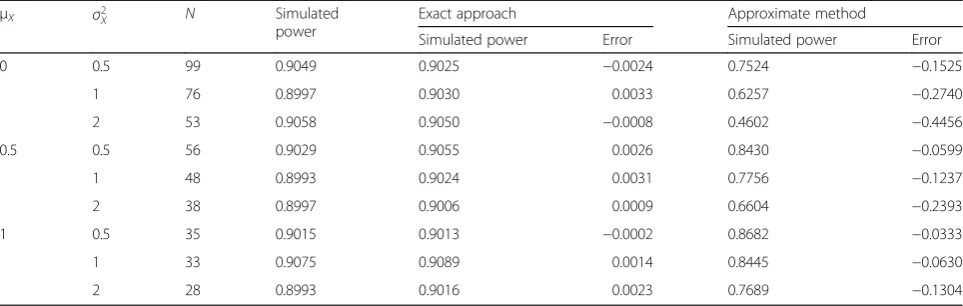
Throughout this empirical investigation, the signifi-cance level and nominal power are fixed asα= 0.05 and 1 –β= 0.90, respectively. With the prescribed specifica-tions, the required sample sizes are computed for the exact procedure with the power function ΨJ. The com-puted sample sizes of the nine combined predictor mean and variance patterns are summarized in Table 2, Table S1 and Table S2 for the coefficient differenced= 0.3, 0.4, and 0.5, respectively. As suggested by a referee, Tables S1 and S2 are presented in Additional files 3 and4, re-spectively. In order to evaluate the accuracy of power calculations, the estimated power of the exact and ap-proximate procedures are also presented. Note that the attained values of the exact approach are marginally lar-ger than the nominal level 0.90. In contrast, the esti-mated powers of the approximation of Colosimo et al. [22] are all less than 0.90 and the difference is quite
Table 1Computed sample size, estimated power, and difference for the exact and approximate procedures with {βI,βS} = {4.1, 0.15}, {βI0,βS0} = {4.198, 0.143},σ2= 0.095,μX= 24.2,σ2X= 6, and Type I errorα= 0.05
Nominal power
Exact approach Approximate method Difference
N Estimated power N Estimated power N Power
0.80 173 0.8001 183 0.8236 10 0.0235
substantial in some cases. Then, Monte Carlo simulation studies of 10,000 iterations were performed to compute the simulated power for the designated sample sizes and parameter configurations. For each replicate,Npredictor values were generated from the designated normal distri-bution N(μX, σ2X). The resulting values of normal pre-dictor, intercept and slope coefficients {βI,βS}, and error variance σ2, in turn, determine the configurations for producing N normal outcomes of the simple linear re-gression model defined in Eq. 1. Next, the test statistic
FJ was computed and the simulated power was the pro-portion of the 10,000 replicates whose test statistics FJ exceed the corresponding critical valueF2,ν, 0.05. The ad-equacy of the two sample size procedures is determined by the error between the estimate power and the simu-lated power. The simusimu-lated power and error are also summarized in Table 2, Table S1 and Table S2 for all twenty-seven design schemes.
It can be seen from these results that the discrepancy between the estimated power and the simulated power is considerably small for the proposed exact technique for all model configurations considered here. Specifically, the resulting errors of the 27 designs are all within the small range of −0.0087 to 0.0056. On the other hand, the estimated powers of the approximate method are constantly smaller than the simulated powers. The out-comes show a clear pattern that absolute error decreases with coefficient differencedand predictor meanμX, and increases with predictor variance σ2
X, when all other
configurations are held constant. Notably, the associated absolute errors can be as large as 0.4456, 0.4295, and 0.4183 when μX= 0 and σ2X = 2 ford= 0.3, 0.4, and 0.5
in Table 2, Table S1, Table S2, respectively. It should be noted that most of the sample sizes reported in the em-pirical examination of Colosimo et al. [22] (Table 1) are rather large and impractical. This may explain why the performance of the approximate formula was acceptable in their study. In fact, some of their cases with smaller
sample sizes also showed the same phenomenon that the simple method leads to an underestimate of power level and an overestimated sample size required to achieve the nominal power. Essentially, the simplicity of the approximate formula does come with a huge price in terms of inaccurate power and sample size calculations.
Non-normal predictors
To address the sensitivity issues of the two techniques, power and sample size calculations were also conducted for the regression models with non-normal predictors. For illustration, the model settings in Table 2 with {βID,
βSD} = {0.3, 0.3} are modified by assuming the predictors have four different sets of distributions: Exponential(1), Gamma(2, 1), Laplace(1), and Uniform(0, 1). For ease of comparison, the designated distributions were linearly transformed to have mean μX and variance σ2X as
re-ported in the previous study. Hence, the computed sam-ple sizes associated with the exact procedure and estimated powers of the two methods remain identical for the four non-normal distributions. The simulated powers were obtained with the Monte Carlo simulation studies of 10,000 iterations under the selected model configurations and non-normal predictor distributions. Similar to the numerical assessments in the preceding study, the computed sample sizes, simulated powers, estimated powers, and associated errors of the two competing procedures are presented in Tables S3-S6 of Additional files 5, 6, 7, 8 for the four types of non-normal predictors, respectively.
Regarding the robustness properties of the two procedures, the results in suggest that the performance of the exact approach is slightly affected by the non-normal covariate settings. The high skewness and kurtosis of the Exponential distribution apparently has a more prominent impact on the normal-based power function than the other three cases of Gamma, Laplace, and Uniform distributions. Note that the approximate
Table 2Computed sample size, estimated power, and simulated power for Normal predictors with {βI,βS} = {0.3, 1.3}, {βI0,βS0} = {0,
1},σ2= 1, Type I errorα= 0.05, and nominal power 1–β= 0.90
μX σ2X N Simulated
power
Exact approach Approximate method
Simulated power Error Simulated power Error
0 0.5 99 0.9049 0.9025 −0.0024 0.7524 −0.1525
1 76 0.8997 0.9030 0.0033 0.6257 −0.2740
2 53 0.9058 0.9050 −0.0008 0.4602 −0.4456
0.5 0.5 56 0.9029 0.9055 0.0026 0.8430 −0.0599
1 48 0.8993 0.9024 0.0031 0.7756 −0.1237
2 38 0.8997 0.9006 0.0009 0.6604 −0.2393
1 0.5 35 0.9015 0.9013 −0.0002 0.8682 −0.0333
1 33 0.9075 0.9089 0.0014 0.8445 −0.0630
method only depends on the mean values of the predic-tors and is presumably less sensitive to the variation of predictor distributions. However, the accuracy margin-ally improved in some cases, but genermargin-ally maintains al-most the same performance as in the normal setting presented in Table2. In short, the sensitivity and robust-ness of the suggested exact technique depends on the level of how badly predictor distributions depart from normality structure. On the other hand, the performance assessments show that the exact procedure still give ac-ceptable results even in the situations with non-normal predictors considered here. More importantly, these em-pirical evidences reveal that the exact approach is rela-tively more reliable and accurate than the approximate method to be recommended as a trustworthy technique for power and sample calculations.
Discussion
In practice, a research study requires adequate statistical power and sufficient sample size to detect scientifically credible effects. Although multiple linear regression is a well-recognized statistical tool, the corresponding power and sample size problem for model validation has not been adequately examined in the literature. To enhance the usefulness of the joint test of intercept and slope coefficients in linear regression analysis, this article pre-sents theoretical discussions and computational algo-rithms for power and sample size calculations under the random modeling framework. The stochastic nature of predictor variables is taken into account by assuming that they have an independent and identical normal dis-tribution. In contrast, the existing method of Colosimo et al. [22] adopted a direct replacement of mean values for the predictor variables. Consequently, the proposed exact approach has the prominent advantage of accommodating the complete distributional features of normal predictors whereas the simple approximation of Colosimo et al. [22] only includes the mean parameters of the predictor variables.
Conclusions
The presented analytic derivations and empirical results indicate that the approximate formula of Colosimo et al. [22] generally does not give accurate power and sample size calculations. According to the overall accuracy and ro-bustness, the exact approach clearly outperforms the ap-proximate methods as a useful tool in planning validation study. Although the numerical illustration only involves a predictor variable, it embodies the underlying principle and critical feature of linear regression that can be useful in conducting similar evaluations for the more general framework of multiple linear regression.
Additional files
Additional file 1:SAS/IML program for computing the power for the joint test of intercept and slope coefficients. (PDF 60 kb)
Additional file 2:SAS/IML program for computing the sample size for the joint test of intercept and slope coefficients. (PDF 60 kb)
Additional file 3:Table S1.Computed sample size, estimated power, and simulated power for Normal predictors with {βI,βS} = {0.4, 1.4}, {βI0,
βS0} = {0, 1},σ2= 1, Type I errorα= 0.05, and nominal power 1–β= 0.90. (PDF 95 kb)
Additional file 4:Table S2.Computed sample size, estimated power, and simulated power for Normal predictors with {βI,βS} = {0.5, 1.5}, {βI0,
βS0} = {0, 1},σ2= 1, Type I errorα= 0.05, and nominal power 1–β= 0.90. (PDF 96 kb)
Additional file 5:Table S3.Computed sample size, estimated power, and simulated power for transformed Exponential predictors with {βI,βS} = {0.3, 1.3}, {βI0,βS0} = {0, 1},σ2= 1, Type I errorα= 0.05, and nominal power 1–β= 0.90. (PDF 95 kb)
Additional file 6:Table S4.Computed sample size, estimated power, and simulated power for transformed Gamma predictors with {βI,βS} = {0.3, 1.3}, {βI0,βS0} = {0, 1},σ2= 1, Type I errorα= 0.05, and nominal power 1–β= 0.90. (PDF 95 kb)
Additional file 7:Table S5.Computed sample size, estimated power, and simulated power for transformed Laplace predictors with {βI,βS} = {0.3, 1.3}, {βI0,βS0} = {0, 1},σ2= 1, Type I errorα= 0.05, and nominal power 1–β= 0.90. (PDF 95 kb)
Additional file 8:Table S6.Computed sample size, estimated power, and simulated power for transformed Uniform predictors with {βI,βS} = {0.3, 1.3}, {βI0,βS0} = {0, 1},σ2= 1, Type I errorα= 0.05, and nominal power 1–β= 0.90. (PDF 96 kb)
Abbreviations
ANCOVA:Analysis of covariance; ANOVA: Analysis of variance
Acknowledgements
The authors would like to thank the editor and two reviewers for their constructive comments that led to an improved article.
Funding No funding.
Availability of data and materials
The summary statistics are available from the following article: [6].
Authors’contributions
SLJ conceived of the study, and participated in the development of theory and helped to draft the manuscript. GS carried out the numerical computations, participated in the empirical analysis and drafted the manuscript. Both authors read and approved the final manuscript.
Authors’information
SLJ is a professor of Applied Mathematics, Chung Yuan Christian University, Taoyuan, Taiwan 32023. GS is a professor of Management Science, National Chiao Tung University, Hsinchu, Taiwan 30010.
Ethics approval and consent to participate Not applicable.
Consent for publication Not applicable.
Competing interests
The authors declare that they have no competing interests.
Publisher’s Note
Author details
1Department of Applied Mathematics, Chung Yuan Christian University,
Taoyuan, Taiwan 32023, Republic of China.2Department of Management
Science, National Chiao Tung University, Hsinchu, Taiwan 30010, Republic of China.
Received: 31 August 2018 Accepted: 26 February 2019
References
1. Cohen J, Cohen P, West SG, Aiken LS. Applied multiple regression/correlation analysis for the behavioral sciences. 3rd ed. Mahwah: Erlbaum; 2003. 2. Kutner MH, Nachtsheim CJ, Neter J, Li W. Applied linear statistical models.
5th ed. New York: McGraw Hill; 2005.
3. Montgomery DC, Peck EA, Vining GG. Introduction to linear regression analysis. 5th ed. Hoboken: Wiley; 2012.
4. Snee RD. Validation of regression models: methods and examples. Technometrics. 1977;19:415–28.
5. Maddahi J, Crues J, Berman DS, et al. Noninvasive quantification of left ventricular myocardial mass by gated proton nuclear magnetic resonance imaging. J Am Coll Cardiol. 1987;10:682–92.
6. Rose BI, McCallum WD. A simplified method for estimating fetal weight using ultrasound measurements. Obstet Gynecol. 1987;69:671–4. 7. Cohen J. Statistical power analysis for the behavioral sciences. 2nd ed.
Hillsdale: Erlbaum; 1988.
8. Kraemer HC, Blasey C. How many subjects?: Statistical power analysis in research. 2nd ed. Los Angeles: Sage; 2015.
9. Murphy KR, Myors B, Wolach A. Statistical power analysis: a simple and general model for traditional and modern hypothesis tests. 4th ed. New York: Routledge; 2014.
10. Ryan TP. Sample size determination and power. Hoboken: Wiley; 2013. 11. Gatsonis C, Sampson AR. Multiple correlation: exact power and sample size
calculations. Psychol Bull. 1989;106:516–24.
12. Mendoza JL, Stafford KL. Confidence interval, power calculation, and sample size estimation for the squared multiple correlation coefficient under the fixed and random regression models: a computer program and useful standard tables. Educ Psychol Meas. 2001;61:650–67.
13. Sampson AR. A tale of two regressions. J Am Stat Assoc. 1974;69:682–9. 14. Shieh G. Exact interval estimation, power calculation and sample size
determination in normal correlation analysis. Psychometrika. 2006;71:529–40. 15. Shieh G. A unified approach to power calculation and sample size
determination for random regression models. Psychometrika. 2007;72: 347–60.
16. Shieh G. Exact analysis of squared cross-validity coefficient in predictive regression models. Multivar Behav Res. 2009;44:82–105.
17. Kelley K. Sample size planning for the squared multiple correlation coefficient: accuracy in parameter estimation via narrow confidence intervals. Multivar Behav Res. 2008;43:524–55.
18. Krishnamoorthy K, Xia Y. Sample size calculation for estimating or testing a nonzero squared multiple correlation coefficient. Multivar Behav Res. 2008; 43:382–410.
19. Shieh G. Sample size requirements for interval estimation of the strength of association effect sizes in multiple regression analysis. Psicothema. 2013;25:402–7. 20. Shieh G. Power and sample size calculations for contrast analysis in
ANCOVA. Multivar Behav Res. 2017;52:1–11.
21. Tang Y. Exact and approximate power and sample size calculations for analysis of covariance in randomized clinical trials with or without stratification. Stat Biopharm Res. 2018;10:274–86.
22. Colosimo EA, Cruz FR, Miranda JLO, et al. Sample size calculation for method validation using linear regression. J Stat Comput Simul. 2007;77:505–16. 23. Binkley JK, Abbot PC. The fixedXassumption in econometrics: can the
textbooks be trusted? Am Stat. 1987;41:206–14.
24. Cramer EM, Appelbaum MI. The validity of polynomial regression in the random regression model. Rev Educ Res. 1978;48:511–5.
25. Shaffer JP. The Gauss-Markov theorem and random regressors. Am Stat. 1991;45:269–73.
26. Rencher AC, Schaalje GB. Linear models in statistics. 2nd ed. Hoboken: Wiley; 2007.