R E S E A R C H A R T I C L E
Open Access
Comparing performance between
log-binomial and robust Poisson regression
models for estimating risk ratios under
model misspecification
Wansu Chen
1*, Lei Qian
1, Jiaxiao Shi
1and Meredith Franklin
2Abstract
Background:Log-binomial and robust (modified) Poisson regression models are popular approaches to estimate risk ratios for binary response variables. Previous studies have shown that comparatively they produce similar point estimates and standard errors. However, their performance under model misspecification is poorly understood.
Methods:In this simulation study, the statistical performance of the two models was compared when the log link function was misspecified or the response depended on predictors through a non-linear relationship (i.e. truncated response).
Results:Point estimates from log-binomial models were biased when the link function was misspecified or when the probability distribution of the response variable was truncated at the right tail. The percentage of truncated observations was positively associated with the presence of bias, and the bias was larger if the observations came from a population with a lower response rate given that the other parameters being examined were fixed. In contrast, point estimates from the robust Poisson models were unbiased.
Conclusion:Under model misspecification, the robust Poisson model was generally preferable because it provided unbiased estimates of risk ratios.
Keywords:Log-binomial regression, Robust (modified) Poisson regression, Model misspecification, Risk ratio, Link function misspecification
Background
Introduction
Logistic regression is the most widely-used modeling ap-proach for studying associations between exposures and binary outcomes. For rare events, the odds ratio estimated from logistic regression approximates the risk ratio (RR). However, when events are common, odds ratios always overestimate risk ratios [1] Zhang and Yu [2] suggested a correction for odds ratios to give a risk ratio in studies of common outcomes. This method was subsequently shown to result in inconsistent point estimates as well as invalid confidence intervals [3]. Efforts were made to modify the data so that estimated odds ratios from a logistic
regression analysis were comparable to risk ratios [4]. However, it was found that these methods produced prevalence greater than one [5]. Greenland [6] brought ex-tensive literature on valid model-based estimation of rela-tive risks and other measures to readers’attention. Of the model-based approaches, log-binomial [5,7,8] and robust (or modified) Poisson regression models [7, 9] are most frequently applied to estimate risk ratios for common bin-ary outcomes. Barros et al. [7] and Zou [9] showed how risk ratios can be estimated by using robust Poisson re-gression with a robust error variance.
In medical and public health research, log-binomial and robust Poisson regression models are widely used to directly estimate risk ratios for both common and rare outcomes. For example, they can be used to estimate the effect of clinical characteristics (e.g. obesity, smoking, history of stroke, exercise, or diet) on a health condition * Correspondence:[email protected]
1Kaiser Permanente Southern California, Department of Research and Evaluation, 100 S. Los Robles Ave, 2nd Floor, Pasadena, CA 91101, USA Full list of author information is available at the end of the article
(e.g. a cardiovascular event, mortality, or hospital admis-sion). Our own Medline search of articles published be-tween 2005 and 2014 demonstrated that the popularity of both models has increased significantly in the past decade (Additional file1).
Model misspecification can lead to biased estimates, resulting in erroneous and misleading conclusions. Re-gression models require that the relationship between the response and the explanatory variables conforms to a particular functional form. Omitting important ex-planatory variables, failing to account for non-linear components or critical interaction terms, or making measurement errors can cause model misspecification and thus bias the parameter estimators of one or more of the predictors in a regression model. Under correct model specification, the log-binomial and robust Poisson methods have been shown to yield comparable point es-timates and standard errors [7,9–12]. For instance, in a simulation study with sample size of 1000, both the log-binomial and robust Poisson models yielded similar unbiased estimates with good coverage probability [12]. However, the results of the following example revealed a different paradigm.
A motivating example
A cross-sectional study was conducted at Kaiser Perma-nente Southern California to assess the association of fractional exhaled nitric oxide (FeNO), a marker of air-way inflammation, and asthma burden among persistent asthma patients who were treated with inhaled cortico-steroids (ICS). It was hypothesized that high FeNO levels were associated with greater asthma burden. In this study, the primary binary outcome of interest was whether seven or more short-acting beta-agonist (SABA) canisters were dispensed in the past 12 months, which is a validated administrative data surrogate for asthma im-pairment. Previous studies based on similar patient pop-ulations revealed that the prevalence of asthma impairment among persistent asthma patients was high [13]. The study population consisted of asthma patients 12 to 56 years of age who had aeroallergen sensitization and regular ICS treatment for at least one month were enrolled during an allergy department visit (index visit). Information on patient demographics, FeNO, forced ex-piratory volume in one second (FEV1% predicted) and
asthma control test (ACT) score was collected during the index visit, while the information on aeroallergen sensitization and SABA canisters dispensed came from electronic medical records.
FeNO was categorized into four quartiles. Multivari-able log-binomial and robust Poisson regression models were applied to estimate the risk ratio of having seven or more SABA canisters in each of the FeNO quartiles (using the lowest quartile as the reference group),
controlling for age, gender, race/ethnicity, number of aeroallergen sensitivities, clinical center, FEV1%
pre-dicted (≥80% vs. < 80%) and ACT score (> 19, 16–19, < 16). Age remained as a continuous variable in the model.
Based on the robust Poisson model, the risk ratio of having ≥7 SABA canisters over the past 12 months was 2.05 (95% CI, 1.03–4.05) in patients whose FeNO value was in the second quartile, compared to patients whose FeNO value was in the first quartile (Additional file 2). However, when the analysis was repeated by using the log-binomial model, the corresponding risk ratio was 1.67 (95% CI, 0.83–3.57), a 19% reduction from the ro-bust Poisson estimate. Although the point estimates for FeNO from the two models were in the same direction, the interpretation of the results varied because the 95% confidence interval of the estimated RR from the robust Poisson covered one, yet the log-binomial model did not. The RR for patients whose FeNO values were in the third and fourth quartiles compared to the patients in the first quartile were also different between the two models, although the interpretations remained the same at the 95% level (see Additional file 2). The differences in point estimates of RR between the two models were in the range of 12–19%.
Current study
The inconsistent conclusions between the aforemen-tioned simulation studies [7,9–12] and the results from the motivating example led us to further investigate whether model misspecification and/or characteristics of the data resulted in such large discrepancies between log-binomial and the robust Poisson regression models.
The paper is organized as follows: The “Methods” section presents the theory behind the two models to explain the differences in the estimation methods that could result in variations in the estimates. The "Methods" section also provides the details of the simulation design. The "Results" section shows the results of simulation under various scenarios. Lastly, we summarize the find-ings and provide recommendations for the use of these models in future studies in the“Discussion”section.
Methods
Generalized linear models (GLM) originate from a signifi-cant extension of traditional linear regression models [14]. They consist of a random component that specifies the conditional distribution of the response variable (Y) from an exponential family given the values of the explanatory variablesX1,X2,···,Xk, a linear predictor (or systematic)
com-ponent that is a linear function of the predictors, ƞ=β0+β1X1+β2X2+···+βkXk, where β=(β0,β1,...,βk)T is the vector of the parameters, and a smooth invertible link function that transforms the expectation of the re-sponse variable, μ ≡ E(Y), to the linear predictors:
g(μ)=ƞ=β0+β1X1+β2X2+···βkXk. For example, the most common link for binary outcomes is the logit (i.e. log (μ/(1-μ))) in a logistic model, the log (μ) in a Poisson model, or a log-binomial model.
In the descriptions below,YiandxTi ¼ ð1;xi1;xi2;…;xikÞ denote the binary outcome and the row vector comprised of
k predictors for the ith individual (i = 1,2,…n), respectively. The observations from thenindividuals are independent.
Log-binomial regression
In the GLM framework, the conditional distribution of Yi given the predictor variables is binomial, with the mean re-sponse related to the predictors by the link function log (μi). In log-binomial regression,μiis often denoted aspi, be-cause E(Yi) is a probability with a value between zero and one. Although there are other methods to obtain efficient estimators, the maximum likelihood approach is used to generate asymptotically efficient estimators (maximum like-lihood estimates (MLE)) in log-binomial regressions [5,8].
The MLE of log-binomial models are derived from an iteratively reweighted least squares (IRLS) approach [15]. In a log-binomial regression, logðPiðβÞÞ ¼xTi β where
pi(β)=Pr(yi=1|xi),0 ≤ pi ≤ 1, and xXi β<0 (constrained). The log-likelihood is given by
84%ℓð Þ ¼β X n
i¼1
yi logðpið ÞβÞ þ Xn
i¼1
1−yi
ð Þlog 1ð −pið ÞβÞ
ð1Þ
It can be proven that the MLE forβcan be found by the following iteration (Additional file4)
βðtþ1Þ¼ðX0WXÞ−1 X0 Wz
ð2Þ
where z¼XβðtÞþ Y−P β
t ð Þ
Pβð Þt ;X¼ xi;j ∈R n;k;
Y−Pð Þβ
Pð Þβ ¼
y1−p1ð Þβ p1ð Þβ
;y2−p2ð Þβ p2ð Þβ
;…;yn−pnð Þβ
pnð Þβ
T
;
and weight W¼Diag pið Þβ 1−pið Þβ
;
i¼1;2;…;n;j¼1;2;…;k:
The iteration process continues until βstabilizes. The weights W used in the iterative process contain pi(β) in the numerator and 1 –pi(β) in the denominator, where
pi(β) = exp (xTi β) with a range from 0 to 1. Whenpi(β) is a very small number, the weight approximates pi(β). When pi(β) approaches one, the weight approaches in-finity. This suggested that the IRLS approach is highly influenced by observations that have large pi(β). More-over, the impact is also influenced by the average pi(β), or the average weight (lower average pi(β) is associated with lower average weight). For illustration, we con-structed two hypothetical samples each with five obser-vations having the following probabilities: sample 1 = {0.1, 0.3, 0.4, 0.5, 0.95} and sample 2 = {0.02, 0.03, 0.08, 0.15, 0.95}. The corresponding weights for the two sam-ples were {0.25, 0.43, 0.67, 1, 19} and {0.02, 0.03, 0.09, 0.18, 19}, respectively. In sample 2, the observation with weight 19 will impact the point estimate more, com-pared the observation in sample 1 with the same weight.
Robust Poisson regression
In robust Poisson regression, a quasi-likelihood (QL) model can be applied to fit the data with a binary out-come [14–18]. Quasi-likelihood was first introduced by Wedderburn (1974) as a function that has properties analog to those of log-likelihood functions [18]. Similar to ML method, maximum QL method can be used to es-timate the QL eses-timates. In a maximum QL model, only the relationship between the mean and the variance (i.e. the variance is a function of the mean) needs to be spe-cified instead of the underlying distribution of the data [15–19]. It can be shown that when Yi comes from the exponential family, the quasi-score function is identical to the score function associated with the maximum like-lihood of the GLM.
When the Poisson distribution is chosen, the quasi-score function can be simplified toSjðβÞ ¼ϕ1Pni¼1 ðyi−μiÞxij, resulting in quasi-score estimating equations
and j = 1,2,…k. The final estimate from the quasi-scoring procedure satisfies the conditionSjðβ^Þ ¼0 and ^β is a consistent and asymptotically unbiased esti-mate ofβ[20].^βdoes not depend onϕ.
The quasi-likelihood estimators are not maximally and asymptotically efficient [14]. The robust Poisson regres-sion model uses the classical sandwich estimator under the generalized estimation equation (GEE) framework to provide accurate standard errors for the elements [19–21]. The variance-covariance matrix is
Xn
i¼1 E I½ið Þβ
" #−1 Xn
i¼1
E ðSið ÞβSið ÞβT
h i
" #−1 Xn
i¼1 E I½ið Þβ
" #−1
ð3Þ
where IiðβÞ ¼−∂S∂iðβÞβ is the information matrix [22]. A consistent estimate of the variance can be obtained by evaluating the variance-covariance matrix at^β.
Implementation
Both regression models were implemented in SAS [23]
(SAS Software Version 9.3 of the SAS System for Unix.
Cary, NC. SAS Institute Inc. 2011). The SAS codes can be found in Additional file5. For the log-binomial model,−4 was set as the initial value of the intercept. For both models, the weighted least squares estimates (default) were used as initial values of parameters. The convergence criterion was 10−4 (default). A well-known issue of log-binomial models is failure to converge when the MLE is located on the boundary of the parameter space (i.e. the predicted probability of the outcome is equal to 1). To minimize the convergence issue, the COPY method was applied [24,25] in which the number of virtual copies was set to 10,000. To ensure a fair comparison between the log-binomial and robust Poisson models, the evaluation was conducted by only using the results based on exactly the same simulated data. If the COPY method did not converge for a dataset, the same dataset was then removed before the performance of the robust Poison models was evaluated. The exclusion of datasets was very rare in this study. Details on the number of excluded datasets can be found in the“Discussion”section.
Measures of model performance
For each simulated scenario, the simulation process was repeated 1000 times. In each of the 1000 simulated data-sets, the log risk ratio was estimated from the log-binomial model and the robust Poisson model, re-spectively. For each scenario, the relative bias, standard error (SE), and mean square error (MSE) in log scale for all three measures were calculated by summarizing the results from the 1000 datasets for each regression model.
Relative bias was defined as the average of the 1000 esti-mated RR in log scale minus the log of the true RR divided by the log of the trueRR. For θ^m, the estimated log RR from the mth dataset using either the log-binomial model or the robust Poisson model, the
rela-tive bias was defined as
1 1;000
P
m¼1 1;000 ^θ
m−logðtrueRRÞ logðtrueRRÞ
100%. Standard error was defined as the empirical SE of the esti-mated risk ratio in log scale over all 1000 simulations. The MSE was calculated by taking the sum of the squared bias in log scale and the variances, in which the bias was
speci-fied as 1 1;000
P
m¼1 1;000
^
θm−logðtrueRRÞ.
Because both SE and MSE depended on the sample size, the process described above was repeated for sam-ple of size 500 for all scenarios with RR = 3.
Simulated datasets
Let Y be a common binary outcome (Y= 1 for disease and Y= 0 for non-disease) and X be a binary exposure variable (X= 1 for exposure andX= 0 for non-exposure). First, uncorrelated random variablesZ1andZ2following
the Bernoulli (0.5) and the Uniform [0, 1] distributions, respectively, were generated for 1000 subjects. These distributions were chosen for their simplicity in the de-sign. Then, the exposure variable X based on the subject-specific probability of exposure, defined by the equation logit (P (X= 1| Z1, Z2)) =−1.0 +Z1+Z2 with
E(P(X= 1| Z1, Z2)) = 0.5, was created for each subject.
All of the outcome variables defined below were condi-tional on the exposure status and the covariates. For exposed subjects, P (Y= 1| X= 1, Z1, Z2) = 3 ×P (Y= 1| X= 0, Z1, Z2). The adjusted RR (i.e. P (Y= 1| X= 1, Z1, Z2)) /P (Y= 1|X= 0,Z1,Z2)) was fixed at 3.0, chosen to
reflect the effect size commonly seen in real-world set-tings, and strong enough to yield observable differences in performance between the two regression models.
Scenarios to study the impact of truncation
The equations to generateYtook four different forms (Y1,
Y2,Y3,Y4) to enable the examination of the impact of
trun-cation. UnlikeY1, which always had a perfect linear
associ-ation with its predictors (i.e. not truncated),Y2,Y3,andY4
were truncated such that the values ofP(Yk= 1|X= 0,Z1, Z2) depended on whether or not“Z1+ (beta of Z2) ×Z2”
reached a threshold (k= 2, 3, and 4) (Table 1). For ex-ample, in Scenario I-2, the threshold was set at 0.15, requiring“Z1+ 3 ×Z2”to be greater than 0.15 to impact P(Y2= 1|X= 0,Z1,Z2)). The defined threshold varied by
scenario and was chosen such that the percentages of ex-posed subjects at the maximumP(Y= 1|X,Z1,Z2)) could
X, Z1, Z2)) for both exposed and unexposed subjects.
When other parameters were fixed, a spike goes higher with the increase of the threshold. This allowed us to study how the volume of large P (Y= 1| X, Z1, Z2))
im-pacted model performance.
Scenarios to study the impact of maximum P(Y = 1)
First, scenarios I-1, II-1, and III-1 were created using the log link function. The maximum values ofP(Y1= 1|X= 1, Z1, Z2)) were set to 0.75, 0.85 and 0.95, respectively,
to study the impact of maximum P (Y1= 1| X= 1, Z1, Z2)) (Table 1). The selected thresholds were set at 0.15,
0.30, and 0.60 for Y2,Y3, and Y4, respectively. The
per-centages of exposed subjects who were at the maximum
values set above (0.75, 0.85, and 0.95) were 1.4, 2.8, and 5.8%. These values were derived by simulation and rep-resented the various levels of alteration of the linear predictors.
The intercepts were manually calculated to satisfy P (Yk= 1 | X= 0, Z1, Z2)≤0.75/3, 0.85/3 and 0.95/3,
re-spectively. For example, for the equation log (P (Y1= 1| X= 0, Z1, Z2)) =α – Z1–3 *Z2 in scenario I-1, α=
log(0.75/3) =−1.38 since the logarithm is an increasing function and hence the maximum ofP(Y1= 1|X= 0,Z1, Z2) is achieved when Z1 = 0 and Z2= 0. For the same
reason, for the equation log (P(Y2= 1|X= 0,Z1,Z2)) =α
– Z1 – max (Z1+ 3 *Z2, 0.15) in scenario I-2, α=
log(0.75/3) + 0.15 =−1.23. The 12 scenarios designed to
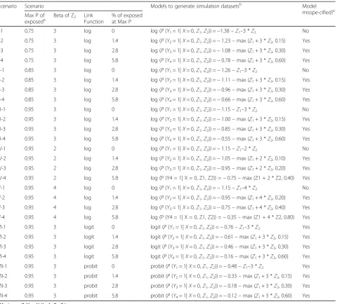
Table 1Design of the simulation data
Scenario Scenario Models to generate simulation datasetsb Model
misspe-cified?c Max P of
exposeda Beta of Z2 LinkFunction % of exposedat Max P
I-1 0.75 3 log 0 log (P(Y1= 1|X= 0,Z1,Z2)) =−1.38–Z1–3 *Z2 No
I-2 0.75 3 log 1.4 log (P(Y2= 1|X= 0,Z1,Z2)) =−1.23–max (Z1+ 3 *Z2, 0.15) Yes
I-3 0.75 3 log 2.8 log (P(Y3= 1|X= 0,Z1,Z2)) =−1.08–max (Z1+ 3 *Z2, 0.30) Yes
I-4 0.75 3 log 5.8 log (P(Y4= 1|X= 0,Z1,Z2)) =−0.78–max (Z1+ 3 *Z2, 0.60) Yes
II-1 0.85 3 log 0 log (P(Y1= 1|X= 0,Z1,Z2)) =−1.26–Z1–3 *Z2 No
II-2 0.85 3 log 1.4 log (P(Y2= 1|X= 0,Z1,Z2)) =−1.11–max (Z1+ 3 *Z2, 0.15) Yes
II-3 0.85 3 log 2.8 log (P(Y3= 1|X= 0,Z1,Z2)) =−0.96–max (Z1+ 3 *Z2, 0.30) Yes
II-4 0.85 3 log 5.8 log (P(Y4= 1|X= 0,Z1,Z2)) =−0.66–max (Z1+ 3 *Z2, 0.60) Yes
III-1 0.95 3 log 0 log (P(Y1= 1|X= 0,Z1,Z2)) =−1.15–Z1–3 *Z2 No
III-2 0.95 3 log 1.4 log (P(Y2= 1|X= 0,Z1,Z2)) =−1.00–max (Z1+ 3 *Z2, 0.15) Yes
III-3 0.95 3 log 2.8 log (P(Y3= 1|X= 0,Z1,Z2)) =−0.85–max (Z1+ 3 *Z2, 0.30) Yes
III-4 0.95 3 log 5.8 log (P(Y4= 1|X= 0,Z1,Z2)) =−0.55–max (Z1+ 3 *Z2, 0.60) Yes
IV-1 0.95 2 log 0 log (P(Y1= 1|X= 0,Z1,Z2)) =−1.15–Z1–2 *Z2 No
IV-2 0.95 2 log 1.4 log (P(Y2= 1|X= 0,Z1,Z2)) =−1.05–max (Z1+ 2 *Z2, 0.10) Yes
IV-3 0.95 2 log 2.8 log (P(Y3= 1|X= 0,Z1,Z2)) =−0.95–max (Z1+ 2 *Z2, 0.20) Yes
IV-4 0.95 2 log 5.8 log (P (Y4 = 1| X = 0, Z1, Z2)) =−0.75–max (Z1 + 2 * Z2, 0.40) Yes
V-1 0.95 4 log 0 log (P(Y1= 1|X= 0,Z1,Z2)) =−1.15–Z1–4 *Z2 No
V-2 0.95 4 log 1.4 log (P(Y2= 1|X= 0,Z1,Z2)) =−0.95–max (Z1+ 4 *Z2, 0.20) Yes
V-3 0.95 4 log 2.8 log (P(Y3= 1|X= 0,Z1,Z2)) =−0.75–max (Z1+ 4 *Z2, 0.40) Yes
V-4 0.95 4 log 5.8 log (P (Y4 = 1| X = 0, Z1, Z2)) =−0.35–max (Z1 + 4 * Z2, 0.80) Yes
VI-1 0.95 3 logit 0 logit (P(Y1= 1|X= 0,Z1,Z2)) =−0.76–Z1–3 *Z2 Yes
VI-2 0.95 3 logit 1.4 logit (P(Y2= 1|X= 0,Z1,Z2)) =−0.61–max (Z1+ 3 *Z2, 0.15) Yes
VI-3 0.95 3 logit 2.8 logit (P(Y3= 1|X= 0,Z1,Z2)) =−0.46–max (Z1+ 3 *Z2, 0.30) Yes
VI-4 0.95 3 logit 5.8 logit (P(Y4= 1|X= 0,Z1,Z2)) =−0.16–max (Z1+ 3 *Z2, 0.60) Yes
VII-1 0.95 3 probit 0 probit (P(Y1= 1|X= 0,Z1,Z2)) =−0.48–Z1–3 *Z2 Yes
VII-2 0.95 3 probit 1.4 probit (P(Y2= 1|X= 0,Z1,Z2)) =−0.33–max (Z1+ 3 *Z2, 0.15) Yes
VII-3 0.95 3 probit 2.8 probit (P(Y3= 1|X= 0,Z1,Z2)) =−0.18–max (Z1+ 3 *Z2, 0.30) Yes
VII-4 0.95 3 probit 5.8 probit (P(Y4= 1|X= 0,Z1,Z2)) =−0.12–max (Z1+ 3 *Z2, 0.60) Yes
a
MaximumP(Yk= 1|X= 1,Z1,Z2) b
Models to generateYkfor unexposed subjects. For exposed subjects,P(Yk= 1|X= 1,Z1,Z2) =3*P(Yk= 1|X= 0,Z1,Z2). k = 1, 2, 3, and 4 c
study the impact of largeP(Y = 1) were listed in the first section of Table1(in the first 12 rows).
Scenarios to study the impact of coefficient of Z2
To study the impact of the entire distribution of
P(Y = 1)when largeP(Y = 1)existed, eight more scenar-ios were produced, with the beta coefficient ofZ2being
2 and 4 (shown in the middle section of Table1), to join the four scenarios for which the beta coefficient of Z2
was set to 3 (i.e. III-1, III-2, III-3, and III-4). The distri-bution ofP(Y = 1) was shifted towards zero as the beta coefficient ofZ2increased. Thus, these scenarios allowed
us to study the impact of the outcome distribution, or the averageP(Y = 1).
The intercepts and the thresholds were generated using the same approach as described in the previous section. BecauseZ2follows the uniform distribution, the
thresholds increase proportionally with the beta coeffi-cients. For example, the threshold to make 1.4% of ex-posed subjects reached the maximum P (Y2= 1| X= 1,
Z1,Z2) = 0.1 when the beta ofZ2was 2 and increased to
0.2 when the beta ofZ2was 4.
Scenarios to study the impact of misspecified link functions
The link function was altered from log to logit and pro-bit in scenarios VI and VII to assess the model perform-ance when the link functions were misspecified; refer to the last section of Table 1. For scenarios VI-2, VI-3, VI-4, VII-2, VII-3, and VII-4, not only were the link functions misspecified, but also the responses depended on covariates with truncated probabilities.
Scenarios with a weaker association between exposure and outcome (RR = 2)
To understand the impact of misspecified link functions and truncation when RR is different from 3.0, we also generated scenarios with parameters identical to those in III-1, III-2, III-3, III-4, VII-1, VII-2, VII-3 and VII-4, ex-cept that this time RR = 2.0 instead of 3.0.
Results
Relative bias
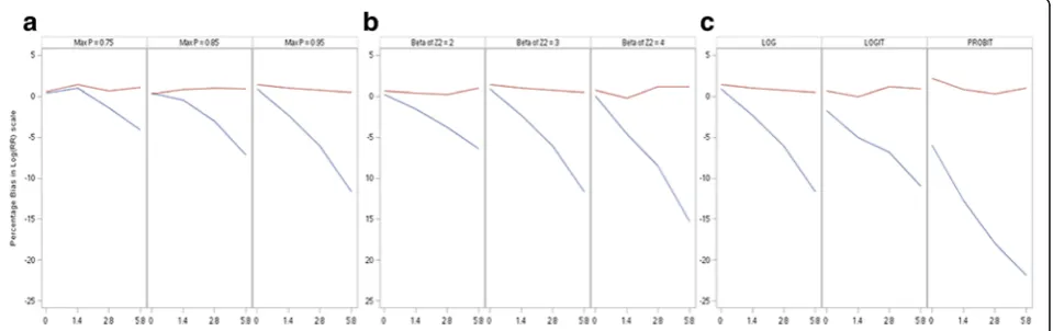
The relative biases of the estimatedRR in log scale from the two models in each of the 28 scenarios when n= 1000 are shown in Table2and Fig.1.
As expected, both models accurately estimatedβ1or log
(RR) when they were correctly specified, regardless of the value of the maximumP. When the models were misspe-cified (as shown in the shaded areas in Table2), the rela-tive biases of the robust Poisson models were negligible, while those of log-binomial models tended to negatively bias away from null. For the log-binomial models, the magnitude of biases increased in all scenarios when the
level of misspecification, measured by the percentage of exposed subjects at maximumP, increased.
Large P(Y = 1) was associated with an increased level of bias when the percentage of exposed subjects having the max P (Yk= 1|X= 1, Z1, Z2) was fixed; refer to the
first three rows of Table 2 and Fig. 1, Panel A. For ex-ample, when the percentage of exposed subjects whose maximum P (Yk= 1| X= 1, Z1, Z2) was fixed at 5.8, an
increase of maximum P(Yk= 1|X= 1,Z1,Z2) from 0.75
(scenario I-4) to 0.95 (scenario III-4) resulted a change in relative bias from−4.1% to−11.7%.
The impact of averageP(Y = 1)was displayed from the 4th to the 6th rows of Table2 and in Panel B of Fig.1. When the percentage of exposed subjects having the maxP (Yk= 1|X= 1,Z1,Z2) was fixed, the log-binomial
models were more vulnerable (larger absolute value of relative biases) when the beta coefficient of Z2increased
(i.e. average P (Y= 1| X= 1, Z1, Z2) decreased). For
ex-ample, when the percentage of exposed subjects whose maximumP(Yk= 1|X= 1,Z1,Z2) = 2.8, the relative bias
changed from−3.8% to−8.5% when the beta coefficient increased from 2 to 4. This indicates that the value of the average P(Y = 1) impacts the performance of the log-binomial models. When there were enough large
P(Y = 1), a low average P(Y = 1) away from large
P(Y = 1)was associated with a large relative bias. When the underlying distribution of data was logit, misspecifying the link function as ‘log’ did not signifi-cantly influence relative biases. However, when the underlying distribution of data was probit, the bias (− 5.9%) was noticeable even when the linear predictors were properly specified (i.e. percentage of exposed sub-jects having the maxP (Yk= 1|X= 1, Z1,Z2) was zero).
Refer to the last three rows of Table 2 and Panel C of Fig.1. Misspecifying the link function from log to probit in the presence of misspecified linear predictors had a serious consequence. The relative bias was almost−18% when the percentage of exposed subjects at the max-imumPwas only 2.8.
Standard error
In all simulation scenarios, the SE of the two models were comparable (Table 3). At the 2nd decimal point, the SE derived from the log-binomial models were either the same or slightly smaller compared to those of robust Poisson models. The largest difference, 0.03 (=0.23– 0.20), occurred when the data distribution was probit, maximumP(Y= 1|X= 1,Z1,Z2) was 0.95, and the beta
of Z2was 3 (scenario VII-1). When the models correctly
the 3rd decimal place, even if the models were correctly specified (data not shown).
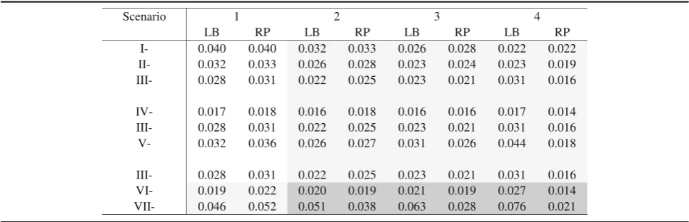
Mean square error
As expected, when the models were correctly specified (in the unshaded area in Table 4), log-binomial models yielded the same or marginally smaller MSE compared to robust Poisson models. When the underlying distribution of data had a log or logit link (scenarios I-VI) and the per-centage of exposed subjects having the maxP(Yk= 1|X= 1,Z1,Z2) was 1.4% or 2.8% (in the columns labeled as‘2’
and‘3’in Table4), the MSE of the two models were still comparable, except for one scenario. The exception oc-curred in scenario V-3, where the superiority of the robust Poisson models was quite noticeable; the difference in MSE between the two models was 0.05. Recall that the averageP(Y = 1)for V-3 was smallest among all three sce-narios (III-3, IV-3 and V-3) and followed by that of III-3. Thus, it is not surprising to observe the difference
between the two models becoming larger from IV-3 to III-3, and to V-3. For scenarios III-4 to VII-4, the robust Poisson models consistently outperformed the log-binomial models. For scenarios of VII (in which the underlying data were generated using a probit link), the MSE of log-binomial models, compared to those of robust Poisson models, were slightly smaller when the linear pre-dictors were properly specified (such as in scenario VII-1) and significantly larger when the linear predictors were improperly specified, even when level of misspecification of the linear predictors was small. For example, when the percentage of exposed subjects at the 0.95 (max P) was only 1.4, the MSE were 0.051 and 0.038, from the log-binomial model and the robust Poisson model, respectively.
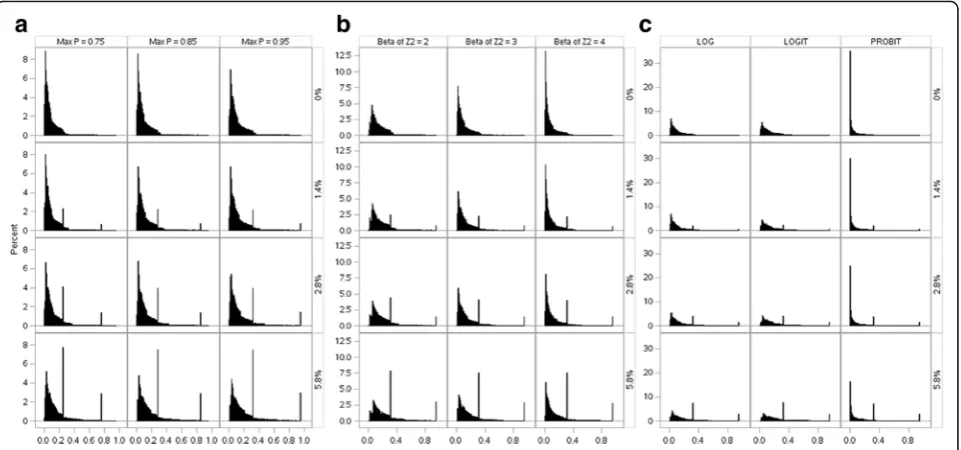
Distribution of P(Y = 1)
The distributions ofP(Y = 1) for all simulated data (one million data points for each scenario) are shown in Fig.2.
Table 2Relative bias (%) in log scale with and without model misspecification (n= 1000)
Scenario 1 2 3 4
LB RP LB RP LB RP LB RP
I- 0.4 0.6 1.0 1.5 -1.4 0.7 -4.1 1.1
II- 0.4 0.3 -0.5 0.8 -3.0 1.0 -7.1 0.9
III- 0.9 1.4 -2.3 1.0 -6.1 0.8 -11.7 0.5
IV- 0.2 0.6 -1.5 0.4 -3.8 0.2 -6.4 1.0
III- 0.9 1.4 -2.3 1.0 -6.1 0.8 -11.7 0.5
V- 0.1 0.7 -4.6 -0.2 -8.5 1.2 -15.4 1.2
III- 0.9 1.4 -2.3 1.0 -6.1 0.8 -11.7 0.5
VI- -1.7 0.6 -5.0 0.0 -6.8 1.2 -11.0 0.9
VII- -5.9 2.2 -12.8 0.9 -18.0 0.4 -21.9 1.0
Unshaded: Models were correctly specified
Light shaded: Misspecified linear predictors or misspecified link function Dark shaded: Misspecified linear predictors and misspecified link function LB: log-binomial, RP: robust Poisson
Change of scenarios: Increasing intercept: I→II→III; Increasing coefficient ofβ2: IV→III→V; Change of link function: III (log), VI (logit), VII (probit)
Fig. 1Percentage bias in log(RR) scale.aFrom left to right: increasing intercept(scenario I→II→III);bFrom left to right: increasing coefficient of
Panel A shows the distribution of P(Y = 1) with varying maximumP(Y = 1). When the link function and beta of
Z2 were fixed at‘log’and 3, respectively, an increase of
maxP(Y = 1)from 0.75 (scenario I) to 0.95 (scenario III) stretched the spikes to the right (Fig.2Panel A).
Panel B shows the distribution with varying beta of Z2.
When the beta ofZ2increased from 2 (scenario VI) to 4
(scenario V) while the maxP(Y = 1)was fixed at 0.95 and the link function was set as‘log,’the distribution ofP(Y = 1) became taller, thinner, and shifted towards zero. This provides the evidence that attributes the increase of biases to the downward shift of the distribution of P(Y = 1)(i.e. decrease in the prevalence of the outcome variableY).
Panel C shows the distribution with varying link func-tion. Spikes (i.e. vertical thin lines in all figures except those labeled with “0% at the max P”) for both exposed
and unexposed subjects increased in all scenarios when the percentage of exposed subjects at the max P(Y = 1) increased from 1.4, 2.8 to 5.8%, indicating a higher level of violation of the linearity assumption. The distribu-tions of P(Y = 1) for data with log and logit link func-tions were similar; however, the distribufunc-tions of P(Y = 1) for data with probit link function distinguished them-selves significantly from those of log or logit. This obser-vation explains the larger biases seen in Fig. 1 Panel C, when the underlying distribution of data were probit, compared to those of log and logit distributions, even when the predictors were perfectly linear.
Results of moderate sample size (n= 500)
When the simulation was conducted based on samples of moderate size (n = 500), the same pattern was observed
Table 3Standard error in log scale with and without model misspecification (n = 1000)
Scenario 1 2 3 4
LB RP LB RP LB RP LB RP
I- 0.20 0.20 0.18 0.18 0.16 0.17 0.14 0.15
II- 0.18 0.18 0.16 0.17 0.15 0.15 0.13 0.14
III- 0.17 0.17 0.15 0.16 0.14 0.15 0.12 0.13
IV- 0.13 0.13 0.13 0.13 0.12 0.13 0.11 0.12
III- 0.17 0.17 0.15 0.16 0.14 0.15 0.12 0.12
V- 0.18 0.19 0.15 0.16 0.15 0.16 0.12 0.13
III- 0.17 0.17 0.15 0.16 0.14 0.15 0.12 0.13
VI- 0.14 0.15 0.13 0.14 0.13 0.14 0.11 0.12
VII- 0.20 0.23 0.18 0.19 0.16 0.17 0.14 0.15
Unshaded: Models were correctly specified
Light shaded: Misspecified linear predictors or misspecified link function Dark shaded: Misspecified linear predictors and misspecified link function LB: log-binomial, RP: robust Poisson
Change of scenarios: Increasing intercept: I→II→III; Increasing coefficient ofβ2: IV→III→V; Change of link function: III (log), VI (logit), VII (probit)
Table 4Mean square error (MSE) in log scale with and without model misspecification (n = 1000)
Scenario 1 2 3 4
LB RP LB RP LB RP LB RP
I- 0.040 0.040 0.032 0.033 0.026 0.028 0.022 0.022
II- 0.032 0.033 0.026 0.028 0.023 0.024 0.023 0.019
III- 0.028 0.031 0.022 0.025 0.023 0.021 0.031 0.016
IV- 0.017 0.018 0.016 0.018 0.016 0.016 0.017 0.014
III- 0.028 0.031 0.022 0.025 0.023 0.021 0.031 0.016
V- 0.032 0.036 0.026 0.027 0.031 0.026 0.044 0.018
III- 0.028 0.031 0.022 0.025 0.023 0.021 0.031 0.016
VI- 0.019 0.022 0.020 0.019 0.021 0.019 0.027 0.014
VII- 0.046 0.052 0.051 0.038 0.063 0.028 0.076 0.021
Unshaded: Models were correctly specified
Light shaded: Misspecified linear predictors or misspecified link function Dark shaded: Misspecified linear predictors and misspecified link function LB: log-binomial, RP: robust Poisson
in terms of relative biases and SE (Additional file6, Tables AF6.1-AF6.2). As expected, the SE based on the samples of moderate size was larger compared to those derived from samples with n= 1000. The same pattern was also observed for MSE (Additional file 6, Table AF6.3); how-ever, the differences between the two models were not as substantial as seen in the samples of sizes 1000.
Results with a weaker association between exposure and outcome (RR = 2)
When the simulation was conducted based on simula-tion datasets with RR = 2, the relative biases were similar to those of the corresponding scenarios with RR = 3 (data not shown). The standard errors derived from the simulation datasets with RR = 2 were 12–36% smaller compared to those of the corresponding scenarios with RR = 3; however, the pattern remained the same. That is, the standard errors of the two models were comparable with those from the robust Poisson models being only slightly larger than those from the log-binomial models. The MSE yielded from the simulation datasets with RR = 2 were 16–47% smaller compared to those of the matching datasets with RR = 3. Nevertheless, similar to the patterns observed for RR = 3, the robust Poisson had lower MSE compared to the log-binomial models, and the differences were more dramatic when a probit link was used (versus a log link) and when the data had a higher percentage of truncation.
Discussion
In this study, the statistical performances of the two most popular model-based approaches used to estimate
RR for common binary outcomes were examined when the link function was misspecified or when the probabil-ity of the response variables was truncated at the right tail. Our findings suggest that point estimates from log-binomial models were biased when the link function was misspecified or when the probability distribution of the response variable was truncated for even a small proportion of observations. For log-binomial models, the percentage of truncated observations was positively asso-ciated with the presence of the bias. The bias was more significant if these observations came from a population in which the response rate was lower, given the other parameters being examined were fixed.
For MLE based methods, misspecification can cause inconsistent estimators of parameters [20]. Lumley et al. (2006) pointed out that compared to robust Poisson and other non-MLE based models, log-binomial models (MLE based) have very large weights when p (referred by authors as μ) is large ([26] Fig.1). The same authors also pointed out that for log-binomial models, “a single point with μ close to 1 can have arbitrarily large influ-ence despite having bounded covariate values”. Our ob-servation was consistent with that of Lumley et al. We demonstrated that when the percentage of observations with large P increased, the magnitude of bias also in-creased. This may explain the less optimal performance of the model applied to data generated using a probit link compared to that of log or logit link when other pa-rameters were fixed (Panel C of Fig.2). It is well known that log-binomial models may fail to convergence or generate incorrect estimates when the covariate values in the data are not bounded by 1 [3, 5, 8]. However, we
Fig. 2Distribution of P(Y = 1). Y-axis: Percent; X-axis: P(Y = 1).aFrom left to right: increasing intercept (scenario I→II→III);bFrom left of right:
believe that this is a different issue than what we have focused on, which has been the impact of large Ps. In Scenario VII-1, truncation was not applied and none of the observations had predicted probabilities > 1, yet the point estimate was still biased.
On the other hand, the point estimates from the robust Poisson models were nearly unbiased in all the scenarios examined, including when they were applied to the data that were generated using a probit link, which yielded quite different probability distributions compared to those from a log link, and/or when the distribution of 5.8% of the exposed subjects were altered. In Chen et al. [27], both the MLE generated by log-binomial models and the quasi-likelihood estimators produced by robust Poisson models deteriorated when outliers were introduced [27]. However, in the current study, the biases in point esti-mates based on robust Poisson models were negligible, even when both link functions and predictors were incor-rectly specified. This interesting contrast can be explained by a major difference in the design of the two studies. In the previous study [27], the association between the ex-posure and the outcome was weakened when the “ out-liers”were introduced, and thus the negative biases were observed for the robust Poisson models. Nevertheless, in the current study, the trueRR was maintained at 3.0, (or 2.0 for some scenarios), even when the link function was misspecified and/or when the probabilities were trun-cated. Our simulations demonstrated that for robust Poisson regression, the misspecification of the link func-tion did not hinder its ability to find the trueRR. This is likely due to the fact that the quasi-likelihood method en-ables regression coefficient estimation without fully spe-cifying the distribution of the observed data. We examined exposure-outcome associations with RR 3.0 and 2.0. The magnitude of the observed bias in our simu-lation results did not change much when the association was reduced from 3.0 to 2.0; however, it is conceivable that the bias could be reduced in scenarios when the as-sociation is smaller than 2.0.
Model misspecification does not always yield differences in point estimates between the two models. In fact, in a previous examination (Additional file3), we found when an important explanatory variable was omitted, a higher order term of non-linear explanatory variable was ignored, or an interaction term was overlooked, the two models produced comparable results regardless of the outcome rate, risk ratio or the strength of association between the exposure and the confounder or between the outcome and the confounder. Only in the scenario where an inter-action term was ignored did the models yield large biases. This highlights the relative importance of observations with large weights, since in the previous examination, the number of observations with large probabilities of having the response was small.
Although we did not evaluate data based on other link functions that are also suitable for modeling binary out-comes (e.g. complementary log-log or log-log), it is ex-pected that the results would have similar patterns. A truncated distribution appears in many real-life datasets where the collection of data is limited to those that are above or under a threshold. For example, a typical scale used in clinics or hospitals can measure height up to 200 cm and weight up to 250 kg. Subjects exceeding these values would be truncated to these limits. In the simulated datasets, the distributions of approximately 1.4, 2.8, and 5.8% of the exposed subjects were truncated in that they no longer followed the distribution specified by the link function through a combination of linear predictors. The truncation rates (1.4, 2.8, and 5.8%) for the exposed subjects were plausible values that can be related to real-life applications.
In contrast to Chen et al. [27], in which no differences were found at the second decimal point when the data were not contaminated with outliers, we found small dif-ferences in the variances at the second decimal point be-tween the log-binomial and robust Poisson models under some of the scenarios for both samples (n= 1000 andn= 500) when the models were correctly specified. This find-ing is consistent with that of Petersen and Deddens [11], which was based on a sample with 100 observations and a single independent variable with a uniform distribution.
Kauermann and Carroll [28] showed that variances of sandwich estimators were generally less efficient than variance estimates derived from parametric models. This weakness impacts the coverage probability, the probabil-ity that a confidence interval covers the true RR, and thus the ability to reject a null when the alternative is true. Hence, log-binomial models are preferred over the robust Poisson models when the log-binomial models are correctly specified.
The COPY method was reported to have convergence issue when there are continuous covariates in the model [11]. However, convergence was barely an issue in this study as it converged completely (i.e. 1000 out of 1000 simulations) in 23 out of 28 scenarios when the sample size was 1000, and 21 out of 28 scenarios when the sam-ple size was 500. In the 12 scenarios (five for samsam-ple size 1000 and seven for sample size 500) for which the COPY method did not completely converge in all 1000 simula-tions, there was only one out of 1000 simulations that failed to converge for each scenario. The number of vir-tual copies used in the study, 10,000, was reported to be accurate to three decimal places [25].
observed in practice (e.g. alternative link functions) was low [30]. Blizzard and Hosmer [10] assessed model-fit of log-binomial models by applying the Hosmer-Lemeshow test (a commonly used goodness-of-fit test for logistic re-gression models), the Pearson chi-square test, and the un-weighted sum of squares test, finding that all three tests exhibited acceptable Type I errors yet low-to-moderate power. Due to the lack of powerful diagnostic tools to de-tect any forms of model misspecification, the robust Pois-son model may be considered a good choice because of its ability to produce unbiased risk ratios. Efforts to establish efficient and robust parameter estimators are ongoing. A recent publication summarized issues with the current ap-proaches within the GLM family to estimate relative risks and risk differences, and provided a possible alternative to estimate relative risks and risk differences using a non-GLM approach [31]. The authors proposed to model relative risks as functions of baseline covariates. Validation of this approach is needed to determine its applicability to studies such as those presented here.
Conclusions
Given the vulnerability of log-binomial models when they are misspecified, a robust Poisson model should be con-sidered the preferred choice for estimating risk ratios. This is especially the case when the prevalence of the outcome is low and the model contains continuous covariates. If the result of a robust Poisson model approaches border-line significance, consider performing a log-binomial re-gression as well, as the increased efficiency of the log-binomial model may increase the probability of detect-ing the effect with a given significance level. If the point estimates of the two models are inconsistent and the log-binomial model is preferred, categorize continuous variables and re-fit the model. If the data contain trun-cated values, examine the distribution of the data carefully and consider converting them into categorical variables if such a conversion is clinically meaningful. The robust Poisson model does not work well for samples that are very small because the sample-based sandwich estimators tend to underestimate the true standard errors [32].
In summary, we found evidence to favor the robust Poisson model under various scenarios when models were misspecified. Future studies to develop model misspecifi-cation and/or goodness-of-fit tests that are powerful and convenient to apply for log-binomial models are warranted.
Additional files
Additional file 1:Popularity of log-binomial and robust Poisson
regression models–A Medline search. (DOCX 18 kb)
Additional file 2:Comparison of robust Poisson and log-binomial
models in estimating risk ratio (RR) of≥7 SABA canisters dispensed in
the past year. (DOCX 12 kb)
Additional file 3:Comparing robustness to model misspecification between robust Poisson and log-binomial models for estimating risk ratios: Initial simulation study. (DOCX 45 kb)
Additional file 4:Using Fish scoring (iteration) to estimateβ. Proof of the iteration equation in Methods section. (DOCX 45 kb)
Additional file 5:SAS codes used to estimateβfor each regression model. (DOCX 12 kb)
Additional file 6:Results on simulated data whenn= 500. (DOCX 18 kb)
Abbreviations
ACT:Asthma control test; FeNO: Fractional exhaled nitric oxide; FEV: Forced
expiratory volume; GEE: Generalized estimation equation; GLM: Generalized linear models; ICS: Inhaled corticosteroids; IRLS: Iterative reweighted least squares; MLE: Maximum likelihood estimator; MSE: Mean square error; QL: Quasi-likelihood; RR: Risk ratio; SABA: Short-acting beta-agonist; SE: Standard error
Acknowledgements
The authors would like to thank Dr. Mark Krailo for his valuable input on the methodology.
Availability of data and materials
The program to generate the simulated data can be made available from the corresponding author on reasonable request.
Authors’contributions
WC conceived and carried out the study, and drafted the manuscript. LQ participated in the design, data generation and interpretation of the analyses. JS participated in the design and interpretation of the analyses. MF participated in the design and provided guidance. All authors read and approved the final version.
Ethics approval and consent to participate
The asthma study mentioned in the“A motivating example”Section was approved
by the Institutional Review Board of Kaiser Permanente Southern California.
Consent for publication
Not applicable.
Competing interests
The authors declare that they have no competing interests.
Publisher’s Note
Springer Nature remains neutral with regard to jurisdictional claims in published maps and institutional affiliations.
Author details
1Kaiser Permanente Southern California, Department of Research and Evaluation, 100 S. Los Robles Ave, 2nd Floor, Pasadena, CA 91101, USA. 2Department of Preventive Medicine, Keck School of Medicine, University of Southern California, 1975 Zonal Ave, Los Angeles, CA 90033, USA.
Received: 25 August 2017 Accepted: 8 June 2018
References
1. Greenland S. Interpretation and choice of effect measures in epidemiologic
analyses. Am J Epidemiol. 1987;125(5):761–8.
2. Zhang J, Yu KF. What's the relative risk? A method of correcting the odds
ratio in cohort studies of common outcomes. JAMA. 1998;280(19):1690–1.
3. McNutt LA, Wu C, Xue X, Hafner JP. Estimating the relative risk in cohort
studies and clinical trials of common outcomes. Am J Epidemiol. 2003;
157(10):940–3.
4. Schouten EG, Dekker JM, Kok FJ, Le Cessie S, Van Houwelingen HC, Pool J,
Vanderbroucke JP. Risk ratio and rate ratio estimation in case-cohort designs: hypertension and cardiovascular mortality. Stat Med. 1993;12(18):
5. Skov T, Deddens J, Petersen MR, Endahl L. Prevalence proportion ratios:
estimation and hypothesis testing. Int J Epidemiol. 1998;27(1):91–5.
6. Greenland S. Model-based estimation of relative risks and other
epidemiologic measures in studies of common outcomes and in
case-control studies. Am J Epidemiol. 2004;160(4):301–5.
7. Barros AJ, Hirakata VN. Alternatives for logistic regression in cross-sectional
studies: an empirical comparison of models that directly estimate the prevalence ratio. BMC Med Res Methodol. 2003;3:21.
8. Wacholder S. Binomial regression in GLIM: estimating risk ratios and risk
differences. Am J Epidemiol. 1986;123(1):174–84.
9. Zou G. A modified poisson regression approach to prospective studies with
binary data. Am J Epidemiol. 2004;159(7):702–6.
10. Blizzard L, Hosmer DW. Parameter estimation and goodness-of-fit in log
binomial regression. Biom J. 2006;48(1):5–22.
11. Petersen MR, Deddens JA. A comparison of two methods for estimating
prevalence ratios. BMC Med Res Methodol. 2008;8:9.
12. Knol MJ, Le Cessie S, Algra A, Vandenbroucke JP, Groenwold RH.
Overestimation of risk ratios by odds ratios in trials and cohort studies:
alternatives to logistic regression. CMAJ. 2012;184(8):895–9.
13. Schatz M, Nakahiro R, Crawford W, Mendoza G, Mosen D, Stibolt TB. Asthma
quality-of-care markers using administrative data. Chest. 2005;128(4):1968–73.
14. McCullagh P, Nelder JA. Generalized linear models. Second ed. Boca Raton:
Chapman and Hall/CRC; 1989.
15. Green PJ. Iteratively reweighted least squares for maximum likelihood
estimation, and some robust and resistant alternatives. J R Stat Soc Series B
Stat Methodol. 1984;46(2):149–92.
16. Agresti A. Foundations of linear and generalized linear models. Hoboken:
Wiley; 2015.
17. McCullagh P. Quasi-likelihood functions. Ann Stat. 1983;1:59–67.
18. Wedderburn RW. Quasi-likelihood functions, generalized linear models, and
the gauss—Newton method. Biometrika. 1974;61(3):439–47.
19. Huber PJ. The behavior of maximum likelihood estimates under
non-standard conditions. Proceedings of the Fifth Berkeley Symposium on
Mathematical Statistics and Probability. 1967;1:221–33.
20. White H. Maximum likelihood estimation of misspecified models.
Econometrica. 1982:1–25.
21. Zeger SL, Liang KY. Longitudinal data analysis for discrete and continuous
outcomes. Biometrics. 1986;42(1):121–30.
22. Carter RE, Lipsitz SR, Tilley BC. Quasi-likelihood estimation for relative risk
regression models. Biostatistics (Oxford, England). 2005;6(1):39–44.
23. SAS. Software Version 9.3 of the SAS System for Unix. Cary: SAS Institute Inc;
2011.
24. Deddens JA, Petersen MR, Lei X. Estimation of prevalence ratios when PROC
GENMOD does not converge. Proceedings of the 28th annual SAS users
group international conference. 2003; Mar 30;30:270–28.
25. Petersen M, Deddens J. A revised SAS macro for maximum likelihood
estimation of prevalence ratios using the COPY method. Occup Environ Med. 2009;66(9):639.
26. Lumley T, Kronmal R, Ma S. Relative risk regression in medical research:
models, contrasts, estimators and algorithms. In: UW biostatistics working
paper series 293. Seattle: University of Washington.http://www.bepress.
com/uwbiostat/paper293. Accessed 13 June 2018.
27. Chen W, Shi J, Qian L, Azen SP. Comparison of robustness to outliers
between robust poisson models and log-binomial models when estimating relative risks for common binary outcomes: a simulation study. BMC Med Res Methodol. 2014;14:82.
28. Kauermann G, Carroll RJ. A note on the efficiency of sandwich covariance
matrix estimation. J Am Stat Assoc. 2001;96(456):1387–96.
29. Presnell B, Boos DD. The IOS test for model misspecification. J Am Stat
Assoc. 2004;99(465):216–27.
30. Capanu M, Presnell B. Misspecification tests for binomial and beta-binomial
models. Stat Med. 2008;27(14):2536–54.
31. Richardson TS, Robins JM, Wang L. On modeling and estimation for the
relative risk and risk difference. J Am Stat Assoc. 2017;112(519):1121–30.
32. Carroll R, Wang S, Simpson D, Stromberg A, Ruppert D. The sandwich