© Shiraz University
“
Research Note
”
ORDER REDUCTION OF LINEAR SYSTEMS WITH KEEPING
THE MINIMUM PHASE CHARACTRISTIC OF THE
SYSTEM: LMI BASED APPROACH
*G. KHADEMI, H. MOHAMMADI AND M. DEHGHANI
**School of Electrical and Computer Engineering, Shiraz University, Shiraz, I. R. of Iran Email: [email protected]
Abstract– Model order reduction is known as the problem of minimizing the -norm of the difference between the transfer function of the original system and the reduced one. In many papers, linear matrix inequality (LMI) approach is utilized to address the minimization problem. This paper deals with defining an extra matrix inequality constraint to guarantee that the minimum phase characteristic of the system preserves after order reduction. To overcome this, poles and zeros of the reduced system transfer function must be at left-half plane (LHP). It is very easy to apply a LMI condition to force the poles of the system to be at LHP. However, the same cannot be applied to zeroes easily. Thus, a special state-space realization of the system is introduced in a way to apply conditions on zeros of the reduced system. The method is applied to some sample examples and the simulation results verify the performance of the proposed method.
Keywords– -norm, Linear matrix inequalities, minimum phase system, model order reduction
1. INTRODUCTION
Model order reduction has been an attractive research area in recent years [1]. The motivation of such considerable interest is the need for model order reduction in different fields of control such as simulation, identification, control system design and so on. Actually, a high order plant imposes a lot of complexity in control system design in terms of hardware, memory and implementation. It is crucial to notice the main characteristics of the system such as frequency response, stability, and minimum phase property must be preserved after order reduction.
Numerous methods of finding reduced order models have been introduced over the past few decades. Various methods of model order reduction are based on and norm [2], [3] and the most popular methods, namely the balanced truncation methods [4], [5] and the optimal Hankel norm approximation provide constructive techniques for model order reduction [6], [7]. These methods deal with the minimization of the norm of the difference between the main and the reduced order transfer function. In the optimal Hankel norm reduction method, it is possible to show that the upper and lower bounds of the -norm have been obtained in terms of the Hankel singular values [7]-[9]. Some papers try to consider specific characteristics of a system in model order reduction. For example in [10], model reduction is done by balanced realization method and a modification is suggested that results in a better approximation of the low frequency behaviour of the original system.
In the literature, and -norm approximations are well adapted for model reduction problems [11]. A well-known method to solve the problem is based on LMI [12]. A significant advantage of LMI approach is the possibility to solve model order reduction subject to additional constraints. This could
mean finding reduced system subject to a pole region constraint and subject to a zero region constraint to keep the minimum phase characteristic of the original system.
The and model order reduction problems result in bilinear matrix inequalities (BMIs). In most papers, an iterative LMI approach (ILMI) is used to solve the problem [13]. However, no one can ignore the drawback of iterative LMI scheme due to the need for priori knowledge of decision variables.
In [14], frequency weighted norm model reduction is investigated. The problem results in the BMIs. Thus, a two-step iterative LMI method is considered as the solution and different algorithms are proposed to prevent getting stuck in a local minimum. In [15], a two-step iterative LMI scheme is used to obtain the model error and the results are compared to Hankel norm reduction method. It is shown that in the model reduction of a system of order to , in case , the Hankel norm reduction method is optimal. In other cases, the norm is bounded by the sum of the smallest Hankel singular values. To resolve the drawback of iterative LMI methods, in [16] a new non-iterative -based model order reduction using LMI approach is suggested.
All the above mentioned papers try to minimize ‖ ( ) ̂( )‖. However, they do not consider the minimum phase characteristic of the reduced order system. There are some papers such as [15], in which, the main system is minimum phase while the reduced order system is non-minimum phase.
Some papers try to reduce the order of the plant and design a suitable controller for it. Since designing controller for non-minimum phase systems encounters many problems, it is necessary to reduce the plant to a minimum phase system. In [17], it is desired to design an adaptive robust backstepping controller for a hard disk drive. The backstepping controller design procedure has a limitation in stabilization of systems with non-minimum phase characteristic. Therefore, the suggested solution is to reduce the system to a minimum phase one and apply the controller to the new reduced order model. In the above mentioned paper, the Hankel norm reduction method is used many times to achieve a reduced order minimum phase system through a trial and error approach.
The key point of the present paper is to propose a matrix inequality constraint to ensure that the minimum phase property of the main system is kept [18]. Since undershoot and time-delay are features of non-minimum phase systems which are not desirable in controller synthesis procedures, this paper exploits a special state-space realization to preserve this characteristic.
The paper is outlined as follows. In Section 2, LMI based model order reduction problem is stated and the state-space realization is written in a way that the proposed constraint can be applied to the minimization problem. The algorithm is explained in detail in Section 3. In Section 4, simulation results are shown. Finally, conclusions are discussed in Section 5.
2. MODEL ORDER REDUCTION
The main purpose of model order reduction problem is to reduce a system of -order with transfer function ( ) ( ) to the system ̂( ) ̂( ̂) ̂ ̂ with lower order ( ) to keep the frequency response of these two systems as close to each other as possible. Indeed, the concept of model reduction is to remove the states from ( ) that are of little effect on the system input-output characteristic [19]. The problem can be considered as an optimization problem to minimize the difference between ( ) and ̂( ) by using [20]:
‖ ̃( )‖ ‖ ( ) ̂( )‖ { ( ) ̂( )} (1)
December 2015 IJST, Transactions of Electrical Engineering, Volume 39, Number E2 a) LMI based model order reduction
The problem is to find the reduced order model such that the -norm of the error system is minimized. Assume the main system transfer function and state space representation as follows [22]:
( )
* + ( )
(2)
Assume the reduced order system is defined as ̂( ) with the following representation:
̂( ) ̂ ̂
̂
̂ ̂ [
̂ ̂
̂ ̂] ̂( ̂)
̂ ̂ (3)
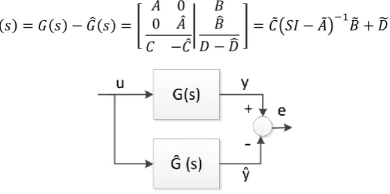
where . The error system is the difference between these two systems which should be minimized. The block diagram of this problem is shown in Fig. 1, and the error system transfer function can be written as follows [15]:
̃( ) ( ) ̂( ) [ ̂ ̂
| ̂
̂
] ̃( ̃) ̃ ̃ (4)
Fig. 1. Error system transfer function
The goal of model order reduction is to find ̂, ̂, ̂ and ̂ such that the infinity norm of the error system is minimized. It can be shown that ‖ ‖ is equivalent to the existence of a symmetric, positive definite matrix satisfying:
[
]
(5)
This inequality is called the bounded real lemma and is proposed in [23]-[25].
In previous model reduction researches, the norm of the error system is minimized by (5) and the best reduced order model is developed. However, the minimum phase characteristic of the reduced system is not regarded. In this paper, a constraint is added to the above minimization problem to guarantee that the minimum phase characteristic of the system is kept unchanged after model order reduction. To achieve this, a special state space representation is exploited which is explained in the next sub-section.
b) LMI constraint to preserve the minimum phase characteristic of the system
To preserve the minimum phase property of the main system, poles and zeros of the reduced system transfer function must be at LHP. It is very easy to apply a LMI condition to force the poles of the system to be at LHP, however, the same cannot be applied to zeroes easily. Thus, the state-space representation has to be defined in a way that conditions on the poles and zeros of the reduced system can be applied. The main idea of the following state space realization is derived from [26].
( )
( ) ( )
(6)
where , , and is the coefficient of when the coefficient of is equal to one ( ). The relative degree . By Euclidean division, ( ) can be written as:
( ) ( ) ( ) ( ) (7)
where ( ) and ( ) are remainder polynomial and the quotient, respectively. It is obvious that the first coefficient of ( ) is ⁄ . From (7), we know that:
(8)
We can rewrite ( ) as follows:
( ) ( )
( ) ( ) ( )
( )
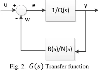
( ) ( ) ( ) (9)
Thus, ( ) can be represented as a closed loop system shown in Fig. 2. The r-th order transfer function ( )⁄ has no zeros, and can be realized by the r-thorder state vector:
( )
[ ̇ ( )] (10)
Therefore, the state space model for ( )⁄ will be:
̇ ( ) (11)
where ( ) is a canonical form representation of a chain of integrators, that is:
[
]
[ ]
[ ] (12)
[
]
(13)
The minimal realization of ( ) ( )⁄ transfer function can be written as:
̇ (14)
December 2015 IJST, Transactions of Electrical Engineering, Volume 39, Number E2 Fig. 2. ( ) Transfer function
The eigenvalues of are the zeros of the polynomial ( ), which are the zeros of the transfer function ( ). Considering and combining (14) and (11), we can write the state-space model of ( ) as:
̇
̇ (15)
where , .
Finally, a new representation of ( ) ( ) is defined where the state-space matrices are:
[ ] [ ] [ ] (16)
Since the eigenvalues of are the zeros of the transfer function ( ), it is necessary to apply the following matrix inequality to be sure that the system zeros are at the LHP.
(17)
Similarly, the following matrix inequality guarantees the stability of the system by forcing the system poles to be at the left half plane.
(18)
3. MODEL ORDER REDUCTION ALGORITHM CONSIDERING THE MINIMUM PHASE PROPERTY OF SYSTEM
Suppose that the main system is ( ) and the reduced order model is defined by ̂( ). In addition, the state space representations of both systems are based on (15). As stated before, the model order reduction problem can be considered as an optimization problem, i.e. minimize ‖ ̃‖ ‖ ̂‖ with respect to
̂. The minimization problem is given below:
Find the smallest possible with respect to ( ̂ ̂ ̂ ̂ ) such that:
[
̃ ̃ ̃ ̃
̃ ̃
̃ ̃
] (19)
and
̂ ̂ (20)
where
̂ [ ̂ ̂ ̂
̂ ̂ ̂ ̂ ̂ ̂ ] (22)
The state space representation of the error system is as follows:
[ ̃ ̃|
̃ ̃ ] [
̂ ̂
| ̂
̂
] (23)
where
̃ [ ̂
̂ ̂ ̂
̂ ̂ ̂ ̂ ̂
] ̃ [
̂ ̂
] ̃
[ ̂ ] ̃
(24)
We can partition matrix and insert (24) into (19) to acquire the final matrix inequality.
Note: in the reduced system, matrices ̂ , ̂, ̂ are known based on (12) and their dimensions depend on the order of the reduced system. ̂ can be chosen arbitrarily. After solving the optimization problem, ( ̂ ̂ ̂ ̂) are obtained.
If the matrix inequality constraints (20) and (21) are satisfied, then the minimum phase property of the reduced system is guaranteed. In other words, inequality (20) causes the real part of the eigenvalues of
̂ to be negative. As a result, the zeros of ̂( ) are at LHP. Similarly, inequality (21) causes the poles of
̂( ) to be at LHP. Thus, the reduced system ̂( ) is minimum phase and the aim of the paper is satisfied.
The matrix inequalities (19)-(21) are not linear matrix inequalities because of the bilinear terms. Thus, LMI methods cannot be applied to find a solution. Suggested solution is to change nonlinear problem into two simpler optimization procedures which are linear in decision variables.
An iterative two-step algorithm can be used as follows:
(1) Find an initial estimation for ̂( ) from other classical techniques. (2) Choose an initial, arbitrary and proper upper bound ( ) for gamma.
(3) Keep ( ̂ ̂ ̂ ̂) constant and minimize with respect to ( ) subject to inequalities (19)-(21) and (25):
(25)
(The optimum computed in this step is used as the initial for next step).
(4) Keep ( ) constant, minimize with respect to ( ̂ ̂ ̂ ̂) and subject to inequalities (19)-(21) and (25). (The optimum computed in this step is also used as initial for step 3)
(5) Repeat steps 3 and 4 until the difference between and is less than a prescribed tolerance .(i.e. stopping condition is | | )
December 2015 IJST, Transactions of Electrical Engineering, Volume 39, Number E2
̂( )‖ ( ) ( ( ) ̂( )) ( )‖ (26)
where ( ) is the input frequency weight and ( ) is the output frequency weight.
4. SIMULATION RESULTS
In this section, two examples are presented to illustrate the performance of the proposed method. In the first example, a 4th-order system is reduced to 3rd and 2nd order models, respectively. In the second example, the LMI based method of this paper is compared to Hankel model order reduction method. The corresponding algorithm has been solved using the MATLAB LMI toolbox [27].
a) Example 1: A 4TH order system
Consider the minimum phase fourth-order system:
( )
(27)
In this system, . Now, we try to reduce this system to a 3rd-order system where
. Based on the expressed state-space realization in section 2.2:
( ) ( )
( ) (28)
Therefore, the following matrices are known:
(29)
[ ] [ ] [ ] (30)
In the reduced model, we have:
̂ ̂ ̂ ̂ (31)
The results which are achieved after running the iterative minimization algorithm are as follow:
̂ * + ̂ * + ̂ [ ] ̂ (32)
( ̂ ) (33)
In Fig. 3, frequency response of the main system and the reduced one are plotted. According to the figure, it is obvious that the minimum phase characteristic of the system is preserved and the bode plot of the main system and the estimated one are close to each other. The main system is also reduced to a system of order 2. The result is as follows:
̂ ̂ ̂ ̂ (34)
( ̂ ) (35)
Fig. 3. Original system versus reduced system of order 3
Fig. 4. Original system versus reduced system of order 2
b) Example 2: A 3RD order system
The purpose of this example is to compare the performance of Hankel model order reduction and the method used in [15] with the proposed order reduction method of the present paper.
In [15], the following minimum phase transfer function is considered:
( )
(36)
At first, the reduced model of order 2 is obtained using Hankel order reduction and the LMI based methods introduced in this paper. Then, the system is reduced to a first order model. The Hankel order reduced model is obtained using MATLAB –Analysis and Synthesis Toolbox [28]:
̂( )
(37)
where the Hankel singular values are 0.7144, 0.191, 0.1017. The error bound of the Hankel model order reduction is ∑ , where the sum is taken over the removed states. It is obvious that the above reduced model is non-minimum phase. The next step is to apply the suggested method to obtain a reduced system of order 2 that preserves the minimum phase characteristic of the system. The following matrices are known according to the system transfer function.
(38)
* + * + [ ] (39)
̂ ̂ ̂ ̂ (40)
The result of the minimization problem is as follows:
̂ ̂ ̂ ̂ (41)
( ̂ ) (42)
December 2015 IJST, Transactions of Electrical Engineering, Volume 39, Number E2
̂( )
(43)
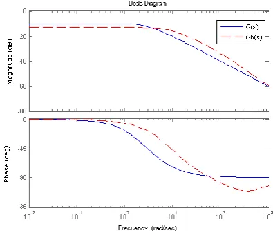
The error bound of the method is 0.1092 which is approximately half of Hankel model order reduction method. In Fig. 5, the frequency response of Hankel reduced model is compared to the LMI based reduced model proposed in this paper. The system is also reduced to a first order model. The Hankel reduced order model is:
̂( )
(44)
The error bound of the above model is 0.5857. It is noticeable that the first order reduced model obtained in [7] is non-minimum phase. The model is as follows:
̂( )
(45)
In this paper, the first order model approximation is found in way to have a minimum phase system. Since the first order reduced system is strictly proper, there are no zeroes in the reduced model. Thus, we have ( ) ( ) and the only decision variable of the minimization problem is ̂.
̂ ̂ ̂ ̂ (46)
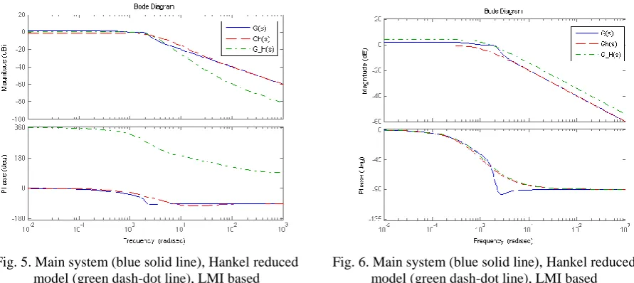
The reduction problem is solved with error bound of 0.5296 and ̂ is obtained. Thus, the following reduced model is achieved:
̂( )
(47)
The frequency responses are shown in Fig. 6. The error bound of the methods illustrated in example 2 is reviewed briefly in Table 1.
Fig. 5. Main system (blue solid line), Hankel reduced model (green dash-dot line), LMI based
reduced model (red dash line)
Fig. 6. Main system (blue solid line), Hankel reduced model (green dash-dot line), LMI based
reduced model (red dash line)
Table 1. error bound of Hankel method versus the LMI approach
5. CONCLUSION
In this paper, model order reduction is defined as an optimization problem. The matrix inequality approach is used to minimize the -norm of the difference between the original system and the reduced one.
The main point of the paper is to propose an extra matrix inequality constraint to guarantee that the minimum phase characteristic of a system is preserved after reduction. To handle it, a special state-space realization of the system is used to be able to apply a condition on the zeros of the reduced system.
This problem was not a linear matrix inequality because of bilinear terms. As a solution, two steps iterative schemes are used to change nonlinear problem into linear matrix inequality. Then, the method is applied to some examples and its efficiency is shown. It is seen that the Hankel order reduced model is non-minimum phase in some cases, while the LMI based method of this paper insures that the minimum phase characteristic of the main system preserves.
The main drawback of iterative LMIs is that we cannot guarantee that the solution converges toward the global minimum. Moreover, a priori knowledge of the variables is required. Obtaining a non-iterative -based model reduction algorithm under the proposed matrix inequality constraint is suggested as the future work of the present paper.
REFERENCES
1. Nasiri Soloklo, H., Hajmohammadi, R. & Farsangi, M. M. (2015). Model order reduction based on moment matching using Legendre wavelet and harmony search algorithm. Iranian Journal of Science and Technology,
Transactions of Electrical Engineering, Vol. 39, No. E1, pp. 39–54.
2. Spanos, J. T., Milman, M. H. & Mingori, D. L. (1992). A new algorithm for optimal model reduction.
Automatica, pp. 897–909.
3. Kabamba, P. T. (1985). Balanced gains and their significance for model reduction. IEEE Transactions on Automatic Control, Vol. 30, pp. 690–693.
4. Pernebo, L. & Silverman, L. M. (1982). Model reduction via balanced state space representations. IEEE Transactions on Automatic Control, Vol. 27, pp. 382–387.
5. Meyer, D. G. & Srinivasan, S. (1996). Balancing and model reduction for second-order form linear systems. IEEE Transactions on Automatic Control, Vol. 41, pp.1632–1644.
6. Skogestad, S. & Postlethwaite, I. (1998). Multivariable feedback control, analysis and design. New York: John Wiley & Sons. Hall.
7. Glover, K. (1984). All optimal hankel-norm approximations of linear multivariable systems and their -error bounds. International Journal of Control, Vol. 39, No. 6, pp. 1115–1193.
8. Enns, D. (1984). Model reduction with balanced realization: an error bound and a frequency weighted generalization. IEEE Conference on Decision and Control, Las Vegas, pp. 127–132.
9. Liu, Y. & Anderson, B. D. O. (1989). Singular perturbation approximation of balanced systems. International Journal of Control, Vol. 50, No. 4, pp. 1379–1405.
10. Sreeram, V. & Agathoklis, P. (1989). Model reduction using balanced realizations with improved low frequency behavior. System & control letters, pp. 33–38.
11. Yan, W. Y. & Lam, J. (1999). An approximate approach to optimal model reduction. IEEE Transactions on Automatic Control, Vol. 44, No. 7, pp. 1341–1358.
12. Boyd, S., Ghaoui, L. E., Feron, E. & Balakrishnana, U. (1994). Linear matrix inequalities in system and control theory. Society for industrial and applied mathematics, Vol. 15.
December 2015 IJST, Transactions of Electrical Engineering, Volume 39, Number E2 14. Valentin, C. & Duc, G. (1997). LMI-based algorithm for frequency weighted optimal -norm model reduction.
IEEE Conference on Decision and Control, pp. 767–772.
15. Helmersson, A. (1994). Model reduction using LMIs. IEEE Conference on Decision and Control,Lake Buena Vista, pp. 3217–3222.
16. Nobakhti, A. & Wang, H. (2009). Noniterative -based model order reduction of LTI systems using LMIs.
IEEE Transactions on Control Systems Technology, Vol. 17, No. 2, pp. 494–501.
17. Ataollahi, M., Eghrary, H. H. & Taghirad, H. D. (2011). Adaptive Robust Backstepping Control Design for a Non-minimum Phase Model of Hard Disk Drives. Conference of Electrical Engineering, Tehran, Iran, pp. 1774– 1779.
18. Khademi, G., Mohammadi, H. & Dehghani, M. (2013). LMI based model order reduction considering the minimum phase characteristic of the system. Asian Control Conference, Istanbul, Turkey.
19. Ebihara, Y. & Hagiwara, T. (2004). On model reduction using LMIs. IEEE Transactions on Automatic Control, Vol. 49, No. 7, pp. 1187–1191.
20. Dehghani, M. & Yazdanpanah, M. J. (2005). Model reduction based on the frequency weighted hankel-norm using genetic algorithm and its application to the power systems. IEEE Conference on Control Applications, pp.
245–250.
21. Salim, R. & Bettayeb, M. (2011). and optimal model reduction using genetic algorithms. Journal of the Franklin Institute, pp.1177–1191.
22. Molagharebagh, M. H. & Dehghani, M. (2011). Frequency weighted model reduction using LMIs.
Conference on Electrical Engineering, Tehran, Iran, pp. 1997–2001.
23. Scherer, C. & Weiland, S. (2004). Linear matrix inequalities in control. Lecture Notes, Dutch Institute for Systems and Control, Delft, The Netherlands.
24. Khargonekar, P. & Zhou, K. (1988). An algebraic riccati equation approach to optimization. System and Control Letters, Vol. 11, pp. 85–91.
25. Willems. J .C. (1971). Least square stationary optimal control and the algebraic riccati equation. IEEE Transactions on Automatic Control, Vol. 16, pp. 621–627.
26. Khalil, H. (1996). Nonlinear Systems. 2nd Edition, Prentice Hall.
27. Gahinet, P., Nemirovski, A., Lab, A. J. & Chilali, M. (1995). LMI control toolbox for use with MATLAB, LMI lab user’s guide. The Mathworks Inc.
28. Balas, G., Doyle, J., Glover, K., Packard, A. & Smith, R. (1993). –analysis and synthesis toolbox for use with
MATLAB, user’s guide. The Mathworks Inc.