Kalman Filter-Smoothed Random Walk Based Centralized Controller for Multi-Input Multi-Output Processes

Vol. 2, No. 2, pp. 155-166, April (2019)

Kalman Filter-Smoothed Random Walk Based Centralized

Controller for Multi-Input Multi-Output Processes

Hamid Fasih

1

, Saeed Tavakoli

2,†

, Jafar Sadeghi

3

and Hamed Torabi

4

†,1,2,4 _{Faculty of Electrical and Computer Engineering, University of Sistan and Baluchestan, Zahedan, Iran} 3 _{Department of Chemical Engineering, University of Sistan and Baluchestan, Zahedan, Iran}

In this paper, a novel centralized controller is presented to control multi-input multi-output industrial processes with heavy interactions and significant time-delays. The system model equations are represented in a non-minimal stochastic state-space form. Also, the state and measurement equations respectively use smoothed random walk model and finite impulse response model of the plant. To design the controller, a quadratic cost function is considered. A standard Kalman filter algorithm is used to estimate the state vector of the controller and solve to the discrete algebraic Riccati equation simultaneously. By using the smoothing parameter, the controller behavior can be changed between the Kalman filter random walk controller and the Kalman filter integrated random walk controller. To evaluate the effect of the smoothing parameter the proposed controller is first applied to a single input single output system. Then an industrial-scale polymerization reactor which has the two-input and two-output system is used to investigate the performance of the designed controller. The simulation results indicate that the controller has a good performance in tracking the set point and robust due to changing the system parameters.

Article Info

Keywords:

Centralized controller, Industrial Scale,

Polymerization reactor, Kalman filter algorithm,

Smoothed random walk model.

Article History:

Received 2018-07-24

Accepted2018-11-12

I.

INTRODUCTION

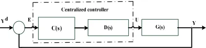
The majority of industrial processes are inputs multi-outputs (MIMO) systems. They have high interaction between inputs and outputs. To cope with this problem, the MIMO system controller is designed in two major categories; decentralized or centralized controller based on the amount of interaction which exists in the process. If the interactions between the different loops of the process are modest, the decentralized controller can work well. It is widely used in the industry due to its proper operation and simply [1-3]. In the control literature, a large number of methods have been reported to design the decentralized controller. Such as detuning method [4], sequential loop closing method [5, 6], relay auto-tuning method [7], and independent design method [8, 9]. If there is heavy interaction in the loops of the process, a centralized controller is advised. The centralized controller changes all inputs to the process simultaneously to accommodate the outputs at their desired values. So, it improves the performance of the MIMO system. These controllers are designed in two different approaches. The first

approach is shown in Fig.1, where G(s), D(s) and C(s) are the process matrix, the decoupling matrix, and the decentralized control matrix, respectively. The second approach is shown in Fig. 2, where G(s), and k(s) are the process matrix and the centralized control matrix, respectively [8]. The decoupled part, in the Fig.1, is used to eliminate the interaction which exists in a different channel of the process. As a result, the controller looks like a completely independent process. Therefore, the controller can be designed with decentralized controller design methods. A simple structure for controlling the MIMO systems is shown in Fig. 2, which does not need the decoupling part. In this structure, the controller matrix must be calculated directly [10]. In this way, all the loops are considered together and then the centralized controller is designed. There is the complexity of calculation of the controller matrix depend on the design method. For example, Bhat et al. presented a centralized controller which used the steady state gain matrix with time constant and time delay of the process transfer function [11], V. Vijay Kumar et al., introduced a centralized controller which was designed based on a direct synthesis method. They obtained the inverse of the process transfer function matrix in the direct synthesis method by using the relative gain array concept [12].

A

B

S

T

R

A

C

T

Moreover, the industrial processes have significant time delay due to distance velocity-lags, recycle loops, and delay in measurements of outputs [13, 14]. Many design methods have been proposed to compensate these time delays. [15, 16] Giraldo, S.A., et al based proposed Multivariable Smith predictor based on the decentralized direct decoupling structure[17]. Uncertainty modeling and saturation of the actuators are other necessary factors to be considered in controller design for MIMO industrial process control in real usage. Some ways to deal with uncertainty modeling of the process is studied in [18-20] .Many researchers report significant results in view of actuators saturation in the industrial process [21-23]. To cope these problems Fasih et al., proposed the Kalman filter general random walk (KF-GRW) controller [24]. It was a centralized controller for non-squared MIMO system based on the Kalman filter algorithms and general random walk model in non-minimal (NMSS) stochastic state space form.

In this paper, we introduce another member of these controller family, that it uses the smoothed random walk model for state equation of state space. The Kalman filter smoothed random walk (SRW) controller, has all the KF-GRW controller properties, also, it provides one more degree of freedom. This degree of freedom causes the controller to be adjusted more quickly and simply. In this controller, each loop of the process can be adjusted easily between the KF-RW and KF-IRW controller by choosing the smoothing parameter. So the better performance for the industrial process can be achieved easily.

This paper is organized as follows. In Section 2, the problem formulation is provided. The control low is presented in Section 3. In Section 4, the simulation example is given. Industrial case study results and discussion are provided in Section 5. Finally, the conclusion is given. The Industrial case study matrices of proposed controllers are shown in the appendix.

II. PROBLEM FORMULATION

In this section, the controller state equation of KF_GRW controller [24] is rewritten by SRW model.

A. System state vector

In the NMSS form, the state vector is given directly from the inputs and measured outputs signals of the process[25]. Many different NMSS forms have been suggested for a range of real application areas [26-28]. In this paper, the state vector, according to the inherent characteristics of an industrial actuator, included the control signal and its changes. We

consider a state vector,x(k) consist of the control signal is

defined as an r-dimensional vector

[

1 2

]

( )

k

=

u k u k

( ),

( ),...,

u k

_r

( )

T

u

, and its difference,

( )

k

( )

k

(

k

1)

∇

u

=

u

−

u

−

as shown in Eq. (1).

( ) = [ ( ), ( )]   

(1)

Fig.1. Centralized control schemes with decoupling block

Fig. 2. Purely centralized control system

B. System state space equations

In this paper, the state equation is expressed as a smoothed random walk (SRW) model. Young et al.[29] , and Norton [30, 31] showed that the RW model in GRW model can also be useful in time variable parameter estimation, which the parameter variations are around a given constant mean value. The IRW model in GRW model to be useful when there are expected to be large variations in the parameters. when the mean value of the parameter is slow variation, instead of constant, it better uses the SRW model [29]. It is a compromise between the IRW and RW models, according to

the smoothing parameter 0 ≤ ≤ 1. From the control point

of view, the KF- RW controller behaves like an integral controller and the KF- IRW controller, like a PI controller. The smoothing parameter determines appropriate percentage of the proportional behavior of the controller. This feature can greatly help to fine-tune the control loops of multivariate systems. Moreover the smoothing parameter give a high degree of freedom to the KF-SRW controller. This capability makes, optimization the Q and R matrices, which are used to tune the KF-GRW controller [24], accelerate. We supposed the SRW model uses to the state equation as shown in Eq.(2).

( )

( ) =

1

0 1

( − 1)

( − 1)

+ 01 ( − 1)

(2)

In which ( ) refers to a zero mean, serially uncorrelated

white noise vector with a covariance matrix of Q . In this case, the state equation of the system is described by Eq. (3).

( ) = ( − 1) + ( − 1)      (3)

Where F_α and G denote the state transmission and input

matrices, respectively. To demonstrate the measurement equation, we use the finite impulse response (FIR) model of the plant in the form of Eq. (4) [24].

( ) = !( − 1) + "!( − 2) + ⋯ + %!( − &) (4)

Thus the measurement equation of KF-SRW controller is as

Eq. (5), [24].

'( ) = ( ( ) + )( )

(5)

Where ξ(k ) refers to a zero mean, serially uncorrelated

L is determined by trial and error in such a way that it yields a reasonable description of the dynamic system. The gains

,

1

,

2

,

3

,

L

h h h

…

h

are related to input at sample time T.

The values of the state space matrices are shown in Table 1.

Table 1. Controller matrices

III. CONTROL LOW

In the NMSS representations, the state vector is given directly from the input and measured output signals of the process [32]. It uses the discrete-time system and using the backward time shift. In NMSS representations, if the system is controllable the NMSS variable feedback controller can be implemented straightforwardly, thus it does not need to an observer. Moreover, it more robust to the uncertainty associated with the estimated model of the system [26, 27]. In KF-GRW controller design method, the NMSS representation

uses only theplant input and past sampled values as the state

vector. In this paper the control signal is obtained by using the

control law of the KF_GRW controller [24] with

consideration of the state equations is presented in Eq. (3) as follow:

(6) * ( ) = + (,( − 1) − *( − 1)-)+ + ./.0

1ℎ343 - = 5 (/ + 5*( − 1)5 )6 _{5*( − 1)}

(7)

7

8

( ) = * ( )5 (/ + 5*( − 1)5 )

6

Where 9 is the covariance matrix and :₈( ) is Control

gain matrix (CGM). The first set of members of the state

vector is extracted by theV matrix

( + 1) = ; ( + 1| )

= = [ I 0]

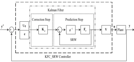
(8)

The KF_SRW closed-loop controller scheme is shown in Fig. 3.

∇e

e d

y y

g

K _{+ z}−1 _{Fα V Plant} +

+_

Correction Step Prediction Step Kalman Filter

SRW

u

KFC_SRW Controller

Fig. 3. The KF_SRW closed-loop control scheme

In Fig. 3, ∇e denote the first differences of the error vector.

For the RW model (α = 0 ), the error vector,

e

is used,

whereas both

e

and ∇e are employed for the SRW model (

0

α > ) or IRW model (α =1).The successive differences ∇e

is used to compensate the added integrals by IRW model

(α =1) or SRW model (0< α <1).

Therefore, the transfer function of the controller in Eq. (9) has only one pole on the unit circle.

( ) = ((? − @

6

)

6

@

6

):

₈

A( )

(9)

IV. SIMULATION EXAMPLE

To evaluate the step response of the proposed control method, the following discrete-time single-input single-output (SISO) system is considered as Eq. (9):

B( ) = C1 −D_{EF B( − 1) + G}HD_{E I( − 1)} (10)

In which the sample time and time constant are T =0.01,

= 1

τ seconds, respectively. Also, the steady-state gain is

1

p

K

=

. The matrices of controllers for state space Eq.(3) and

Eq.(5) are considered as shown in Table 1. In this example,

matrices Q=diag

(

5000,5000

)

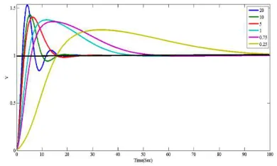
and R=0.01 have been

arbitrarily selected. Fig. 4, shows the unit step responses for the closed loop negative feedback control. system. In this case the is chosen arbitrarily as [0.25, 0.75, 1, 5, 10, 20]. Fig.4.

shows the variations of unit step responses for closed-loop

systems as a function of the . Table 2 shows the p

performance indexes and step response characteristics for the proposed controller. Figs.5-9 show the variation of the closed-loop systems unit step responses characteristics as a function of the .

Table II. The step response characteristics and Performance indexes of the proposed controller according to the

T

α Rise

Time(s)

Settling Time(s)

Over shoot

ξ

_{ITAE IAE}

0.25 11.16 98.25 26.90 0.38 184880 900 0.75 4.10 48.68 35.70 0.31 21962 157 1 3.30 41.83 37.44 0.29 16436 129 5 2.11 23.54 40.34 0.27 186.06 11.41 10 1.89 21.11 42.75 0.26 31.74 5.02 20 1.51 21.44 52.99 0.19 17.94 3.81

α

F

G

H













I

α

0

I

 

 

 

0

I

[

1 2

]

 

 

 

I 0

h h

Fig. 4. The step response of the proposed controller according to changes of the 0 ≤ ≤ 20

Fig. 5. Variation of the rise time of the KF_SRW controller according to changes of the

Fig. 6. Variation of the stelling time of the KF_SRW controller according to changes of the

Fig. 7. Variation of the damping ratio of the KF_SRW controller according to changes of the

Fig. 8. Variation of the performance index (IAE) of the KF_SRW controller according to changes of the

Fig. 9. Variation of the Performance index (ITAE) of the KF_SRW controller according to changes of the

V. INDUSTRIAL CASE STUDY

As an industrial case study we consider an industrial-scale polymerization Reactor (ISPR)[12] The transfer function matrix is given in Eq.(11). It is a two inputs and two outputs squared MIMO system. The relative gain array matrix (RGA) of the ISPR system is given in Eq. (12). The Garish- Gorian bands are plotted in Fig.10.

0.2 0.4

0.2 0.4

22.98

11, 64

4.572

1

1.807

1

( )

4.689

5.8

2.174

1

1.801

1

s s s s

e

e

s

s

G s

e

e

s

s

− − − −



−





+

+







=







+

+







(11)

0.7087 0.2913

0.2913 0.7087





Λ = 







(12)

Fig.10. Garish Gorian bands of the ISPR system

A. KF -SRW controller design

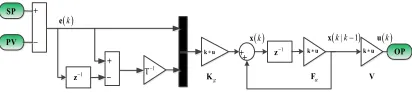
The control objective is set point tracking by a simple and effective centralized controller. The closed-loop control system is demonstrated in Fig. 2. The Simulink diagram of the proposed control method is depicted in Fig. 11 and Fig. 12. The sampling time is T=0.1 second. The matrices of KF-SRW controllers are calculated by Eqs.6, 7 and 8, the values are shown in the appendix.

0 2 4 6 8 10 12 R is e T im e α/T 0 20 40 60 80 100 120

0 5 10 15 20

S et el li n g T im e α/T 0.195 0.245 0.295 0.345 0.395

0 5 10 15 20

0 200 400 600 800 1000

0 5 10 15 20

IA E α/T 0 50000 100000 150000 200000 250000

0 5 10 15 20

IT

A

E

-10 -5 0 5 10

-5 0 5 10

greshgorian band

-10 -5 0 5

-10 -5 0 5 10 Nyquist Diagram Real Axis Im a g in a ry A x is

-1 0 1 2 3

-1 -0.5 0 0.5 1 Nyquist Diagram Real Axis Im a g in a ry A x is

-4 -2 0 2 4 6 8 10

y

Plant

u G0

Step

OP SP

PV Controller

SP PV

IAE y

u

IAE

Fig. 11. KF-SRW control in MATLAB-Simulink

g

K

1

−

z

α

F V

+

+ k u∗ k u∗

∗

k u

( )k

x x(k k|−1)

1

−

z

1

T−

+ _ +

_ PV SP

OP

( )k

e

( )k

u

Fig. 12. KF-SRW control algorithm

To tuning the controller, we minimize the IAE criterion. Q and R matrices are optimized by using simplex methods[33] in MATLAB software. In this example, the starting point of

search, is chosen by tray and error, as Q0= [7, 10, 11.6, 9.35]

and R0= [-8.43, 0.158,-0.011]. The

α

values are chosen as

[0.0, 0.0625, 0.25, 0.5, 1]. The IAE1 and IAE2 values are listed

in Table 3 and the step responses are plotted in Figs. 13-22. The system closed-loop in Fig.11 should be insensitive as possible as to changes in the process model or un-modeled dynamics. To evaluate the robustness of the closed-loop system, we compare the nominal and perturbed systems. In the perturbed system, we consider a %10 increase in steady-state gain and time constant in two separate experiments. Fig.23, and Fig.24.

TABLE III- IAE values for different values.

Fig. 13. Control signals for set point tracking,α = 0

Fig. 14. Output signals for set point tracking,α = 0

Fig. 15. Output signals for set point tracking,α =0 .0 6 2 5

Fig. 16. Control signals for set point tracking = 0.0625

Fig. 17. Control signals for set point tracking, = 0.25

(

α

)

IAE

y

1

y

2

1

1.6 × 10

NO

8.18 × 10

NQ

0.5

70.27

100.9

0.25

19.27

31.90

0.0625 18.68

25.88

Fig. 18. Output signals for set point tracking,α = 0 .2 5

Fig. 19. Control signals for set point tracking, = 0.5

Fig. 20. Output signals for set point tracking, = 0.5

Fig. 21. Output signals for set point tracking,α =1

Fig. 22. Control signals for set point tracking,α =1.

Fig. 23. Compare of the original and perturbed processes after a %10 increase in the steady-state gain

Fig. 24. Compare of the original and perturbed processes after a %10 increase in the time constant

B. PI centralized controller design

We consider the centralized controller introduced in [12] to set point tracking of the ISPR system. The closed-loop control system is shown in Fig. 2. The controller matrix is given in Eq. (15).

( )

0.0688 0.0327 0.2402 0.1073

0.0556 0.0643 0.1792 0.0838

c

s s

G s

s s

 _{+ +} 

 

=  

_{− − +} 

 

  (15)

Using MATLAB-Simulink, the centralized controller is applied to the ISPR. The outputs signals are shown in Fig. 25. Also, the control signals are demonstrated in Fig.26. The,

Fig. 25. Output signals for set point tracking

Fig.26. Control signals for set point tracking

VI.DISCUSSION

In the SISO system, the rise time, settling time and of the

slow response are 11.167 seconds, 98.25 seconds and 0.25

respectively as shown in Fig.4, and Table 2,. Whereas the rise

time, settling time and of the fast response are 1.52 seconds,

21.45 seconds and 20 respectively. Thus rise time and settling

time of the unit response decrease quickly by increasing the

, which are shown in Fig.5, and Fig.6. Fig.7 shows the

variation of the damping ratio (R) of the KF-SRW controller

according to changes of the . It means that the overshoot of

the unit step response increased by decreasing the Table 2

shows that the overshoot of the fast step response is about two times of the overshoot of the slow step response (52.99 against to 26.9). It can be seen from Table 2, that the IAE and ITAE

values are decreased by increasing the . For example, the

fastest and slowest IAE and ITAE of the unit step responses, are reduced by 237 and 10305 times respectively, the variation of these criteria are plotted in Fig.8, and Fig. 9. As a result, if

the matrices S and T are fixed, the controller behavior will be

adjusted by the smoothing parameter.

In the ISPR system, the value of U (0) and U_""(0) in the

RGA(0) matrix in Eq. (12), are 0.708 .These values are

smaller than one. The Garish- Gorian bands in Fig.10, are covered the -1+0j points. So there is an interaction between the system loops. If we closed the second loop, the gain between y1 and u1 will be increased. This it means that the

two loops are not decoupled. The control objective is set point tracking by a purely centralized controller.

The KF-SRW controller is applied to the ISPR system as shown in Fig.11. The IAE criteria of the closed - loop ISPR system are listed in Table3. In the first row of this Table, the smoothing parameter is equal to one. It means the KF-SRW controller is like as KF-IRW controller. The IAE criteria y1

and y2 are 1.6 × 10NO and 8.18 × 10NQ respectively. These

values are very high. Moreover, the control signals in Fig. 21, and the output signals in Fig. 22, show that the closed- loop system is unstable. Thus this value of, the smoothing parameter is undesirable. With decreasing the smoothing parameter about 50%, the IAE criteria y1 and y2 are acceptable (IAE y1= 70.27 and IAE y2 =100.9). In this case, Fig.19, and Fig. 20, illustrate the output signals and the control signals. Many fluctuations exist in these figures show that the

= 0.5 is undesirable as well as. By selecting the value of 0.25 for the smoothing parameter the IAE criterions decrease to 19.27 and 31.90 for y1 and y2 respectively. Fig. 18, shows

the output signals of the ISPR process subject to = 0.25. In

this case the control signals which are shown in Fig. 17, can control the ISPR process, but it is not very soft. We found 0.0625 for the smoothing parameter by tray and error. It can be seen from Fig. 15, and Fig. 16, that the outputs signals and control signals are soft. The IAE criteria y1, 3% and y2, 18%

are less than the = 0.5 IAE criteria’s. In the last row of

Table 3, the smoothing parameter is equal to zero. It means the KF-SRW controller is like as KF-RW controller. Fig. 13, and Fig. 14, show the output signals and control signals respectively.

They are soft. The IAE criteria’s y1 is equal to 20.73 and is

equal to 27.68 for y2, which is 10% higher than the =

0.0625. IAE criteria’s .So, to use the benefits of the KF-SRW

controller and to have a soft control signal, we select the =

0.0625. The S and T matrices were optimized based on this smoothing parameter. They show in the appendix. Tuning the KF- SRW controller with these values are shown that the outputs of the closed loop system track the set point variation at 5 seconds. The controller signal represents a lower control effort for these outputs. Fig. 23, and Fig. 24, show the nominal

and perturbed systems, as they show, they are matched.

Therefore, the controller has a desirable robustness.

To compare the above results, we consider the V.V.Kumar proportional integral centralized controller. The controller matrix is given in Eq. (15). Fig. 25, and Fig. 26, show output signals and Control signals for set point tracking of the ISPR process respectively. The fall time of control signal u1 is 0.17 second at t=0 second and about zero at t=15 second. The rise time of control signal u2 is 0.77 second at t=0 second and about zero at t=15 second. As result, the output signals y1 and y2 have risen time 0.48 second and 0.59 second in t=0 second and t=15 second respectively. To compare this results with the

behavior of KF-SRW controller ( = 0.0625) plot Fig. 27,

that the centralized controllers proposed by V.V.Kumar have undershot about %85 and overshoot about %53 higher than the KF-SRW controller. Thus the Interaction is much decreased in the KF-SRW controller. This is because the control signal considers as time variable parameter in the KF-SRW controller. Fig. 27, shows the control signals of the ISPR by V.V.Kumar controller and the KF-SRW controller together. Fig. 30, compare the control signal rise time values which are listed in Table 5. It can be seen that the rise time of centralized controllers proposed by V.V.Kumar about %60 to %72 is lower than the KF-SRW controller in t=0. In t=15.The rise time of centralized controllers proposed by V.V.Kumar is about zero. Fig. 31, compare control signal peak values which are listed in Table 5. It can be seen that the peak of the control signal of centralized controllers proposed by V.V.Kumar is much higher than the peak of the control signal of the KF-SRW controllers. (About 11 times in t=15). These results show that the KF-SRW controllers produce a smooth control signal and, hence, control valves used in the process remain safe. For quantitative performance measurement, the IAE, values are obtained. The minimize values of IAE for two outputs are 18.68, 25.88 for KF –SRW controller. The IAE values for V.V.Kumar controller are 18.02 and 16.25. Although the V.V.Kumar controller IAE, y2 is 37% less than the SRW controller IAE y2, as Fig 27, show that, the KF-SRW controller produces the soft control signal.

Fig.27. Control signals for set point tracking KF-SRW method and V. Kumar method

Fig.28. Output signals for set point tracking KF-SRW method and V. V.Kumar method

TABLE IV- Output signal information

Controller

Rise

time Peak

time

Settling

time

peak

t 0-15 (second)

PI y1 0.48 0.97 14.32 2.970 y2 -0.43 1.08 6.67 -3.2

KF-SRW y1 0.80 1.27 3.43 1.37 y2 -0.36 1.136 5.197 -0.5

t 15-30 (second)

PI y1 1.09 17.13 26.73 2.7 y2 0.59 16.81 26.35 3.186

KF-SRW y1 0.46 16.24 21.05 1.516 y2 1.92 18.66 20.59 1.076

Table V - Control signal information

Controller

Rise

time Peak

time

Settling

time

peak

t 0-15 (second)

PI u1 0.77 1.11 3 -0.17 u2 -0.17 0.40 8.2 -0.02

KF-SRW u1 1.97 2.80 3.7 0.032 u2 -0.62 0.89 2.9 -0.10

t 15-30 (second)

PI u1 0.00 15.4 18.77 -0.24 u2 0.00 15.19 21 1.16

KF-SRW u1 2 17.55 17.55 0.09 u2 2.92 18 18 0.1

Fig.29. Compare the peak of outputs

Fig.30. Compare the rise time of control signals -4

-2 0 2 4

peak1 peak2

Y1PI Y2PI Y1KF SRW Y2KF SRW

-1 0 1 2 3 4

Risetime1 Rise time2

Fig.31. Compare the peak of control signals

VII. CONCLUSION

The KF-GRW controller was presented in [24] can control the non-squared MIMO system simplify. In this paper we presented one of the members of KF-GRW controller. This controller is a compromise between the KF- IRW and KF-RW controller, by using the smoothing parameter. In this controller, each loop of the process can be adjusted easily between the KF-RW and KF-IRW controller by choosing the smoothing parameter. Moreover, the control system considers dynamic interactions effects instead of steady-state interactions by using SRW model for the control system. So the better performance for the industrial process can be achieved easily. KF-SRW controller was applied to the ISPR system, which has 2 inputs and 2 outputs and compares results with an analytic PI centralized controller, that was presented in [12]. The KF-SRW controller tunes optimally by the

weighting matrices Q, R and smoothing parameter ( ).

According to simulation results, the KF-SRW controller performed satisfactorily in set point tracking for the given industrial case study. The closed-loop control system was robust against the model uncertainties. As the comparison, the KF-SRW controller with PI centralized controller shows that KF-SRW controller doesn’t need to heavy computation. Moreover, the KF-SRW controller produces a smoother control signal than the PI centralized controller. Thus the actuators in process control system such as control valves stay

safe

.

REFERENCES

[1] Garrido, J., F. Vázquez, and F. Morilla,

Multivariable PID control by decoupling. International Journal of Systems Science, 2016. 47(5): p. 1054-1072.

[2] Khaki-Sedigh, A. and B. Moaveni, Control configuration selection for multivariable plants. Vol. 391. 2009: Springer. [3] Xiong, Q. and W.-J. Cai, Effective transfer function method for decentralized control system design of input multi-output processes. Journal of Process Control, 2006. 16(8): p. 773-784.

[4] Luyben, W.L., Simple method for tuning SISO controllers in multivariable systems. Industrial & Engineering Chemistry Process Design and Development, 1986. 25(3): p. 654-660.

[5] Shen, S.H. and C.C. Yu, Use of relay‐feedback test for automatic tuning of multivariable systems. AIChE Journal, 1994. 40(4): p. 627-646.

[6] Wiese, D.P., et al., Sequential Loop Closure Based Adaptive Output Feedback. IEEE Access, 2017.

[7] Nikita, S. and M. Chidambaram, Relay auto tuning of decentralized PID controllers for unstable TITO systems. Indian Chemical Engineer, 2018. 60(1): p. 1-15.

[8] Vu, T.N.L. and M. Lee, Independent design of multi-loop PI/PID controllers for interacting multivariable processes. Journal of Process control, 2010. 20(8): p. 922-933.

[9] Seborg, D.E., et al., Process dynamics and control. 2010: John Wiley & Sons.

[10] Vázquez, F., F. Morilla, and S. Dormido, An iterative method for tuning decentralized PID controllers. IFAC Proceedings Volumes, 1999. 32(2): p. 1501-1506.

[11] Bhat, V.S., I. Thirunavukkarasu, and S.S. Priya, Design of centralized robust pi controller for a multivariable process. Journal of Engineering Science and Technology, 2018. 13(5): p. 1253-1273.

[12] V.V. Kumar, V.S.R.R., M.Chidambaram, Centralized PI controllers for interacting multivariable processes by synthesis method. ISA Transactions, 2012. 51(3): p. 400-409. [13] Gigi, S. and A.K. Tangirala, Quantification of interaction in multiloop control systems using directed spectral decomposition. Automatica, 2013. 49(5): p. 1174-1183.

[14] Shinde, D., S. Hamde, and L. Waghmare, Predictive PI control for multivariable non-square system with multiple time delays. International Journal for Science and Research in Technology, 2015. 1(5): p. 26-29.

[15] Molnár, T.G., et al., Application of predictor feedback to compensate time delays in connected cruise control. IEEE Transactions on Intelligent Transportation Systems, 2018.

19(2): p. 545-559.

[16] Deng, W., J. Yao, and D. Ma, Time‐varying input delay compensation for nonlinear systems with additive disturbance: An output feedback approach. International Journal of Robust and Nonlinear Control, 2018. 28(1): p. 31-52.

[17] Giraldo, S.A., et al., A method for designing decoupled filtered Smith predictors for square MIMO systems with multiple time delays. IEEE Transactions on Industry Applications, 2018.

[18] Wu, Z.-J., X.-J. Xie, and S.-Y. Zhang, Adaptive backstepping controller design using stochastic small-gain theorem. Automatica, 2007. 43(4): p. 608-620.

[19] Tong, S., et al., Adaptive neural network output feedback control for stochastic nonlinear systems with unknown dead-zone and unmodeled dynamics. IEEE transactions on cybernetics, 2014. 44(6): p. 910-921.

[20]Li, Y., S. Sui, and S. Tong, Adaptive fuzzy control design for stochastic nonlinear switched systems with arbitrary switchings and unmodeled dynamics. IEEE transactions on cybernetics, 2017. 47(2): p. 403-414.

[21] Zuo, Z., et al., Event-triggered control for switched systems in the presence of actuator saturation. International Journal of Systems Science, 2018: p. 1-12.

[22] Li, Z., et al., Adaptive robust control for DC motors with input saturation. IET control theory & applications, 2011.

5(16): p. 1895-1905.

[23] Chen, M., S.S. Ge, and B.V.E. How, Robust adaptive neural network control for a class of uncertain MIMO nonlinear systems with input nonlinearities. IEEE Transactions on Neural Networks, 2010. 21(5): p. 796-812. [24] Fasih, H., et al., Kalman filter-based centralized controller design for non-square multi-input multi-output processes.

-0.5 0 0.5 1 1.5

peak1 peak2

Chemical Engineering Research and Design, 2018. 132: p. 187-198.

[25] Wilson, E.D., Q. Clairon, and C.J. Taylor, Stochastic non-minimal state space control with application to automated drug delivery. 2018.

[26] Wilson, E.D., Q. Clairon, and C.J. Taylor, Non-minimal state-space polynomial form of the Kalman filter for a general noise model. Electronics Letters, 2018. 54(4): p. 204-206.

[27] Khalilipour, M.M., et al., Non-square multivariable non-minimal state space-proportional integral plus (NMSS-PIP) control for atmospheric crude oil distillation column. Chemical Engineering Research and Design, 2016. 113: p. 140-150.

[28] Li, H., Tuning of PI–PD controller using extended non-minimal state space model predictive control for the stabilized gasoline vapor pressure in a stabilized tower. Chemometrics and Intelligent Laboratory Systems, 2015.

142: p. 1-8.

[29] Young, P.C., Recursive estimation and time-series analysis: An introduction for the student and practitioner. 2011: Springer Science & Business Media.

[30] Norton, J.P. Identification by optimal smoothing using integrated random walks. in Proceedings of the Institution of Electrical Engineers. 1976. IET.

[31] Brunot, M., et al., An instrumental variable method for robot identification based on time variable parameter estimation. Kybernetika, 2018. 54(1): p. 202-220. [32] Taylor, C.J., P.C. Young, and A. Chotai, True digital

control: statistical modelling and non-minimal state space design. 2013: John Wiley & Sons.

[33] Lagarias, J.C., et al., Convergence properties of the Nelder--Mead simplex method in low dimensions. SIAM Journal on optimization, 1998. 9(1): p. 112-147.

Appendix

The ISPR proposed controller matrices:

1.06

0 -0.06

0

0

0

0

1.06

0 -0.06

0

0

1

0

0

0

0

0

0

1

0

0

0

0

0

0

1

0

0

0

0

0

0

1

0

0

















= 























F

1

0

0

1

0

0

0

0

0

0

0

0

















= 























G

1

0

0

1

0

0

0

0

0

0

0

0

T

















= 























V

1023

-596

-3093 1425

2093 -841

97

295

-296

-708

203

417

0

0

1023 -596

-3093

25

0

0

97

295

-296 -708













=













H

0.0002 0.0005 0.0008 -0.0007 -0.0017 -0.0001 0.0037 0.0002 0 0 0 0 0 0 0 0 0 0

g =

K

0 0 0 0 0 0

 

 

 

 

 

 

 

 

 

 

W = 0.0001 -0.0080

-0.0080 1.2099

1.0000 9.1164 0 0 9.1164 93.9184 0 0 0 0 1 0

0 0 0 1

 

 

 

=

 

 

 

Nomenclature

G Input matrix

e Control error vector

F

Transition matrix

H Measurement equation

h Model parameter

p

K

Gains matrix of plant

g

K

Control gain matrix (CGM)

P

Covariance matrix

Q State vector weighting matrix

R

Error vector weighting matrix

T

Sample time

u

Control signal

X

Vector of states

Y

Vector of outputs

d

Y Vector of set points

Greek Letters

α

Smoothing hyper-parameter ξ Additional noise

ζ Damping ratio

η Input noise vector

θ

Time delay

τ Time constant

∇ Successive differences

Saeed Tavakoli obtained his BSc and MSc degrees from Ferdowsi University of Mashhad, Iran in 1991 and1995, and his Ph.D. degree from the University of Sheffield, England in 2005, all in electrical engineering. In 1995, he joined the University of Sistan and Baluchestan, Iran, where he has been an associate professor since 2011. He has published more than one hundred papers in peer-reviewed journals and conferences. His research interests include the design of classic and fractional-order controllers in the time domain, PID control, control of time-delay systems, optimization, evolutionary algorithms, active and semi-active control of structures, chaos control, robust control, and jet engine control. Dr. Tavakoli serves as the editorial board member for IEEE Transactions on Automation Science and Engineering, Applied Soft Computing, Transactions of the Institute of Measurement and Control, Simulations: Transactions of the society for modeling and simulation. He has served as a reviewer for several journals including IEEE Transactions on Automatic Control, IEEE Transactions on Control Systems Technology, IET Control Theory & Applications, Applied Soft Computing, Journal of the Franklin Institute, Applied Mathematical Modelling, ISA Trans-actions, Applied Mathematics and Computation, Earth-quake Engineering and Engineering Vibration, Computers & Industrial Engineering, Electric Power Components and Systems, Swarm and Evolutionary Computation.

Jafar Sadeghi received the B.S. degree in chemical

engineering from the Isfahan University of

Technology, Isfahan, Iran, in 1991, the M.S. degree in chemical engineering from the Sharif University of Technology, Tehran, Iran, in 1995, and the Ph.D. degree in chemical engineering from the University of Lancaster, U.K., in 2007. He is currently an Associate Professor with the University of Sistan and Baluchestan, Zahedan, Iran. His research interests cover the process modeling and simulation, process control, process identification, process intensification, automation, and instrumentation

Hamed Torabi received the MSc from the University of Science and Technology of Iran and his Ph.D. from Ferdowsi University of Mashhad, Iran all in Electrical Engineering. He is currently an Assistant Professor with University of Sistan and Baluchestan, Zahedan, Iran. His research interests cover the Estimation and Kalman filter, Identification system and control.

IECO