Space-only hyperbolic approximation of the Vlasov equation

(1)

S. Descombes, B. Dussoubs, S. Faure, L. Gouarin, V. Louvet, M. Massot, V. Miele, Editors

SPACE-ONLY HYPERBOLIC APPROXIMATION OF THE VLASOV EQUATION

N. Pham

1

, P. Helluy

2

et A. Crestetto

3

Résumé. Nous construisons une approximation hyperbolique de l’équation de Vlasov dans laquelle la dépendance dans la variable de vitesse a été supprimée. Le modèle ainsi construit possède des propriétés intéressante de conservation et de stabilité de l’entropie. Il peut-être approché par des schémas classiques de résolution des systèmes hyperboliques. Nous présentons des résultats préliminaires sur des cas tests monodimensionnels classiques en physique des plasmas : amortissement Landau, instabilité double faisceau.

Abstract. We construct an hyperbolic approximation of the Vlasov equation in which the dependency on the velocity variable is removed. The resulting model enjoys interesting conservation and entropy properties. It can be numerically solved by standard schemes for hyperbolic systems. We present numerical results for one-dimensional classical test cases in plasma physics: Landau damping, two-stream instability.

Introduction

The most precise models for plasma physics are based on a kinetic description of the charged particles. It is thus important to provide efficient numerical methods for solving such models. Generally, the particles are described by a distribution functionf. The quantityf(x, v, t)dx dvcounts the particles having a position xand a velocity v at time t in a small volume dx dv in the phase space. The distribution function is solution of the Vlasov equation. The Vlasov equation is coupled with the Maxwell equations governing the electromagnetic field, or with the Poisson equation when only the electric field is relevant.

The main difficulty of a kinetic model is that it is a time-dependent system of PDE, set in a six-dimensional space, which leads to very heavy numerical simulations. In some physical configurations, with a strong effect of particles collisions, it is possible to reduce the complexity and returning to a three-dimensional model, such as the MHD model. But in many cases, when the collisions between particles are negligible, it is necessary to rely on the full kinetic model. This is a key point for understanding turbulence inside tokamak plasmas, for instance.

The Particle-In-Cell (PIC) method (see for instance [3,14]) is a popular method for computing collisionless plasma, because it allows performing simulations in complex configurations with a relatively low amount of memory and CPU ressource. However the PIC method is based on an initial random choice of the particles and thus presents numerical noise. Also, it is difficult to ensure the energy conservation. Therefore, Eulerian methods for solving kinetic equations are becoming more and more popular. They allow a better control of the conservation and numerical errors (for a review of eulerian methods, see [7]). We can mention for instance the semi-lagrangian approach, which relies on a grid of the phase space. With this approach it is possible to perform realistic computations on tokamak core plasmas [10].

In this paper, we propose a general Eulerian approach for solving the Vlasov equation. It is based on the semi-discretization of the Vlasov equation with respect to the velocity variable. In this way, we construct a family of reduced models, depending on the velocity discretization parameter P. For low values of P, we recover fluid behavior, while high values of P allow precise approximation of the kinetic model. For a fixed velocity parameter P, the approximate model is a linear hyperbolic system, with non-linear source terms. It is possible to establish in a very simple way conservation and entropy properties. The unknown depends on space and time instead of the full phase-space variables. These two features leads to a simpler reuse of existing solvers for hyperbolic equations. It is

1_{IRMA, 7 rue Descartes, 67000 Strasbourg, [email protected]} 2_{Inria TONUS, [email protected]}

3_{[email protected]}

c

EDP Sciences, SMAI 2013

(2)

possible to incorporate in this way plasma kinetic models into a general, highly optimized solver. The coupling to other fluid plasma models is also simplified.

We apply our approach to the simple case of the one-dimensional Vlasov-Poisson system. We present numerical results for classical plasma physics test cases.

1. Plasma mathematical model

In the following, we present our approach on the one-dimensional classical Vlasov-Poisson system. But it can obviously be generalized to higher dimensions, relativistic cases and Vlasov-Maxwell systems.

1.1. Vlasov-Poisson 1D model

We consider the Vlasov equation

∂tf+v∂xf+E∂vf = 0. (1) The first unknown is the distribution functionf(x, v, t) that depends on the space variable xthe velocity variable v and the timet. It measures, for instance, the quantity of electrons in a plasma having a velocity v at point x and time t. Therefore, it should be a non negative quantity. The second unknown is the electric field E(x, t). We suppose thatx∈]0, L[ and we consider periodic boundary conditions atx= 0 andx=L

E(0, t) =E(L, t), f(0, v, t) =f(L, v, t).

In principle, we should assume thatv∈]− ∞,+∞[ and that the distribution function vanishes atv=±∞. But for practical reasons, we have to bound the velocity space. We suppose that v∈]−V, V[. The Vlasov equation (1) is a transport equation, we have thus also to apply boundary conditions atv=−V or v=V depending on the sign ofE

E(x, t)>0⇒f(x,−V, t) = 0. (2)

E(x, t)<0⇒f(x, V, t) = 0. (3)

Assuming that the electric potential is also L−periodic, we can assume that the electric field has a zero mean

value _ˆ

x

E= 0. (4)

It is solution of the one-dimensional Poisson equation

∂xE=−1 +

ˆ

v

f dv. (5)

The quantityρ0= 1 corresponds, for instance, to the charge density of the background ions.

We also call the systems (1), (5) the Vlasov-Poisson 1D model. The equations (1), (5) are supplemented by an initial condition

E(x,0) =E0(x), f(x, v,0) =f0(x, v).

In our applications (Landau damping and two-stream instability), this initial condition also satisfies

1 L

ˆ

x

ˆ

v f0= 1,

ˆ

x

ˆ

v

vf0= 0. (6)

Then, we can deduce that these two conditions remain true for all time1

1 L

ˆ

x

ˆ

v f = 1,

ˆ

x

ˆ

v

vf = 0. (7)

Let us recall that property (7) is very specific to the test cases that we compute below. For other classical test cases, such as the bump-on-tail instability test case [6], the property has to be adapted.

1_{In fact this result is true if}_f _{has compact support in}_v_{. In our applications, it is only an approximation. We suppose that we can}

(3)

1.2. Vlasov-Amp`

ere 1D Model

The simulation of the Vlasov-Poisson system requires the resolution of an elliptic equation for the electric poten-tial. In the one-dimensional framework, the equation reduces to (5), which is numerically solved by an FFT-based algorithm. It is interesting to propose an equivalent equation for the electric field, which implies the simple numerical resolution of a local differential equation.

We consider the Poisson equation (5) and take the derivative off with respect tox.Suppose thatf is a function with compact support invand that we can change the order of integration of f, then

∂t(∂xE) = ∂t −1 +

´

vf

⇔ ∂x∂tE =

´

v∂tf = ´_v(−v∂xf −E∂vf) = −∂x

´

vvf

−E´_v∂vf,

by hypothesis,f has a compact support inv, thus

E´_v∂vf = E.[f]v_v=+₌_−∞∞

= 0,

thus, finally, we have

∂x∂tE = −∂x

´

vvf

⇒ ∂tE = −

´

vvf+C(t).

(8)

We integrate now with respect toxthe two sides of this equation for obtaining

ˆ

x

(∂tE)dx=

ˆ x − ˆ v

vf+C(t)

dx.

We have

ˆ

x

(∂tE)dx=∂t ˆ

x Edx

= 0.

Finally, we deduce

C(t) = 1 L

ˆ

x

ˆ

v

vf dvdx= 0.

The equation (8) becomes

∂tE=−

ˆ

v

f vdv (9)

which we call the Amp`ere equation.

We also call the system (1), (9) the Vlasov-Amp`ere 1D model.

2. Velocity basis expansion

(4)

2.1. Continuous interpolation by the finite element method

First, we introduce some notations and recall how is constructed the finite element basis. We consider an arbitrary polynomial degreed. The reference element is defined by

ˆ

Q=]−1,1[. We define thed+ 1 reference nodes by

ˆ

Ni=−1 + 2 i−1

d , i= 1· · ·d+ 1.

We mesh the interval ]−V, V[ withN finite elements (Qi)i=1···N and nodes (Nj)j=1···P. The total number of nodes

in this interval isP=d·N+ 1. In practice, we suppose that the nodes are equally spaced in ]−V, V[

Nj =−V + 2V

dN(j−1).

As usual, in our program, we have a connectivity array for detecting that node Nj is the kth local node of a given elementQi

j = connec(k, i) =k+ (i−1)d, 1≤k≤d+ 1, 1≤i≤N. We also use the notation

Nj =Nk,i and then, elementQi has its support in the interval [N1,i, Nd+1,i].

We construct a transformation τi that maps element ˆQ ontoQi. For this purpose we consider the Lagrange polynomials on ˆE, defined by

ˆ

Lk(ˆv) =Y l6=k

ˆ v−Nˆl ˆ Nk−Nˆl

. (10)

The transformation is then given by

τi(ˆv) = d+1

X

k=1

ˆ

Lk(ˆv)Nk,i. (11)

Because the nodes of the mesh are equally spaced in our application, in practice the transformationτiis linear. We construct the interpolation basis in such a way that each basis function ϕj is associated to a nodeNj of the mesh and satisfies

ϕi(Nj) =δij,

where δij denotes the Kronecker symbol. We recall how to compute the basis function ϕj. Let v ∈]−V, V[. Necessarily,v belongs at least to one finite elementQi. Two cases are possible

(1) NodeNj belongs to finite element Qi, i.e.

∃k, Nj=Nk,i.

Then

ϕj(v) = ˆLk(ˆv), v=τi(ˆv). (12)

(2) NodeNj does not belong to Qi, then

ϕj(v) = 0.

2.2. Application to Vlasov velocity discretization

We suppose that the distribution function is approximated by expansion on the basis{ϕj}j=1···P

f(x, v, t) = P X

j=1

wj(x, t)ϕj(v), (13)

we shall also use the convention of sum on repeated indices

(5)

Because of the interpolation property of the basis{ϕj}j=1···P

ϕi(Nj) =δij,

we have

f(x, Ni, t) = P X

j=1

wj(x, t)ϕj(Ni) =wi(x, t).

Therefore, we can approximate the initial condition in the following way

wj(x,0) =f(x, Nj,0) =f0(x, Nj).

We now describe the weak formulation from which we construct the reduced model. Letf be a solution of the Vlasov equation (1) with the boundary condition defined by (2), (3). We recall that

E+= max(0, E), E−= min(0, E).

Then, for all basis functionϕi, we have

∂t

ˆ

v

f ϕi+∂x

ˆ

v

vf ϕi+E

ˆ

v

∂vf ϕi+ E+

2 f(·,−V,·)ϕ(−V)− E−

2 f(·, V,·)ϕi(V) = 0. (15)

This weak form of the transport equation introduces an upwinding only at the boundariesv=±V. The advantages and drawbacks of this approach are discussed in [9].

If we introduce the expression (14) in the weak formulation (15), we obtain

∂twj

ˆ

v

ϕiϕj+∂xwj

ˆ

v

vϕiϕj+Ewj

ˆ

v ϕiϕ0j

+E

+

2 wjϕj(−V)ϕi(−V)− E−

2 wjϕj(V)ϕi(V) = 0.

We can thus introduce the following matrices of dimensionP×P

M = (

ˆ

v

ϕiϕj), A= (

ˆ

v

vϕiϕj).

B(E) = E

+

2Eϕj(−V)ϕi(−V)− E−

2Eϕj(V)ϕi(V) +

ˆ

v ϕiϕ0j.

We obtain the following equation

M ∂tw+A∂xw+EB(E)w= 0, (16)

in whichwis the vector ofP components

w= (w1, w2, ..., wP)T.

ObviouslyAandM are symmetric matrices andM is positive definite. It is then classical to prove that system (16) is hyperbolic, i.e. thatM−1_A_{is diagonalizable with real eigenvalues [8].}

On the other hand, thanks to an integration by part, we find that

Bij =−Bij if (i, j)= (16 ,1) and (i, j)6= (P, P).

In other words the matrixB is “almost” skew-symmetric.

In addition

ifE >0, B11(E) = 0, BP P(E) = 1

2 (17)

and

ifE <0, B11(E) =−

1

(6)

Multiplying equation (16)bywand integrating inx, we can establish the following energy estimate

d dt

ˆ

x

wTM w=1 2E

−_w2 1−

1 2E

+_w2

P ≤0. (19)

This estimate shows that it is essential to modify the source term matrix ´_vϕiϕ0j

with the correction (17), (18) in order to obtain a stable approximation.

2.3. Practical computation of

M, A, B

2.3.1. Gauss-Legendre integration

The (normalized) Legendre polynomials are defined, forn≥0, by

ln(x) = q

n+1₂

n!2n dn dxn((x

2₋₁₎n₎_.

Thenzeros ofln are distinct and in ]−1,1[. We denote by (ξi)i=1···n the zeros ofln and by

ωi=

−√2n+ 1√2n+ 3 (n+ 1)l0

n(ξi)ln+1(ξi)

the integration weights. Then, we have the quadrature formula

ˆ 1

−1

g(v)dv' n X

i=1

ωig(ξi).

The formula is exact ifgis a polynomial of degree 2n−1.

2.3.2. Computation

Firstly, we observe thatM, A and B are sparse matrices. Indeed, with j1, j2 such thatNj1, Nj2 are not in the

same element, we have

ϕj1(v).ϕj2(v) = 0, v∈]−V, V[

thus

Mj1j2=Aj1j2 =Bj1j2= 0.

More precisely, we can state that M, Aand B are band matrices. The bandwidth is equal to the degreed of the local polynomial interpolation. We only have to take care of the non-zero terms of these matrices.

In order to achieve exact numerical integration, we consider d+ 1 Gauss-Legendre integration points ˆξi on the reference element ˆQ with weights ˆωi. It ensures the correct integration of a polynomial of degree 2d+ 1. Such polynomials arise in the terms´_vvϕi(v)ϕj(v)dv. The algorithm for assembling the matrices is then the following:

(1) We loop on the elements of the mesh, we loop on the local nodes of each element. Using the connectivity array, we construct the shape of the sparse matrices. More precisely, if

j1= connec(k1, i) andj2= connec(k2, i)

then the corresponding (j1, j2) elements in the matrices are6= 0.

(2) We loop again on the elements of the mesh. For each elementQi we perform the following algorithm

do k1=1,d+1 do k2=1,d+1

j1=connec(k1,i) j2=connec(k2,i)

M(j1,j2)=M(j1,j2)+´_v_∈_Q

iϕj1ϕj2

A(j1,j2)=A(j1,j2)+´_v_∈_Q

ivϕj1ϕj2

B(j1,j2)=B(j1,j2)+´_v_∈_Q

iϕj1ϕ

0

j2

(7)

Of course, in this algorithm, the matrices M, A and B are stored in a sparse way, for saving computer memory. The first and last terms of the diagonal ofB have also to be corrected according to (17) and (18).

For computing the integrals overQi, we use the geometric transformationτi and Gauss numerical integration.

ForM, we obtain

ˆ

v∈Qi

ϕj1ϕj2 =

ˆ 1

ˆ

v=−1

ˆ Lk1Lˆk2

dv dˆv

=

ˆ 1

ˆ

v=−1

ˆ Lk1Lˆk2τ

0

i(ˆv)

= d+1

X

l=1

ˆ

ωlLˆk1( ˆξl) ˆLk2( ˆξl)τ 0

i( ˆξl).

ForA, we obtain

ˆ

v∈Qi

vϕj1ϕj2 =

ˆ 1

ˆ

v=−1

vLˆk1Lˆk2

dv dvˆ

=

ˆ 1

ˆ

v=−1

τi(ˆv) ˆLk1Lˆk2τ 0

i(ˆv)

= d+1

X

l=1

ˆ

ωlLˆk1( ˆξl) ˆLk2( ˆξl)τi( ˆξl)τ 0

i( ˆξl).

ForB, we obtain

ˆ

v∈Qi

ϕj1ϕ 0

j2 =

ˆ 1

ˆ

v=−1

ˆ Lk1

d dv

ˆ Lk2

dv dˆv

=

ˆ 1

ˆ

v=−1

ˆ Lk1

d dˆv

ˆ Lk2

= d+1

X

l=1

ˆ

ωlLˆk1( ˆξl)

d dvˆ

ˆ Lk2( ˆξl).

We observe that we can compute and store the values and derivatives of the reference basis functions at the reference Gauss points at the beginning of the computation. In the same way, we can compute the upwind and downwind convection matrices

A± = (

ˆ

v

v±ϕiϕj),

where

v+= max(v,0), v− = min(v,0).

These matrices are used in the upwind scheme below.

In Appendix 1 we give additional details on the storage and assembly of the sparse matricesM, A andB.

3. Finite volume schemes

(8)

3.1. Vlasov equation

We consider a finite volume approximation. We assume that the spatial domain ]0, L[ is split intoNxcells. The cellCi is the interval xi−1/2, xi+1/2

, i = 1..Nx. For practical reasons, we also consider two virtual cells C0 and

CNx+1 for applying the periodic boundary condition. At the beginning of a time step, we copy the values of the

cellCNx to the cellC0,and the values of the cellC1 to the cellCNx+1.The center of the cellCi isxi =i4x−

4x

2 .

The space step is4x=_NL

x.We also consider a sequence of timestn, n∈N,such thatt0= 0 andtn=n4t,where

4t satisfies the following CFL condition

4t=α4x

V , 0< α≤1. We are looking for an approximation of the vectorwin the cellCi

wn

i ' w(x, t), x∈Ci, t=tn

We consider the initial conditionsE0=E(·, t= 0),andf0=f(·,·, t= 0). We recall that thejthcomponent of the

initial condition is given by

(w(x,0))_j = f0(x, Nj)

for eachj= 1· · ·P.

We consider the reduced Vlasov model (16), we have

M ∂tw+A∂xw+EB(E)w = 0

⇒M ∂tw = −A∂xw−EB(E)w

If we denoteS=−EB(E)w, we obtain the following evolution equation

M ∂tw=−A∂xw+S. (20)

We consider a finite volume approximation of (20). We denote by wi(t) a piecewise constant approximation ofw in each cell

wi(t)'w(x, t), x∈Ci.

The numerical flux is denoted by (wa, wb) 7→ F(wa, wb). We obtain the following semi-discrete (in space) approximation

M ∂twi=−

F(wi, wi+1)−F(wi−1, wi)

4x +S(w

n i).

Of course we have also to introduce a time discretization in order to compute

wn_i 'wi(tn), x∈Ci.

3.1.1. First-order Euler method

For the time integration we can consider the classical explicit Euler method, which is of order 1. It reads

Mwni+1−w n i

4t = −

F(wn i,w

n i+1)−F(w

n i−1,w

n i)

4x +S(w

n i)

⇒ wn_i+1 = wn

i −

4t

4x M

−1_F₍_wn

i, win+1)−M−1F(wni−1, win)

+4tM−1_S₍_wn i)

(21)

3.1.2. Second order improved Euler method

A time second order scheme is given by the following algorithm

Mw n+1/2

i −w

n i 4t/2 ,=−

F(w_in, wn_i₊₁)−F(w_in₋₁, wn_i)

4x +S(w

n i),

Mw n+1

i −w n i 4t ,=−

F(wn_i+1/2, wn_i₊₁+1/2)−F(wn_i₋+1₁/2, wn_i+1/2)

4x +S(w

n+1/2

(9)

3.1.3. Numerical flux

We consider the centered or upwind numerical flux. The centered flux is given by

F(wL, wR) =A

wL+wR 2

The upwind flux is given by

F(wL, wR) =A+wL+A−wR.

Of course, the first order explicit Euler integration cannot be used with the centered flux, because the resulting scheme is always unstable.

3.1.4. Implementation aspects

In practice, for saving CPU time and memory, we use two subroutines for computations with the sparse matrices in skyline format. The first one computes the product of a sparse matrix and a vector. The other one is used to solve the linear system (by theLU method)

M w=s,

whereM is also a sparse matrix.

3.2. Amp`

ere equation

We have explained how we evolve the reduced Vlasov equation. We have also to evolve the electric field. We have implemented two methods. The simplest method consists in solving the Amp`ere equation (9). The other method is based on a resolution of the Poisson equation (5).

We first consider the Amp`ere equation

∂tE =−

ˆ

v f vdv.

From the representation (14) forf, we have

´

vf vdv = PP

j=1wj(x, t)

´

vvϕj(v)dv = PP_j₌₁wj(x, t)ζj,

where

ζj=

ˆ

v

vϕj(v)dv.

The vector (ζj)j=1···P is computed with an assembly algorithm and Gauss numerical integration as described in Section 2.3.

For the time integration we use, as for w, the first order scheme or the second order improved Euler scheme. Actually, as it is explained in Section 4.2, we have to modify a little bit the time integration in order to obtain precise results.

3.3. Poisson equation

We can also compute the electric field by solving the Poisson equation (5). As in many other works, we use the FFT (Fast Fourier Transform) algorithm.

We consider the cell-centered electric field approximation (E0, E1, ..., ENx−1). We denote byEbkits DFT (Discrete

Fourier Transform, we denote byI=√−1)

b Ek =

N−1

X

j=0

Eje

−2Iπjk

N _{, k}_{= 0}· · ·_N−₁_,

and the inverse DFT is given by

Ej= 1 N

N−1

X

k=0

b Eke

2Iπjk

(10)

We consider the Poisson equation (5)

∂xE = −1 +

´

vf dv

= −1 +PP_j₌₁wj(x, t)´_vϕj(v)dv = −1 +PP_j₌₁wj(x, t)%j

in which%j =

´

vϕj(v)dv. We can compute%j over each element Qi by the assembly algorithm of Section 2.3. We use the notation

σ(x) =−1 +

ˆ

v

f(x, v,·)dv.

A centered finite-difference approximation of the Poisson equation reads

∂xE(xi)'

Ei+1−Ei−1

24x =σ(xi). (23)

Taking the DFT of the two sides of (23) we obtain

b Ek =

4x Isin2_Nπk

x

b

σk, k6= 0.

And, whenk= 0,we have

b E0=

N−1

X

j=0

Ej= 0, (because of condition (4)).

Of course, we use the efficient FFT algorithm (see [12]) for computing the DFT.

3.4. Electric energy

The electric energy is defined by

Ξ(t) = sˆ

L

0

E(x, t)2_dx.

We approximate it by

Ξ(tn)' v u u t4x

Nx

X

i=1

(En i)2

4. Test cases

For testing our solver, we consider several test cases. The first two tests are designed in order to validate the pure transport in the x or v direction. In particular, we will show that the correction (17), (18) is essential in order to obtain correct results. In our numerical experiments, the discretization parameters areN = 20,d= 5 and Nx= 128.

4.1. The transport equation

Consider the Vlasov equation

∂tf+v∂xf+E∂vf = 0.

If we suppose that∂xf = 0 and the electric field is constant with respect tot, namelyE(x, t) =E(x, t= 0) =E0(x),

thus the Vlasov equation becomes

∂tf+E(x)∂vf = 0, (24) which is av-transport equation.

If we suppose that the electric field vanishes at any time and any position, we obtain thex-transport equation

(11)

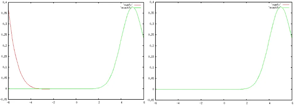
Figure 1. The v-transport for the Vlasov equation after T = 5, we compare the exact solution (green curve) and the numerical solution (red curve). Left: without the correction onB(E). Right: with correction.

4.1.1. The v-transport equation

Consider thev-transport equation (24) with a given initial conditionf0. Thanks to the method of characteristics,

the exact solution is given by

f(x, v, t) =f0(x, v−E(x)t).

Suppose that the initial conditions is given by

• The distribution function

f0(x, v) = (1 +cos(kx))

1 √

2πe

−v2

2 ,

• The electric field

E0(x) = 1,

• The domainL= 2π k .

Let us take the values of parameter k= 0.2 and = 5×10−2_{. The results are given on Figure (1). We compare}

the numerical solution of thev−transport equation and the exact solution. We can see that without the correction (17), (18) the numerical solution is wrong.

4.1.2. The x-transport equation

We consider also the x-transport equation (25) with a given initial condition f0. The exact solution of this

transport equation is given by

f(x, v, t) =f0(x−vt, v).

With the same initial conditionf0 as in thev-transport test, we obtain the result of Figure 2.

4.2. The Landau damping

In this test case, we consider the following initial data

• The distribution function

f0(x, v) = (1 +cos(kx))

1 √

2πe

−v2

2 _,

• the electric field

E0(x) =

(12)

Figure 2. Thex-transport test for the Vlasov equation after T = 20. The exact and numerical curves are superimposed.

For small, thanks to a linear approximation of the non-linear Vlasov-Poisson system, it is possible to compute an approximate analytic solution of the electric field. The details of the computation are given in [13]. The electric field is given by

E(x, t) = 4reωit_sin(_kx_{) cos(}_ω

rt−ϕ), (26)

where ωi, ωr are the real part and the imaginary part of ω, respectively. The numerical values ofω, r and ϕare given in the following table

k ω reIϕ

0.5 0.4 0.3 0.2

±1.4156−0.1533I ±1.2850−0.0661I ±1.1598−0.0126I ±1.0640−5.510×10−5_I

0.3677e±I0.536245 0.424666e±I0.3357725

0.63678e±I0.114267

1.129664e±I0.00127377

In addition, the distribution function can be computed by a well validated method, such as the PIC method. We compare our numerical results with the PIC results and also with the analytic solution.

Firstly, we compare the distribution function of the reduced Vlasov-Poisson method and of the PIC method (taken from [5]). The value of the parameters are k = 0.2 and = 5×10−2. We plot the distribution function computed by the two methods at different times t= 0, t= 10, t= 20, t= 30,t= 40 and at t= 100. The results are on Figure 3, 4, 5, 6, 7 and 8.

The reduced Vlasov approximation satisfies only an L2 stability estimate (19). Such estimate does not ensure the positivity of f. Indeed, in our simulations we observe at some points slightly negative values of f. But the numerical results are anyway very satisfactory. We explain in Appendix 2 how we could avoid negative values off.

We also plot the logarithm of the electric energy in order to compare the reduced Vlasov-Poisson method with the PIC method on Figure 9.

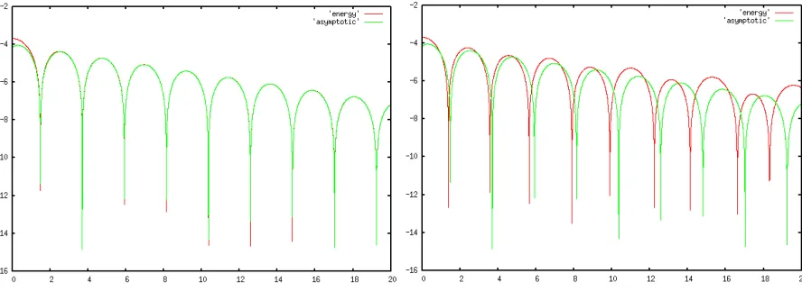
Now, we take the parameters k = 0.5 and = 5×10−3_{. In Figure 10, we plot the logarithm of the electric}

energy computed by reduced Vlasov-Poisson method and by the formula (26). We compare the first and second order schemes. We can see that the second order scheme is more precise than the first order scheme.

(13)

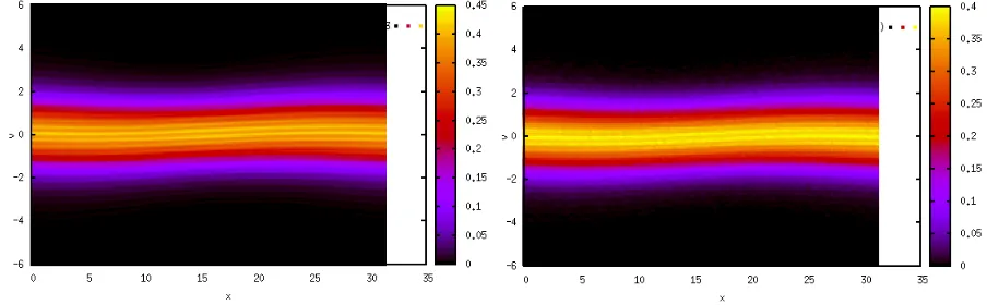
Figure 3. The distribution function of the Landau damping test case at timet= 0. Left: reduced Vlasov-Poisson method. Right: the PIC method.

4.3. Two-stream instability

In this test case, the initial distribution function is given by

f0(x, v) = (1 +cos(kx))

1

2√2π

e−(v−v0 )

2

2 +e−

(v+v0 )2 2

,

(14)

Figure 8. The distribution function of the Landau damping test case at time t = 100. Left: reduced Vlasov-Poisson method. Right: the PIC method.

Firstly, we remark that we have to take the polynomial degree d large enough to reach good precision. For example, Figure 12 represents the distribution function at time t = 25 with the polynomial degree dequals to 4 and 5 respectively. The number of elements here is chosen toN = 20.

We observe a better precision (less oscillations) withd= 5 than withd= 4.

(15)

Figure 9. The electric energy of the Landau damping test case up to timet= 20, the green curve is computed by the PIC method and the red curve is computed with the reduced Vlasov-Poisson method (second order scheme).

Figure 10. The electric energy of the Landau damping test case up to timet= 20, the green curve “asymptotic” is computed with the formula (26) and the red curve “energy” is computed with the reduced Vlasov-Poisson method. Left: Euler scheme with the upwind flux. Right: Rung-Kutta scheme with the centered flux.

(16)

Figure 12. The distribution function of the two-stream test case at timet = 25 computed with the reduced Vlasov-Poisson method with difference parameterd. Left: d= 4. Right: d= 5.

Figure 13. The distribution function of the two-stream test case at timet = 0. Left: reduced Vlasov-Poisson method. Right: the PIC method.

Figure 14. The distribution function of the two-stream test case at time t = 15. Left: reduced Vlasov-Poisson method. Right: the PIC method.

(17)

Figure 18. The distribution function of the two-stream test case at timet = 50 computed with the reduced Vlasov-Poisson method. Left: with the centered flux. Right: with the slightly upwinded flux.

At timet= 50, we observe small numerical oscillations in the reduced Vlasov-Poisson method. These oscillations are due to the fact that we have no upwind mechanism in the resolution of the transport equation with the centered numerical flux.

In order to remove the oscillations in the above test case, we introduce a slightly upwinded flux

F(wL, wR) =A

wL+wR

2 −

ε

2(WR−WL),

whereεis a numerical viscosity parameter. Taking the parameterε= 0.01 and we obtain the distribution function at timet= 50 on Figure 18 in which the oscillations have disappeared.

(18)

entropy estimate. It also allows to construct natural dissipative source term, which can be used for stabilizing the numerical method or for introducing a physical dissipative mechanism, such as collisions effect.

In a forthcoming work, we intend to implement an upwind Discontinuous Galerkin (DG) method in order to introduce dissipation in the numerical method, while keeping high order.

4.4. Computation time

We also compare the computation time of the reduced Vlasov-Poisson method with the PIC method. We consider the following data: Nx = 256,V = 6, Tmax= 20 the CFL α= 0.6 and the parameters k= 0.2 and= 5×10−2

for the landau damping test case. The number of time iteration is 1630. The reduced Vlasov-Poisson computation lasts 13,965 seconds while the PIC computation, with approximately 130,000 particles, lasts 18 seconds. The graph of the electric energy is shown in Figure 9.

5. Conclusion

In this paper, we have constructed a new method for approximating the Vlasov equation. We first performed an approximation in the velocity direction. The resulting system is a first order system of hyperbolic equations. Its convective part is linear while the nonlinearity is concentrated into the source term, which couples the kinetic equation and the electromagnetic field. The solutions satisfy natural conservation and energy estimates. We are also able to provide a nonlinear version of the model, where the distribution function is positive and satisfies a natural entropy estimate.

It is then possible to apply to the reduced Vlasov model the whole range of numerical methods that have been developed for hyperbolic systems. In this paper we compare two classical methods: the upwind first order scheme and a centered second order scheme. We obtain good results on two classical test cases in plasma physics: Landau damping and two-stream instability.

In the future, we plan to extend our method to higher dimensional problems, relativistic particle beams, gyroki-netic plasma approximations and weak collisions models.

Appendix 1: skyline storage of the matrices

For storing a sparse matrixM (orAorB) of size nnoe×nnoe in the skyline format, we use the following arrays: mdiag(1:nnoe) for storing the diagonal, msup(1:nsky) and mlow(1:nsky) for storing the upper and lower parts. The integer nsky is unknown at the beginning. We need also an additional array mkld(1:nnoe+1) for locating the beginning of each column (row) in msup (mlow). We use the convention mkld(1)=1 and mkld(nnoe+1)=nsky+1. In practice, for constructing mkld, we use an intermediate array prof(1:nnoe). prof(i) contains the number of stored elements ofM in column (row) i in msup (mlow). Thus prof(1)=0. For building prof, we use the following algorithm

prof=0 do k=1,nel

do ii=1,d+1 do jj=1,d+1 i=connec(ii,k) j=connec(jj,k)

prof(j)=max(prof(j),j-i) prof(i)=max(prof(i),i-j) enddo

enddo enddo

Once prof is known, mkld is built with the following algorithm

mkld(1)=1 do i=1,nnoe

(19)

At the end of this algorithm, we know nsky=mkld(nnoe+1)-1, we can thus allocate the memory for msup and mlow.

Finally, let (i, j) corresponds to a non-zero element of matrix M (it means that we can find an element indexk and two local node indicesii and jj such thati=connec(ii, k) and j =connec(jj, k). We can recover Mij from the arrays mdiag, mlow, msup, mkld by the following algorithm

if (i.eq.j) then Mij = mdiag(i) else if (j.gt.i) then

Mij = msup(l) with l=mkld(j+1)-j+i else

Mij = mlow(l) with l=mkld(i+1)-i+j endif

The structure of the matrices A, BandM are the same. We have to compute mkld only once.

Appendix 2: Non-linear Vlasov reduction

For improving the dissipation, we consider now a source term in the Vlasov equation. It can represent collisions between particles. The Vlasov equation (1) becomes

∂tf+v∂xf+E∂vf =Q(f), (27)

whereQ(f) is a source term, which we denote by the collision kernel. We also consider an entropyS(f). The entropy is supposed to be a smooth strictly convex function off. In practice, we will consider the following entropies

(a)S(f) =f

2

2 , (b)S(f) =f(lnf −1), (c) S(f) = f2

2 −εlnf, ε >0.

The entropy variable is

g=S0(f).

ConsideringS∗, the Legendre transform ofS

S∗(g) = max

f (gf−S(f)),

we also have

f =S∗0(g).

In the previous sections, we expandedf on an interpolation basis. Now, we expand the entropy variableg in the Legendre basis. A first advantage is that ifS∗0 is positive, the distribution function is automatically positive. It is the case with choice (b) and (c). With choice (a) we recover the reduced Vlasov model of the previous sections because thenS0(f) =g=f.

Suppose that

g(x, t, v) = P X

k=1

gk(x, t)ϕk(v). (28)

We denote by Π the orthogonal projection ofgon a subspaceV0of the interpolation spaceV = span{ϕi, 1≤i≤P}. For a given constantλ >0, we can then consider the collision kernel

Q(f) =λ(Πg−g). (29)

Iff has a compact support inv, we can prove the following results

• ´_vQ(f)ϕdv= 0, ∀ϕ∈ V0.In particular, ifv→vmis in the spaceV0then them−moment off is conserved

in the sense that _ˆ

x

ˆ

v

(20)

• The total entropy Σ =´_vS(f)dvis decreasing

∂tΣ +∂xG(Σ)≤0, withG(Σ) =

ˆ

v vS(f).

The proof is an immediate adaptation of techniques presented in many works on non-linear hyperbolic systems and Boltzmann theory. We refer for instance to [2, 8, 11].

The collision kernel (29) can be used of course for introducing a physical phenomenon. But we can also use it as a numerical tool for damping numerical oscillations. We will investigate this kind of tools in forthcoming works.

References

[1] C. Altmann, T. Belat, M. Gutnic, P. Helluy,H. Mathis, E. Sonnendr¨ucker, W. Angulo, J.-M. H´erard. A local time-stepping dis-continuous Galerkin algorithm for the MHD system. CEMRACS 2008—Modelling and numerical simulation of complex fluids, 33–54, ESAIM Proc., 28, EDP Sci., Les Ulis, 2009.

[2] T. Barth. On discontinuous Galerkin approximations of Boltzmann moment systems with Levermore closure. Comput. Methods Appl. Mech. Engrg. 195 (2006), no. 25-28, 3311–3330.

[3] C. K. Birdsall, A. B. Langdon. Plasma Physics via Computer Simulation. Institute of Physics (IOP), Series in Plasma Physics, 1991. [4] S. Le Bourdiec, F. de Vuyst, L. Jacquet. Numerical solution of the Vlasov-Poisson system using generalized Hermite functions.

Comput. Phys. Comm. 175 (2006), no. 8, 528–544.

[5] A. Crestetto, Optimisation de méthodes numériques pour la physique des plasmas. Application aux faisceaux de particules chargées, her thesis, October 2012.

[6] N. Crouseilles, M. Mehrenberger, E. Sonnendr¨ucker. Conservative semi-Lagrangian schemes for Vlasov equations. J. Comput. Phys. 229 (2010), no. 6, 1927–1953.

[7] F. Filbet, E. Sonnendr¨ucker. Comparison of Eulerian Vlasov solvers Comput. Phys. Commun., 150 (2003), pp. 247–266.

[8] E. Godlewski, P.-A. Raviart. Numerical approximation of hyperbolic systems of conservation laws. Applied Mathematical Sciences, 118. Springer-Verlag, New York, 1996.

[9] C. Johnson, J. Pitk¨aranta. An analysis of the discontinuous Galerkin method for a scalar hyperbolic equation. Math. Comp. 46 (1986), no. 173, 1–26.

[10] G. Latu, N. Crouseilles, V. Grandgirard, E. Sonnendr¨ucker. Gyrokinetic Semi-Lagrangian Parallel Simulation using a Hybrid OpenMP/MPI Programming, Recent Advances in PVM an MPI, Springer, LNCS, pp 356-364, Vol. 4757, (2007).

[11] B. Perthame. Boltzmann type schemes for gas dynamics and the entropy property. SIAM J. Numer. Anal. 27 (1990), no. 6, 1405–1421.

[12] W. H. Press, S. A. Teukolsky, W. T. Vetterling, B. P. Flannery: Numerical Recipes in C.

[13] E. Sonnendr¨ucker Approximation numerique des equations de Vlasov-Maxwell, Notes du cours de M2, 18 mars 2010.