E. Canc`es and S. Labb´e, Editors
NUMERICAL HOMOGENIZATION: SURVEY, NEW RESULTS, AND
PERSPECTIVES
Antoine Gloria
1Abstract. These notes give a state of the art of numerical homogenization methods for linear elliptic equations. The guideline of these notes is analysis. Most of the numerical homogenization methods can be seen as (more or less different) discretizations of the same family of continuous approximate problems, which H-converges to the homogenized problem. Likewise numerical correctors may also be interpreted as approximations of Tartar’s correctors. Hence the convergence analysis of these methods relies on the H-convergence theory. When one is interested in convergence rates, the story is different. In particular one first needs to make additional structure assumptions on the heterogeneities (say periodicity for instance). In that case, a crucial tool is the spectral interpretation of the corrector equation by Papanicolaou and Varadhan. Spectral analysis does not only allow to obtain convergence rates, but also to devise efficient new approximation methods. For both qualitative and quantitative properties, the development and the analysis of numerical homogenization methods rely on seminal concepts of the homogenization theory. These notes contain some new results.
R´esum´e. Ces notes de cours dressent un ´etat de l’art des m´ethodes d’homog´en´eisation num´erique pour les ´equations elliptiques lin´eaires. Le fil conducteur choisi est l’analyse. La plupart des m´ethodes d’homog´en´eisation num´erique s’interpr`ete comme des discr´etisations (plus ou moins diff´erentes) d’une mˆeme famille de probl`emes continus approch´es qui H-converge vers le probl`eme homog´en´eis´e. De mˆeme, le concept de correcteur num´erique s’interpr`ete comme une approximation des correcteurs introduits par Tartar. Ainsi l’analyse de convergence repose essentiellement sur la th´eorie de la H-convergence. Si on s’int´eresse aux estimations quantitatives d’erreur, il faut faire des hypoth`eses suppl´ementaires de structure sur les h´et´erog´en´eit´es (p´eriodicit´e par exemple). Dans ce cas, un outil important est l’interpr´etation spectrale de l’´equation du correcteur introduite par Papanicolaou et Varadhan, qui permet non seulement de d´emontrer des r´esultats quantitatifs, mais aussi de d´evelopper des m´ethodes num´eriques efficaces. Qu’il s’agisse de propri´et´es qualitatives ou quantitatives, le d´eveloppement et l’analyse de m´ethodes d’homog´en´eisation num´erique reposent sur des concepts fondateurs de la th´eorie de l’homog´en´eisation. Ces notes contiennent quelques r´esultats nouveaux.
Contents
1. Introduction 51
1.1. Motivation 51
1.2. Self-consistent approach 52
1.3. H-convergence 55
1
Project-team SIMPAF & Laboratoire Paul Painlev´e UMR 8524 INRIA Lille - Nord Europe & Universit´e Lille 1
Villeneuve d’Ascq, France [email protected]
c
EDP Sciences, SMAI 2012
2. Analytical framework by H-convergence 57
2.1. General framework 57
2.2. Numerical corrector 61
2.3. Direct approach 69
2.4. Dual approach 71
3. Resonance, windowing, and oversampling 74
3.1. Numerical analysis of the periodic case and the resonance error 74
3.2. Windowing and filtering in the direct approach 77
3.3. Oversampling in the dual approach 78
3.4. Analytical framework 79
4. Reduction of the resonance error by zero-order regularization 84
4.1. Description of the method, and analysis in the periodic case 85
4.2. Spectral analysis for symmetric coefficients and consistency in the stationary ergodic case 87 4.3. Convergence rates in the stochastic case with finite correlation-length 91
4.4. Improving the convergence rate by Richardson extrapolation 92
4.5. Numerical tests 94
4.6. Comments on the periodization method 102
5. Numerical homogenization with zero-order regularization 104
5.1. Analytical framework 105
5.2. Direct and dual approaches 109
5.3. Numerical analysis of the locally periodic case 110
5.4. Richardson extrapolation for the numerical corrector 110
6. Other approaches and perspectives 112
6.1. Other approaches 112
6.2. Beyond the linear case 113
6.3. What next ? 114
References 114
1.
Introduction
1.1.
Motivation
Numerical homogenization methods (see [20, 42, 43], [6], [25], [17–19] e.g.) are designed to solve partial differential equations for which the operator is strongly heterogeneous spatially. Such problems arise in many applications such as diffusion in porous media or composite materials. We refer the reader to the bibliography for details on the fields of application. By numerical homogenization, we mean that we compute not only an “averaged” solution of the highly heterogeneous problem, but also the local fluctuations, which may be important in many applications. We focus in this article on the prototypical problem of a scalar linear elliptic equation: for some 1≫ε0>0, finduε0 ∈H01(D) such that
−∇ ·Aε0∇uε0 = f inD, (1.1)
on a Lipschitz domain D for some f ∈ H−1(D). Here, the spatial dependence of the operator is encoded
in the function Aε0, whose frequencies are assumed to be of order ε−01. Academic cases are of the form:
Aε0(x) =A(x/ε0), withAperiodic, quasi-periodic or stationary in an ergodic stochastic setting. More realistic
models can be of the form: Aε0(x) =A(x, x/ε0), whereA(x,·) may be periodic, quasi-periodic or stationary for
allx∈D, provided some suitable cross-regularity holds (see [4] e.g.). In all these examples,ε0refers to theactual
benefit from the structure of Aε0 to design more efficient methods, avoiding the use of fine mesh on the whole domainD.
A first abstract step consists in imbedding (1.1) into a whole family of problems parametrized by ε >0:
−∇ ·Aε∇uε = f in D, (1.2)
and which coincides with (1.1) for ε=ε0. Since ε0 is small, a natural strategy is to pass to the limit asε→0
in (1.2), and solve the limiting problem at “ε= 0” instead of (1.1). Of course, from a practical point of view we are givenAε0 and not necessarily{Aε}ε>0, and althoughε0 is small, it is not zero and one should somehow
remember this scale in the approximation. These two concerns are addressed formally in this introduction. We shall first quickly recall the main results of the H-convergence theory, and then show how to deduce a numerical homogenization procedure from this theory using a “self-consistent” approach.
The rest of this survey is organized as follows. In the second section we introduce more rigorously these numerical homogenization methods, and provide a qualitative convergence analysis using H-convergence. In Section 3 we display a quantitative convergence analysis of the periodic case, putting in evidence the so-called resonance error. We then present two standard ways to reduce the resonance error, windowing and oversampling, and extend the qualitative convergence analysis to these cases. In Section 4 we turn to a more efficient way to deal with the resonance error, based on the introduction of a zero-order term in the corrector equation. We describe the approach on the approximation of homogenized coefficients, and prove the convergence of the method using spectral analysis — which requires the matrix Aε to be symmetric. In Section 5 we combine the numerical homogenization methods with the regularization approach to reduce the resonance error, and introduce another numerical corrector which approximates better the local fluctuations of the solution. We then quickly mention in Section 6 two other numerical homogenization methods based on unfolding and on harmonic coordinates, as well as a small collection of examples illustrating how the strategies developed so far for the linear case can be adapted to the nonlinear case, and why new ideas are definitely needed.
A a general rule, most of the qualitative convergence results are proved in detail. For quantitative results, the proofs are often omitted and precise references are given.
1.2.
Self-consistent approach
In this paragraph we present a formal approach to compute an approximation of the solution of (1.2) which takes advantage of the scale separation ofAε. The justification of this approach will be given in Section 2.
The starting point of the self-consistent approach is the assumption that the solutionuεto (1.2) displays the same scale separation asAε in the sense that it can be decomposed as
uε = uε+ ˇuε,
where
• uεis a low frequency part (say with frequencies of order 1),
• uˇεis a high frequency part (frequencies of order ε−1) possibly modulated by a factor with frequencies of order 1.
In particular, we assume that for every open bounded subdomain T ofD
T ˇ
uε . ε.
Note that the fact that the solution uε to (1.2) displays the same scale separation as Aε may not be true in general. This decomposition can be made explicit in the periodic case using the two-scale expansion [8]
uε(x) = u0(x) +εu1(x,
x
which yieldsuε=u0(x) and ˇuε=εu1(x,xε) +o(ε).
The self-consistent approach consists in deriving equations for uε and ˇuε as consequences of the fact that
uε+ ˇuε is a solution to (1.2). For the reasoning, we letuε,H be an approximation ofuε in some P1-FE space
VH ⊂H01(D) associated with a triangulation{Tk}k ofD of meshsizeH ≫ε, andfH be an approximation of
f in the associatedP0-FE space. We rephrase the question as: What is the link betweenuε,H andAε ? By assumption, uε,H+ ˇuε is a good approximation ofuε in H01(D). In addition, the assumption on ˇuε reads on each elementTk
ˆ
Tk
ˇ
uε = |Tk|O(ε),
which we will assume to be zero forsimplicity of the argument. Inserting “uε=uε,H+ ˇuε” in (1.2), we obtain that ˇuε satisfies for allvε∈H01(Tk)∩L20(Tk) (that is the functions ofH01(Tk) with zero average onTk)
ˆ
Tk
∇vε·Aε∇uˇε = − ˆ
Tk
∇vε·Aε∇uε,H+ ˆ
∂Tk
vεn·Aε∇(uε,H+ ˇuε) + ˆ
Tk fHvε
= −
ˆ
Tk
∇vε·Aε∇uε,H
sincefH is constant onTk and ´T
kvε= 0. Hence, we have
• one equation for ˇuεon each elementTk,
• compatibility conditions for ˇuε on∂Tk (continuity at the interfaces). This couples the scalesεand H at the interfaces
We then make a local closure assumption, and impose ˇuε = 0 on∂Tk — which implies that ˇuε ∈H01(Tk)∩
L2
0(Tk). This decouplesεand H. Indeed, on every elementTk, by the Lax-Milgram theorem, ˇuε∈H01(Tk)∩
L2
0(Tk) is the unique solution to: For allvε∈H01(Tk)∩L20(Tk)
ˆ
Tk
∇vε·Aε(∇uε,H+∇uˇε) = 0.
Define ψk
ε,i ∈H01(Tk)∩L20(Tk) for everyk and every{ei}1≤i≤d (the canonical basis of Rd) as the unique weak solution to: for allχ∈H1
0(Tk)∩L20(Tk),
ˆ
Tk
∇χ·Aε(ei+∇ψkε,i) = 0.
Then by linearity and using that∇uε,H is piecewise-constant:
ˇ
uε= X
k d X
i=1
(∂iuε,H)|Tkψ
k
ε,i∈H01(D).
Hence, setting Ψε=Pk1Tk(ψ
k
ε,1,· · · , ψε,dk )∈H01(D,Rd), we have for allφH ∈VH and all ˇφ∈H01(D) such that
ˇ
φ|Tk∈H
1
0(Tk)∩L20(Tk) for allk,
ˆ
D∇
(φH+ ˇφ)·Aε(Id +∇Ψε)∇uε,H = ˆ
D
(φH+ ˇφ)fH = ˆ
D
φHfH.
This allows us to obtain a closed equation foruε,H by taking ˇφ≡0: For allφH∈VH,
X
k
(∇φH)|Tk
ˆ
Tk
Aε(Id +∇Ψε)
(∇uε,H)|Tk =
ˆ
D
that is
ˆ
D∇
φH·A∗ε,H∇uε,H = ˆ
D
φHf
with A∗ ε,H =
X
k 1|Tk
ˆ
Tk
Aε(Id +∇Ψε). So defined, A∗ε,H is expected to have frequencies of order 1 (or say
H−1 at worst), but notε−1. We then finally obtain
uε≃uε,H+ ˇuε=uε,H+ X
k d X
i=1
(∂iuε,H)|Tkψ
k ε,i.
There are at least two ways to exploit this chain of arguments in practice at ε fixed. We start with the “direct approach”, which appears for instance in [17, 18, 25]. The method is as follows: first approximate Ψk
ε by Ψk
ε,h for allk using a FE method and a fine mesh ofTk (with meshsizeh≪ε), then construct the associated approximation ofA∗
ε,H
A∗ ε,H,h :=
X
k 1|Tk
ˆ
Tk
Aε(Id +∇Ψkε,h),
defineuε,H,has the unique solution inVH to
For allφH ∈VH, ˆ
D∇
φH·A∗ε,H,h∇uε,H,h = ˆ
D
φHf, (1.3)
and finally reconstruct an approximation ofuεvia
uε≃uε,H,h+ X
k d X
i=1
(∂iuε,H,h)|Tkψ
k
ε,i,h. (1.4)
This method amounts to approximating the low frequency partuεofuε, and to reconstructing the high frequency part ˇuε afterwards. Hence the equation is changed (Aε is replaced byA∗ε,H,h), but the finite element space is the coarse spaceVH (withH ≫ε).
We now turn another point of view, which we call the “dual approach”. This method was introduced in [42,43]. The starting point is the observation that the formula (1.4) amounts to looking for an approximation ofuεin the space
Vε,H,h = (
φH+ X
k d X
i=1
(∂iφH)|Tkψ
k ε,i,h
φH ∈VH )
,
whose elements displays frequencies of orderε−1(via Ψε,h) but whose dimension is precisely that of the coarse spaceVH. We make use of the following notation: for all φε,H,h∈Vε,H,h, we denote byφH the unique element ofVH such thatφε,H,h=φH+Pk
Pd
i=1(∂iφH)|Tkψ
k
ε,i,h(this identification will be used for ˜uε,H,h∈Vε,H,hand ˜
uH∈VH as well). The streamline of the dual approach is to keep the equation unchanged but replace the finite element spaceVH byVε,H,h. The approximation ˜uε,H,h= ˜uH+Pk
Pd
i=1(∂iu˜H)|Tkψ
k
ε,i,h ofuεis then given by the unique solution in Vε,H,h to
For allφε,H,h∈Vε,H,h, ˆ
D∇
φε,H,h·Aε∇u˜ε,H,h = ˆ
D
φε,H,hfH.
We claim that we have ˜uε,H,h≡uε,H,h+Pk Pd
i=1(∂iuε,H,h)|Tkψ
k
´
Dφε,H,hfH = ´
DφHfH. Likewise, since∇φH is constant on eachTk,
ˆ
D∇
φε,H,h·Aε∇u˜ε,H,h = ˆ
D∇
φH·Aε∇˜uε,H,h = ˆ
D∇
φH·A∗ε,H,h∇u˜H.
Hence the this equation coincides with (1.3) so that ˜uH=uε,H,h, which proves the claim.
This elementary construction using a formal self-consistent approach has allowed us to introduce two classes of numerical homogenization methods (the direct and dual approaches), which coincide in this particular case. In order to analyze the convergence of these methods, we’ll have to show thatA∗
ε,H tends to some meaningful quantity as ε vanishes. This is where the H-convergence theory comes into the picture. Before we turn to the core of the survey and present a rigorous theory to analyze the methods obtained by the self-consistent approach, we complete this introduction with a short review of important results of the H-convergence theory.
1.3.
H-convergence
LetD be a bounded open Lipchitz subset ofRd, letβ≥α >0, letMdbe the set of reald×dmatrices, and
{ei}i∈{1,...,d} denote the canonical basis ofRd. We denote by Mαβ(D) the set of measurable functionsA from
D toMd, such that for allξ∈Rd and for almost everyx∈D,
|A(x)ξ| ≤ β|ξ|, α|ξ|2 ≤ ξ·A(x)ξ.
The notion of H-convergence, introduced by Tartar [57] and developed by Murat and Tartar [50,51], is defined as:
Definition 1. A sequenceAε in Mαβ(D) H-converges to some A0 ∈ Mα′β′(D) for some β′ ≥ α′ >0 if for every functionf ∈H−1(D), the weak solutionu
ε∈H01(D)to
−∇ ·Aε∇uε = f (1.5)
is such that
uε ⇀ u0 weakly inH01(D), (1.6)
Aε∇uε ⇀ A0∇u0 weakly inL2(D,Rd), (1.7)
whereu0 is the unique weak solution in H01(D) to
−∇ ·A0∇u0 = f. (1.8)
This definition makes sense due to the following four properties.
Lemma 1. (1) (uniqueness) The H-limit of a H-converging sequenceAε∈ Mαβ is unique.
(2) (locality) LetAεandBεbe two sequences inMαβ(D)which H-converge to someA0andB0, respectively.
If for some Γ⊂D, the sequences Aε andBε coincide on Γ for allε, thenA0 andB0 coincide onΓ as
well.
(3) (compactness) Let Aε be a sequence in Mαβ(D). Then there exists A0 ∈ Mα,β2/α(D), such that Aε H-converges toA0 up to extraction.
(4) (Urysohn property) A sequence Aε of Mαβ(D) H-converges if and only if all its H-converging subse-quences have the same limit.
The definition of H-converges ensures that the weak solutionuεto (1.5) converges weakly to the weak solution
u0to (1.8) inH01(D). In particular,∇uεdoes not necessarily converge strongly to∇u0inL2(D,Rd). The defect
Definition 2. Let Aε be a sequence of Mαβ(D) which H-converges to some A0. For all ε >0, we define the
corrector matrix Cε∈L2(D,Md)by: for all i, j∈ {1, . . . , d},
(Cε)ij =
∂wj ε
∂yi
,
wherewj
ε is the weak solution in H01(D)to
−∇ ·Aε∇wεj = −∇ ·(A0ej). (1.9)
By definition of H-convergence, Aε∇wεj ⇀ A0∇w0j weakly in L2(D,Rd), and wεj ⇀ w j
0 weakly in H1(D)
wherewj0 is the unique weak solution inH01(D) to
−∇ ·A0∇w0j = −∇ ·(A0ej).
This implies that∇w0j≡ej, and therefore,
Cε ⇀ Id weakly inL2(D,Md),
where Id denotes the identity matrix. In addition H-convergence implies that, denoting byuεandu0the weak
solutions of (1.5) and (1.8),
∇uε−Cε∇u0 ⇀ 0 weakly in L1(D,Rd).
We indeed have much better:
Theorem 1. Suppose that Aε H-converges toA0, and let uε andu0 be the weak solutions of (1.5) and (1.8).
Let Cεbe given by Definition 2. Then
∇uε−Cε∇u0 → 0 strongly in L1(D,Rd).
In addition, if Cε is bounded inLr(D,Md) for some2 ≤r≤ ∞, and ∇u0∈Ls(D,Rd)for some 2≤s <∞,
then
∇uε−Cε∇u0 → 0 strongly inLt(D,Rd)
wheret= min
2, rs r+s
.
The proof of these results essentially rely on the celebrated div-curl lemma, which will be useful for the numerical analysis as well.
Lemma 2 (div-curl lemma). Let uε andvε be two bounded sequences in L2(D,Rd), which converge weakly in
L2(D,Rd)to some u
0 andv0. If∇ ·uεis compact in H−1(D), and if∇ ×vε is bounded inL2(D,Rd×d), where
[∇ ×vε]ij := ∂j[vε]i−∂i[vε]j,
then the product uε·vε converges tou0·v0 in the sense of distributions.
In view of these results, a natural candidate for the limit ofA∗
ε,H asεandHgo to zero isA0. In the following
section we show how H-convergence can be used to prove the convergence of the self-consistent approach.
Throughout the text, we’ll make use of the following notation
• dis the space dimension ;
• D is a bounded open Lipschitz domain ofRd ;
• Mαβ denotes the set ofd-dimensional real square matrices which areα-elliptic andβ-continuous ;
• Msymαβ is the subset of those symmetric matrices ofMαβ ;
• for allρ, Qρ= (−ρ/2, ρ/2)d, and we use the short hand notationQ=Q1= (−1/2,1/2)d ;
• for allx∈Rd,Txdenotes the translation byxand for every measurable subsetB ofRd,TxB={x+y: y∈B} ;
• for allx∈Rd, and allρ >0,Qρ(x) :=TxQρ;
• H1
per(Q) denotes the closure of smoothQ-periodic function with zero average in the Hilbert spaceH1(Q)
;
• for all 1≤p ≤ ∞, W1,p(D) denotes the Sobolev space of p-integrable functions whose distributional derivatives are p-integrable functions ;
• for all 1 ≤p≤ ∞, W01,p(D) denotes the subspace of functions W1,p(D) which vanishe on∂D in the
sense of traces ;
• h·iis the ensemble average, that is the periodic average in the periodic case, and the expectation in the random case ;
• var [·] is the variance associated with the ensemble average ;
• .and&stand for≤and≥up to a multiplicative constant which only depends on the dimensiondand the coercivity constants (denoted byα, β in the text) if not otherwise stated;
• when both.and&hold, we simply write∼;
• we use≫instead of&when the multiplicative constant is (much) larger than 1;
• (e1, . . . ,ed) denotes the canonical basis ofRd.
2.
Analytical framework by H-convergence
In this section we present an analytical framework to analyze the convergence of numerical homogenization methods in the case of linear elliptic equations in divergence form. These results are proved using a simplified version of the string of arguments used in [27] to treat the case of general multiple integrals. In addition they cover the case of non symmetric matrices (which was not treated in [27]).
2.1.
General framework
LetAε∈ Mαβ(D) be a H-convergent sequence whose limit is denoted byAhom ∈ Mα,β2/α(D). Unlike what we’ve presented in the self-consistent approach, we focus here on a continuous approximation, and shall only later on discretize the equations. We begin with the definition of a local approximation ofAhom on domains of
sizeρ >0.
Definition 3. For all ρ > 0 and ε > 0, we denote by Aρ,ε the element of Mα,β2/α(D) defined by: for all
i, j∈ {1, . . . , d} and for x∈D,
[Aρ,ε(x)]ij:=
Qρ∩T−xD
ej·Aε(x+y)(ei+∇yviρ,ε(x, y))dy, (2.1)
whereviρ,ε(x,·) is the unique weak solution inH1
0(Qρ∩T−xD)to
−∇ ·Aε(x+y)(ei+∇yviρ,ε(x, y)) = 0 in Qρ∩T−xD. (2.2) These approximationsAρ,ε ofAhom are similar to the coefficients A∗ε,H of the self-consistent approach. The fact thatAρ,ε ∈ Mα,β2/α(D) is proved as follows.
The weak formulation of (2.2) tested with functionviρ,ε yields
ˆ
Qρ∩T−xD
(ei+∇yviρ,ε(x, y))·Aε(x+y)(ei+∇yviρ,ε(x, y))dy = ˆ
Qρ∩T−xD
SinceAε∈ Mαβ(D), by Cauchy-Schwarz inequality this turns into
α
ˆ
Qρ∩T−xD
|ei+∇yviρ,ε(x, y)|
2dy
≤ β|Qρ∩T−xD|1/2 ˆ
Qρ∩T−xD
|ei+∇yviρ,ε(x, y)|
2dy !1/2
, (2.3)
from which the upper bound follows using the defining equation (2.1). We turn to the lower bound. For all
ξ∈Rd, we letvρ,ε
ξ (x,·) be the weak solution inH01(Qρ∩T−xD) to
−∇ ·Aε(x+y)(ξ+∇yvξρ,ε(x, y)) = 0 inQρ∩T−xD.
Using the lower bound onAεand Jensen’s inequality, we have for allξ∈Rd with|ξ|= 1
ˆ
Qρ∩T−xD
(ξ+∇yvρ,εξ (x, y))·Aε(x+y)(ξ+∇yvξρ,ε(x, y))dy
≥ α
ˆ
Qρ∩T−xD
|ξ+∇yvξρ,ε(x, y))|2dy
≥ α|Qρ∩T−xD|, (2.4)
which is the desired lower bound since
ξ·Aρ,ε(x)ξ =
Qρ∩T−xD
(ξ+∇yvξρ,ε(x, y))·Aε(x+y)(ξ+∇yvξρ,ε(x, y))dy.
If{Aε}is a family of symmetric matrices, (2.2) is the Euler-Lagrange equation associated with the following equivalent definition of (2.1): for allξ∈Rd,
ξ·Aρ,ε(x)ξ := inf (
Qρ∩T−xD
(ξ+∇v(y))·Aε(x+y)(ξ+∇v(y))dy, v∈H01(Qρ∩T−xD) )
.
The main result of this section is the following theorem.
Theorem 2. Let Aε andAρ,ε be as in Definition 3, then for all ρ >0 there existsAρ,hom∈ Mα,β2/α(D)such that for almost every x∈D,
lim
ε→0Aρ,ε(x) = Aρ,hom(x), (2.5)
lim
ρ→0Aρ,hom(x) = Ahom(x). (2.6)
As a direct corollary we have
Corollary 1. Let Aε, Aρ,ε and Aρ,hom be as in Theorem 2, and f ∈ H−1(D). Then, the weak solution
uρ,ε∈H01(D)to
−∇ ·Aρ,ε∇uρ,ε=f satisfies
lim
ρ→0εlim→0kuρ,ε−uhomkH1(D)= 0, (2.7)
whereuhom∈H01(D)is the weak solution to
As a consequence of H-convergence we also have that
lim
ρ→0εlim→0kuρ,ε−uεkL
2(D)= 0,
Let us point out that without any further assumption on Aε, one cannot get quantitative convergence rates for (2.7). A trivial example is provided by a constant family: Aε := Ahom for all ε > 0. In this case, if
Ahom :Rd→ Md is Lipschitz continuous, then the convergence rate in (2.7) isO(ρ).
Remark 1. Corollary 1 also holds with general Dirichlet, Neumann, mixed Dirichlet-Neumann boundary conditions.
In the following subsection we shall complete Corollary 1 with a corrector result in order to approximate correctly∇uεin L2(D,Md).
The proof of Theorem 2 relies on three ingredients:
• the definition of H-convergence for (2.5),
• the approximate continuity of integrable functions (see (2.9) below),
• the continuous dependence of solutions to linear elliptic problems with respect to the coefficients of the operator stated in the following lemma.
Lemma 3. LetA∈ Mαβ(D),(Aρ)ρ>0∈ Mα,β2/α(D)andf,(fρ)ρ>0∈H−1(D)be such thatAρ→Apointwise in D, andfρ→f inH−1(D)asρgoes to zero. Then the unique weak solutionuρ∈H01(D)to
−∇ ·Aρ∇uρ=fρ
converges inH1(D)to the unique weak solution uin H1 0(D)to
−∇ ·A∇u=f.
We first prove Theorem 2 and Corollary 1, and then turn to the proof of Lemma 3.
Proof of Theorem 2. Let x ∈ D and ρ > 0, and consider problem (2.2). By the locality and definition of H-convergence (see property (2) of Lemma 1 and Definition 1),
viρ,ε(x,·)⇀ v ρ,hom
i (x,·) inH01(Qρ∩T−xD),
Aε(x+·)(ei+∇yviρ,ε(x,·))⇀ Ahom(x+·)(ei+∇yvρ,i hom(x,·)) inL2(Qρ∩T−xD,Rd),
(2.8)
wherevρ,i hom(x,·) is the unique solution inH1
0(Qρ∩T−xD) to
−∇ ·Ahom(x+y)(ei+∇yvρ,i hom(x, y)) = 0. Hence, setting
[Aρ,hom(x)]ij :=
Qρ∩T−xD
ej·Ahom(x+y)(ei+∇yviρ,hom(x, y))dy, (2.8) implies the the claim (2.5).
To prove (2.6), we appeal to Lemma 3. To this aim, we note that for allρsmall enough,Qρ(x)⊂D, so that after a change of variables
[Aρ,hom(x)]ij= Q
By the continuity of translations in L1(D) (see [56] or [24] for instance), since A
hom ∈L1(D), for ally∈Q=
(−1/2,1/2)d andB⊂⊂D we have
ˆ
B|
Ahom(x+ρy)−Ahom(x)|dx
ρ→0
→ 0.
Integrating overQand using Fubini’s theorem, one obtains
ˆ
B ˆ
Q|
Ahom(x+ρy)−Ahom(x)|dy
dxρ→→00. (2.9)
Consequently, for almost everyx∈B, and almost everyy∈Q,
Ahom(x+ρy)
ρ→0
→ Ahom(x). (2.10)
Let nowx∈B be such a point, and let thenwρi ∈H1
0(Q) be solutions fori∈ {1, . . . , d} to
−∇y·Ahom(x+ρy)∇ywρi(y) =∇y·Ahom(x+ρy)ei.
Estimate (2.10) implies that the assumptions of Lemma 3 are satisfied, so thatwiρ→wi inH1(Q), wherewi is the unique weak solution inH1
0(Q) to
−∇y·Ahom(x)∇ywi(y) =∇y·Ahom(x)ei = 0. (2.11)
Hence, for alli, j∈ {1, . . . , d}
[Aρ,hom(x)]ij = ˆ
C(0,1)
ej·Ahom(x+ρy)(∇ywρi(y) +ei)dy ρ→0
→
ˆ
C(0,1)
ej·Ahom(x)(∇ywi(y) +ei)dy = [Ahom(x)]ij
sincewi = 0 is the trivial solution to (2.11). This concludes the proof of the theorem.
We now prove Corollary 1.
Proof of Corollary 1. Letuρ,hom be the unique weak solution inH01(D) to
−∇ ·Aρ,hom∇uρ,hom=f.
Due to (2.5), Lemma 3 implies
lim
ε→0kuρ,hom−uρ,εkH
1(D)= 0. (2.12)
Similarly, from (2.6) we get
lim
ρ→0kuρ,hom−uhomkH
1(D)= 0. (2.13)
The claim follows from the combination of (2.12) and (2.13)
Proof of Lemma 3. Let us substract the weak forms of the two equations tested against the admissible test-functionuρ−u∈H01(D). This yields
ˆ
D∇
(uρ−u)·(Aρ∇uρ−A∇u) =
fρ−f, uρ−u
H−1(D),H1 0(D)
,
where·,·
H−1(D),H1 0(D)
denotes the duality product betweenH−1(D) andH1
0(D), that we rewrite in the form
ˆ
D∇
(uρ−u)·Aρ∇(uρ−u) =− ˆ
D∇
(uρ−u)·(Aρ−A)∇u+
fρ−f, uρ−u
H−1(D),H1 0(D)
.
Using the uniform coercivity ofAρ∈ Mα,β2/α(D) and Cauchy-Schwarz inequality, this turns into
αk∇(uρ−u)k2L2(D)≤ ˆ
D∇
u·(Aρ−A)∇u
1/2ˆ
D∇
(uρ−u)·(Aρ−A)∇(uρ−u) 1/2
+kfρ−fkH−1(D)kuρ−ukH1 0(D). The first factor of the first term of the r. h. s. vanishes as ρ → 0 by the Lebesgue dominated convergence theorem sinceAρ→Apointwise and 0≤ ∇u·(Aρ−A)∇u≤(β+β2/α)|∇u|2. The first factor of the second term of the r. h. s. vanishes asρ→0 as well. Since the other terms are bounded using an a priori estimate and
Poincar´e’s inequality, the claim follows.
2.2.
Numerical corrector
Definition 4. LetH >0,IH ∈N, and let{QH,i}i∈[[1,IH]]be a partition ofD in disjoint subdomains of diameter
of order H. We define a family (MH) of approximations of the identity on L2(D) associated with QH,i: for every w∈L2(D) andH >0,
MH(w) = IH
X
i=1 QH,i w
! 1QH,i.
With the notation of Corollary 1, we define the numerical corrector γH,i
ρ,ε associated with uρ,ε on QH,i as the unique weak solution in H1
0(QH,i) to
−∇ ·Aε
MH(∇uρ,ε) +∇γρ,εH,i
= 0, (2.14)
we set
∇uH,i
ρ,ε :=MH(∇uρ,ε)|QH,i+∇γ
H,i ρ,ε for all1≤i≤IH, and define the corrector as
Cρ,εH = IH
X
i=1
∇uH,iρ,ε1QH,i.
We then have the following corrector result:
Theorem 3. Under the assumptions of Corollary 1, the corrector of Definition 4 satisfies lim
ρ,H→0εlim→0
∇uε−C H ρ,ε
Lp(D)= 0, (2.15)
• 1≤p≤2 ifAε is a family of symmetric matrices,
• 1≤p <2 ifAε is not a family of symmetric matrices.
In addition, if the r. h. s. f ∈ H−1(D) of equation (1.5) belongs toW−1,q(D) for some q >2, then one can take p= 2in (2.15)even if Aε is not symmetric.
Remark 2. The order of the limits inH and ρin (2.15) is not important, and we may take, e.g.,H =ρ→0. However, we have to first letεgo to zero.
The proof of Theorem 3 is rather long and technical. The main idea is to use Tartar’s correctors of on each elementQH,iof the partition ofD, pass to the limit inεfirst, and then inH. Yet this would require us to know
∇uhom a priori — which we don’t. Hence one has to approximate Tartar’s correctors themselves using ∇uρ,ε in place of∇uhom. As we shall see, the proof relies on two main arguments:
• the div-curl lemma to prove the convergence of Tartar’s correctors (and of their variants),
• the convergence∇uρ,ε → ∇uhom in L2(D,Rd) to prove that the approximations of Tartar’s correctors
do not spoil the corrector result.
Proof. We recall thatuε,uhom,uρ,ε, anduρ,hom are solutions inH01(D) to
−∇ ·Aε∇uε = f, (2.16)
−∇ ·Ahom∇uhom = f, (2.17)
−∇ ·Aρ,ε∇uρ,ε = f,
−∇ ·Aρ,hom∇uρ,hom = f,
that for all 1≤i≤IH,γρ,εH,i is solution inH01(QH,i) to
−∇ ·Aε(MH(∇uρ,ε) +∇γρ,εH,i) = 0, (2.18)
and that∇uH,i
ρ,ε =MH(∇uρ,ε)|QH,i+∇γ
H,i
ρ,ε. Likewise, for all 1≤i≤IH we introduceγH,ihom,γεH,i, andγ H,i ρ,hom
solutions inH1
0(QH,i) to
−∇ ·Ahom(MH(∇uhom) +∇γhomH,i) = 0, (2.19)
−∇ ·Aε(MH(∇uε) +∇γεH,i) = 0, (2.20)
−∇ ·Ahom(MH(∇uρ,hom) +∇γρ,H,ihom) = 0; (2.21)
and we set
∇uH,ihom = MH(∇uhom)|QH,i+∇γ
H,i
hom, (2.22)
∇uH,iε = MH(∇uε)|QH,i+∇γ
H,i
ε , (2.23)
∇uH,iρ,hom = MH(∇uρ,hom)|QH,i+∇γ
H,i
We finally define variants of Tartar’s corrector:
Cρ,εH = IH
X
i=1
∇uH,iρ,ε1QH,i,
ChomH =
IH
X
i=1
∇uH,ihom1QH,i,
CH ε =
IH
X
i=1
∇uH,i ε 1QH,i,
Cρ,Hhom =
IH
X
i=1
∇uH,iρ,hom1QH,i.
We have by the triangle inequality
ˆ
D|∇
uε−Cρ,εH|p . ˆ
D|∇
uε−CεH|p+ ˆ
D|
CεH−Cρ,εH|p,
and we shall show that
lim
H→0lim supε→0
ˆ
D|∇
uε−CεH|p = 0, (2.25)
lim ρ→0lim supε→0
ˆ
D|
CεH−Cρ,εH|p = 0, uniformly inH, (2.26)
for all 1≤p <2.
Step 1. Proof of (2.25).
Using the uniform ellipticity ofAεwe write
α
ˆ
D|∇
uε−CεH|p ≤ ˆ
D h
(∇uε−CεH)·Aε(∇uε−CεH) ip/2
. (2.27)
By H-convergence we know thatAε(∇uε−CεH) and (∇uε−CεH) converge weakly inL2(D,Rd) toAhom(∇uhom−
CH
hom) and (∇uhom−ChomH ), respectively. This doesnot imply that the limit of the product converges to the
product of the limits, and we need to appeal to compensated compactness. We’d like to pass to the limitε→0 in this estimate forp= 2. Unfortunately, in general, the integrand only converges in the sense of distributions, not pointwise — so that one cannot take the characteristic function ofD as a test function. Yet the result will hold true for any 1≤p <2 — the proof of which is slightly technical.
We let ϕ ∈ C∞
(2/p,2/(2−p)) for p <2
α
ˆ
D|∇
uε−CεH|p
≤
ˆ
D h
(∇uε−CεH)·Aε(∇uε−CεH)ϕ ip/2
+ ˆ
Dϕ
h
(∇uε−CεH)·Aε(∇uε−CεH) ip/2
≤
ˆ
D
(∇uε−CεH)·Aε(∇uε−CεH)ϕ p/2
|D|(2−p)/2
+ ˆ
Dϕ
(∇uε−CεH)·Aε(∇uε−CεH) p/2
|Dϕ|(2−p)/2. (2.28)
We begin with the second term of the r. h. s. which we control by
ˆ
Dϕ
(∇uε−CεH)·Aε(∇uε−CεH) p/2
|Dϕ|(2−p)/2 . (k∇uεkpL2(D)+kC H ε k
p
L2(D))|Dϕ|
(2−p)/2.
An a priori estimate combined with Poincar´e’s inequality onH01(D) yields
k∇uεkL2(D) . kfkH−1(D).
Likewise, for all 1≤i≤IH, by (2.20) & (2.23),
k∇uH,i ε k2L2(Q
H,i) .
Q
H,i
∇uε 2
|QH,i| ≤ ˆ
QH,i
|∇uε|2,
so that
kCεHk2L2(D) = k IH
X
i=1
∇uH,iε 1QH,ik
2
L2(D) . IH
X
i=1
ˆ
QH,i
|∇uε|2=k∇uεk2L2(D) ≤ kfk2H−1(D). (2.29)
Hence,
ˆ
Dϕ
(∇uε−CεH)·Aε(∇uε−CεH) p/2
|Dϕ|(2−p)/2. kfkpH−1(D)|Dϕ|(2−p)/2. (2.30)
We now turn to the first term. We apply the div-curl lemma on each QH,i. On the one hand, by H-convergence,∇uε− ∇uH,iε is curl free and converges weakly inL2(QH,i,Rd) to ∇uhom− ∇uH,ihom. On the other
hand, by H-convergence, Aε(∇uε− ∇uH,iε ) converges weakly in L2(QH,i,Rd) to Ahom(∇uhom− ∇uH,ihom), and
its divergence is bounded by 2kfkH−1(D) inH−1(QH,i). Hence, the product (∇uε− ∇uH,iε )·Aε(∇uε− ∇uH,iε ) converges to (∇uhom− ∇uH,ihom)·Ahom(∇uhom− ∇uH,ihom) in the sense of distributions onQH,i. This implies in particular by definition ofϕthat
ˆ
QH,i
(∇uε− ∇uH,iε )·Aε(∇uε− ∇uH,iε )ϕ ε→0
→
ˆ
QH,i
(∇uhom− ∇uH,ihom)·Ahom(∇uhom− ∇uH,ihom)ϕ.
Since the integrand (∇uhom− ∇uH,ihom)·Ahom(∇uhom− ∇uH,ihom) is non-negative andϕ≤1,
ˆ
QH,i
(∇uhom− ∇uH,ihom)·Ahom(∇uhom− ∇uH,ihom)ϕ ≤
ˆ
QH,i
so that by (2.28), (2.30), and the definition ofCH
hom,
lim sup ε→0
ˆ
D|∇
uε−CεH|p. kfk p
H−1(D)|Dϕ|
(2−p)/2+ˆ
D
(∇uhom−ChomH )·Ahom(∇uhom−ChomH ) p/2
.
Sinceϕis arbitrary,|Dϕ|can be chosen as small as desired, and the above estimate turns into
lim sup ε→0
ˆ
D|∇
uε−CεH|p. ˆ
D
(∇uhom−ChomH )·Ahom(∇uhom−ChomH ) p/2
. (2.31)
It remains to prove that the r. h. s. goes to zero asH vanishes. To this aim we use the approximationMH of identity. In particular, by the triangle inequality
ˆ
D
(∇uhom−ChomH )·Ahom(∇uhom−ChomH )
= ˆ
D
(∇uhom−MH(∇uhom) +MH(∇uhom)−ChomH )·Ahom(∇uhom−MH(∇uhom) +MH(∇uhom)−ChomH )
≤
ˆ
D
∇uhom−MH(∇uhom)
·Ahom
∇uhom−MH(∇uhom)
+ ˆ
D
MH(∇uhom)−ChomH
·Ahom
MH(∇uhom)−ChomH (2.32) + ˆ D
∇uhom−MH(∇uhom)
·Ahom
MH(∇uhom)−ChomH + ˆ D
MH(∇uhom)−ChomH
·Ahom
∇uhom−MH(∇uhom)
.
On the one hand, by the triangle inequality,MH is a contraction onL2(D), so that
kMH(∇uhom)kL2(D) ≤ k∇uhomkL2(D) . kfkH−1(D),
and on the other hand it follows from (2.19) & (2.22) (the proof is similar to (2.29)) that
kChomH kL2(D) . kfkH−1(D). (2.33)
Hence, the first, third, and last terms of (2.32) vanish asH →0. We therefore focus on the second term:
ˆ
D
MH(∇uhom)−ChomH
·Ahom
MH(∇uhom)−ChomH = IH X i=1 ˆ QH,i
(MH(∇uhom)− ∇uH,ihom)·Ahom(MH(∇uhom)− ∇uH,ihom).
By (2.19) & (2.22),
ˆ
QH,i
for all 1≤i≤IH so that
ˆ
QH,i
(MH(∇uhom)− ∇uH,ihom)·Ahom(MH(∇uhom)− ∇uH,ihom)
= ˆ
QH,i
(MH(∇uhom)− ∇uhomH,i)·AhomMH(∇uhom)
= ˆ
QH,i
MH(∇uhom)·AhomMH(∇uhom)−
ˆ
QH,i
∇uH,ihom·
QH,i Ahom
MH(∇uhom)
+ ˆ
QH,i
∇uH,ihom·
QH,i
Ahom−Ahom
MH(∇uhom)
= ˆ
QH,i
∇uH,ihom·
QH,i
Ahom−Ahom
MH(∇uhom),
using that ffl QH,i∇u
H,i
hom=MH(∇uhom)|QH,i. Hence we need to prove that
lim H→0
ˆ
D
ChomH ·
MH(Ahom)−Ahom
MH(∇uhom) = 0. (2.34)
Since MH converges to Id in L2(D), the second factor of the integrand converges to zero in L2(D). The result essentially follows from the Lebesgue dominated convergence theorem, although one needs to take care of the first factor of the integrand which depends on H as well. We conclude as follows. Let {uhom,λ}λ be a sequence ofλ-Lipschitz functions which converges touhom inH1(D) asλgoes to infinity. By definition ofMH,
MH(∇uhom,λ) is essentially bounded byλfor allH >0. We then write
ˆ
D
CH
hom·
MH(Ahom)−Ahom
MH(∇uhom)
= ˆ D CH hom·
MH(Ahom)−Ahom
MH(∇uhom,λ)
+ ˆ D CH hom·
MH(Ahom)−Ahom
MH(∇uhom− ∇uhom,λ).
The first term of the r. h. s. converges to zero as H vanishes by the Cauchy-Schwarz inequality since
|MH(∇uhom,λ)| ≤ λ. The second term of the r. h. s. is bounded by a constant times kfkH−1(D)k∇uhom−
∇uhom,λkL2(D) using (2.33) and thatMH is a contraction onL2(D). Hence it converges to zero uniformly in
H asλ→ ∞. We have thus proved (2.34), and therefore using (2.32) that
lim H→0
ˆ
D
(∇uhom−ChomH )·Ahom(∇uhom−ChomH ) = 0,
and finally using (2.31) that
lim
H→0lim supε→0
ˆ
D|∇
uε−CεH|p = 0,
as desired.
Step 2. Proof of (2.26).
By the uniform ellipticity ofAε,
α
ˆ
D|
CεH−Cρ,εH|p ≤ ˆ
D h
(Cρ,εH −CεH)·Aε(Cρ,εH −CεH) ip/2
The same string of arguments leading to (2.31) in Step 1 (using compensated compactness) allows to pass to the limsup in εin (2.35), and yields
lim sup ε→0
ˆ
D|
CεH−Cρ,εH|p . ˆ
D
(Cρ,Hhom−ChomH )·Ahom(Cρ,Hhom−ChomH ) p/2
. (2.36)
Using then equations (2.19) & (2.22) and (2.21) & (2.24) on eachQH,i which yield
ˆ
QH,i
(Cρ,Hhom−ChomH )·Ahom(Cρ,Hhom−ChomH )
= ˆ
QH,i
(∇uH,iρ,hom− ∇uH,ihom)·Ahom(∇uH,iρ,hom− ∇u
H,i
hom)
= ˆ
QH,i
(MH(∇uhom)−MH(∇uρ,hom))·Ahom(∇uH,iρ,hom− ∇uH,ihom)
= ˆ
QH,i
(MH(∇uhom)−MH(∇uρ,hom))·Ahom(Cρ,Hhom−ChomH ),
and using the a priori estimates
kCH
ρ kL2(D),kCρ,HhomkL2(D) . kfkH−1(D)
(whose proofs are similar to (2.29)), (2.36) turns into
lim sup ε→0
ˆ
D|
CH
ε −Cρ,εH|p .
ˆ
D
(MH(∇uhom)−MH(∇uρ,hom))·Ahom(ChomH −Cρ,Hhom)
p/2
. kMH(∇uhom− ∇uρ,hom)kp/L22(D)(kC H ρ k
p/2
L2(D)+kC H ρ,homk
p/2
L2(D)) . k∇uhom− ∇uρ,homkLp/22(D)kfk
p/2
H−1(D),
which converges to zero asρ→0 by Corollary 1.
Step 3. Extensions.
The starting point is as in Step 1:
ˆ
D|∇
uε−Cρ,εH|2 . ˆ
D
(∇uε−Cρ,εH)·Aε(∇uε−Cρ,εH)
≤ 2 ˆ
D
(∇uε−CεH)·Aε(∇uε−CεH) + 2 ˆ
D
(CεH−Cρ,εH )·Aε(CεH−Cρ,εH).
By symmetry we then have
ˆ
D
(∇uε−CεH)·Aε(∇uε−CεH) = ˆ
D∇
uε·Aε∇uε+ IH
X
i=1
ˆ
D∇
uH,iε ·Aε∇uH,iε −2 IH
X
i=1
ˆ
QH,i
∇uH,iε ·Aε∇uε. (2.37)
Extending uH,i
ε by zero on D\QH,i, we obtain a function inH01(D), and the last term of this identity turns
into IH X i=1 ˆ QH,i
∇uH,iε ·Aε∇uε = IH
X
i=1
f, uH,iε
using the weak form of the defining equation (2.16). Since uH,i
ε converges weakly to u H,i
hom in H01(QH,i) (and therefore inH1
0(D)), we obtain
lim ε→0
IH
X
i=1
ˆ
QH,i
∇uH,iε ·Aε∇uε = IH
X
i=1
f, uH,ihom
H−1(D),H1 0(D)
,
and therefore
lim ε→0
IH
X
i=1
ˆ
QH,i
∇uH,iε ·Aε∇uε = IH
X
i=1
ˆ
QH,i
∇uH,ihom·Ahom∇uhom,
using (2.17). On the other hand, H-convergence implies the convergence of the energy, so that
lim ε→0
ˆ
D∇
uε·Aε∇uε = ˆ
D∇
uhom·Ahom∇uhom,
and for all 1≤i≤IH,
lim ε→0
ˆ
QH,i
∇uH,iε ·Aε∇uH,iε = ˆ
QH,i
∇uH,ihom·Ahom∇uH,ihom
(the proof of which is as above, starting from (2.16) & (2.17) and (2.20) & (2.19)). Putting things back together yields the desired identity
lim sup ε→0
ˆ
D|∇
uε−CεH|2 . lim sup ε→0
ˆ
D
(∇uε−CεH)·Aε(∇uε−CεH)
= ˆ
D
(∇uhom−ChomH )·Ahom(∇uhom−ChomH ).
Likewise,
lim sup ε→0
ˆ
QH,i
|CεH−Cρ,εH|2 . lim sup ε→0
ˆ
D
(CεH−Cρ,εH)·Aε(CεH−Cρ,εH)
= ˆ
D
(ChomH −Cρ,Hhom)·Ahom(ChomH −Cρ,Hhom).
We then finish the proof as in Step 2, which yields the result forp= 2.
When the matrixAεis not symmetric and the r. h. s. f is inW−1,q(D) for someq >2, we appeal to Meyers’ estimates [49], which yield the higher integrability result for allρ, ε >0:
k∇uhomkLq(D),k∇uεkLq(D),k∇uρ,εkLq(D),k∇uρ,homkLq(D) . kfkW−1,q(D),
providedq−2 is small enough (this exponent only depends on the ellipticity constantsαandβ). This allows us to takep= 2 in (2.27) and replace (2.28) by
α
ˆ
D|∇
uε−CεH|2
≤
ˆ
D
(∇uε−CεH)·Aε(∇uε−CεH)ϕ+ ˆ
Dϕ
(∇uε−CεH)·Aε(∇uε−CεH)
≤
ˆ
D
(∇uε−CεH)·Aε(∇uε−CεH)ϕ+ ˆ
D|∇
uε−CεH|q 2/q
the last term of which can be controlled using Meyers’ estimate on the corrector as well. We then conclude the proof as in Step 2, which yields the desired result forp= 2 in the non-symmetric case.
Remark 3. There is some flexibility for the choice of the boundary conditions in the definition of the correctors. In particular, the conclusions of Theorem 3 still hold if the homogeneous Dirichlet boundary conditions in (2.14) are replaced either by homogeneous Neumann boundary conditions, or even a zero average condition (that is ffl
QH,i∇γ
H,i ρ,ε = 0).
The proof for nonsymmetric Aε remains essentially unchanged. Only the proof for symmetricAεhas to be slightly adapted to treat the other boundary conditions. In particular, the right way to write the double product in (2.37) is, for Neumann boundary conditions,
ˆ
QH,i
∇uε·Aε∇uH,iε = ˆ
QH,i
∇uε·AεMH(∇uε) =
QH,i
∇uε
·
ˆ
QH,i Aε∇uε
ε→0
−→
QH,i
∇uhom
·
ˆ
QH,i
Ahom∇uhom=
ˆ
QH,i
∇uhom·AhomMH(∇uhom)
= ˆ
QH,i
∇uhom·Ahom∇uH,ihom,
and, for the zero average condition,
ˆ
QH,i
∇uε·Aε∇uH,iε = ˆ
QH,i
QH,i
∇uε
·Aε∇uH,iε + ˆ
QH,i
∇uε− QH,i
∇uε
·Aε∇uH,iε
=
QH,i
∇uε
·
ˆ
QH,i
Aε∇uH,iε
ε→0
−→
QH,i
∇uhom
·
ˆ
QH,i
Ahom∇uhom=
ˆ
QH,i
∇uhom·AhomMH(∇uhom)
= ˆ
QH,i
∇uhom·Ahom∇uH,ihom.
2.3.
Direct approach
We are now in position to introduce rigorously the direct approach, which consists in approximating uρ,ε for someρ > εon the one hand, and then construct a numerical corrector on the other hand. We present the method for a Galerkin approach. Let {VH} be a suitable sequence of finite-dimensional subspaces ofH01(D).
We then denote byuH
ρ,ε∈VH the unique weak solution inVH to
−∇ ·Aρ,ε∇uHρ,ε = f,
whereAρ,εis defined by (2.1). From Theorem 2, Corollary 1 and standard approximation arguments, we deduce
lim sup H,ρ→0
lim ε→0ku
H
ρ,ε−uhomkH1(D) = 0, (2.38)
where the limits inH andρcommute.
In practice, the matrixAρ,ε is itself approximated. In particular, for allx∈Dandh >0, denoting byVh(x) a finite dimensional subspace ofH1
0(Qρ∩T−xD), we define an approximationAhρ,ε ofAρ,ε at pointxby: for all
i, j∈ {1, . . . , d}
[Ahρ,ε(x)]ij :=
Qρ∩T−xD
wherevρ,ε,hi (x,·) is the unique weak solution inVh(x) to
−∇ ·Aε(x+y)(ei+∇yvρ,ε,hi (x, y)) = 0 inQρ∩T−xD. We then define for allε >0,ρ > ε,H >0 andh < ρthe weak solutionuH,h
ρ,ε inVH to
−∇ ·Ahρ,ε∇uH,hρ,ε = f.
A further approximation argument then yields
lim
H,ρ→0εlim→0hlim→0ku
H,h
ρ,ε −uhomkH1(D) = 0. (2.39)
Note that the practical implementation of the method makes use of a quadrature rule onD so that Ah ρ,ε only has to be calculated at the quadrature points ofD.
Let us give the argument for (2.39). The first two limits yield by convergence of the Galerkin method and H-convergence
lim ε→0hlim→0ku
H,h
ρ,ε −uhomkH1(D) = kuH
ρ,hom−uhomkH1(D). By the triangle inequality
kuHρ,hom−uhomkH1(D) ≤ kuHρ,hom−uρ,homkH1(D)+kuρ,hom−uhomkH1(D).
The first term of the r. h. s. goes to zero asH →0 by convergence of the Galerkin approximation. We need to understand how the convergence depends onρ. From C´ea’s lemma and Poincar´e’s inequality, we have
kuH
ρ,hom−uρ,homkH1(D) . inf vH∈VHk
vH−uρ,homkH1(D),
which, using the triangle inequality, turns into
kuH
ρ,hom−uρ,homkH1(D) . kuρ,hom−uhomkH1(D)+ inf vH∈VHk
vH−uhomkH1(D).
We thus have
kuH
ρ,hom−uhomkH1(D) . kuρ,hom−uhomkH1(D)+ inf vH∈VHk
vH−uhomkH1(D),
which vanishes asρandH go to zero (independently, as desired). This shows (2.39).
We may then turn to the numerical corrector result. As in Definition 4 we letIH∈N, and{QH,i}i∈[[1,IH]]be
a partition ofD in disjoint subdomains of diameter of orderH. For allh >0 and i∈[[1, IH]] we letVH,i,h be a Galerkin subspace ofH1
0(QH,i). We define the numerical correctorsγρ,εH,h,i associated withuH,hρ,ε onQH,ias the unique weak solution inVH,i,h to
−∇ ·Aε
MH(∇uH,hρ,ε ) +∇γρ,εH,h,i
= 0,
we set
∇vH,h,i
ρ,ε :=MH(∇uH,hρ,ε )|QH,i+∇γ
H,h,i ρ,ε for all 1≤i≤IH, and finally define
Cρ,εH,h = IH
X
i=1
We then have the following numerical corrector result:
lim
ρ,H→0lim supε→0 hlim→0
∇uε−C H,h ρ,ε
Lp(D)= 0, (2.40)
for all exponentspsuch that
• 1≤p≤2 ifAε is a family of symmetric matrices,
• 1≤p <2 ifAε is not a family of symmetric matrices.
In addition, if the r. h. s. f ∈H−1(D) of equation (1.5) belongs to W−1,q(D) for someq > 2, then one can takep= 2 in (2.40) even if Aεis not symmetric.
This result is essentially Theorem 3, although there is an additional approximation argument needed since
MH(∇uHρ,ε)6=MH(∇uρ,ε). It is enough to note that
lim
H,ρ→0lim supε→0 kMH(∇u
H
ρ,ε)−MH(∇uρ,ε)kL2(D) ≤ lim sup H,ρ→0
lim ε→0k∇u
H
ρ,ε− ∇uρ,εkL2(D) = 0
by (2.38) & (2.39) to conclude.
In this subsection we have proved the convergence of the direct approach to numerical homogenization in the framework of H-convergence. This provides a convergence analysis for the so-called Heterogeneous Multiscale Method (HMM) applied to homogenization problems, as introduced by E et. al. in [17, 18]. It also makes rigorous the numerical corrector approach by Arbogast [6].
2.4.
Dual approach
As we have already seen, the dual approach consists in approximatinguεin some adapted Galerkin subspace ofH1
0(D) rather than approximating the H-limit ofAεfirst. The Multiscale Finite Element (MsFEM) basis is constructed as follows. For all H >0, let TH be a regular mesh of D by tetrahedra of diameter of orderH, and let VH be the associatedP1-finite element subspace of H01(D). We denote byIH andJH the number of tetrehedra inTH and the dimension ofVH respectively, and we let{ψH,i}1≤i≤JH be the associated hat functions
generating VH. For all ε >0 and all 0 < h < ε we define multiscale hat functions {ψH,ε,h,i}1≤i≤JH by their
restrictions on the tetrahedra TH of TH. In particular, for every tetrahedron TH of TH, we let Vh(TH) be a Galerkin subspace ofH1
0(TH) and letγH,ε,h,i|TH be the unique weak solution inVh(TH) to
−∇ ·Aε(∇ψH,i|TH +∇γH,ε,h,i) = 0 in TH.
and setψH,ε,h,i|TH := (ψH,i+γH,ε,h,i)|TH. So defined, the multiscale hat functions{ψH,ε,h,i}1≤i≤JH belong to H1
0(D) and for alli∈ {1, . . . , JH},ψH,ε,h,ihas the same support and the same nodal values asψH,i. Hence, the multiscale finite element spaceVH,ε,hspanned by the multiscale hat functions{ψH,ε,h,i}1≤i≤JH is a subspace of H1
0(D) of dimensionJH.
The approximationuH,ε,hof uεis then defined as the unique weak solution inVH,ε,hto
−∇ ·Aε∇uH,ε,h = f. (2.41)
We then have the following convergence result:
lim
H→0εlim→0hlim→0kuε−uH,ε,hkW
1,p(D) = 0 (2.42)
for all exponentspsuch that
• 1≤p≤2 ifAε is a family of symmetric matrices,
In addition, if the r. h. s. f ∈H−1(D) of equation (1.5) belongs to W−1,q(D) for someq > 2, then one can takep= 2 in (2.42) even if Aεis not symmetric.
The proof of (2.42) consists in two steps. Let us recall there is a one-to-one mappingMH,ε,hMsFEM from VH to
VH,ε,h. In particular, with everyvH=PiJ=1H νH,iψH,i∈VH we associate the multiscale finite element function
vH,ε,h =MH,ε,hMsFEM(vH) := PiJ=1H νH,ε,h,iψH,ε,h,i ∈VH,ε,h (and vice-versa). We may characterize this mapping using corrector fields. In particular, for every tetrahedronTH of TH and every j∈ {1, . . . , d} we letφjH,ε,h|TH
be the unique weak solution inVh(TH) to
−∇ ·Aε(ej+∇φjH,ε,h) = 0 inTH,
and we set ΦH,ε,h:= (φ1H,ε,h, . . . , φdH,ε,h). By definition, ΦH,ε,h∈H01(D), and we have for allvH∈VH
MH,ε,hMsFEM(vH) = vH+∇vH·ΦH,ε,h.
We denote byuH,ε,hthe function ofVH associated with the weak solutionuH,ε,h∈VH,ε,h of (2.41) through the one-to-one mappinguH,ε,h= MH,ε,hMsFEM−1(uH,ε,h). We shall first prove that
lim
H→0εlim→0hlim→0k
uH,ε,h−uhomkH1(D) = 0. (2.43)
To this aim, we write the weak formulation of (2.41) as follows: for allvH,ε,h∈VH,ε,h,
ˆ
D∇
vH,ε,h·Aε∇uH,ε,h = hf, vH,ε,hiH−1(D),H1
0(D). (2.44)
Let us focus on the l. h. s. of (2.44), use the characterization of the mappingMH,ε,hMsFEM fromVH to VH,ε,h and that functions ofVH are locally affine onTH, and that ΦH,ε,hvanishes on∂THi for all 1≤i≤IH:
ˆ
D∇
vH,ε,h·Aε∇uH,ε,h
= ˆ
D
(∇vH+∇vH· ∇ΦH,ε,h)·Aε(∇uH,ε,h+∇uH,ε,h· ∇ΦH,ε,h)
= ˆ
D∇
vH·
(Id +∇ΦH,ε,h)Aε(Id +∇ΦH,ε,h)
∇uH,ε,h
= IH
X
i=1
|THi|(∇vH)|Ti H
Ti H
(Id +∇ΦH,ε,h)Aε(Id +∇ΦH,ε,h)
(∇uH,ε,h)|Ti H
= ˆ
D∇
vH·AH,ε,h∇uH,ε,h,
whereAH,ε,his the piecewise constant matrix defined by
AH,ε,h = IH
X
i=1 THi
(Id +∇ΦH,ε,h)·Aε(Id +∇ΦH,ε,h)1Ti H.
We then focus on the r. h. s. of (2.44), and assume without loss of generality thatf ∈L∞(D) (the general case can be dealt with by approximation), so that
hf, vH,ε,hiH−1(D),H1 0(D) =
ˆ
D
f vH,ε,h = ˆ
D
f vH+ ˆ
D∇
We then definefH,ε,has
fH,ε,h := f− ∇ ·(fΦH,ε,h),
and note that by assumption onf we havefH,ε,h∈H−1(D), so that the equation foruH,ε,h∈VH,ε,hturns into an equation foruH,ε,h∈VH: for allvH∈VH,
ˆ
D∇
vH·AH,ε,h∇uH,ε,h = hfH,ε,h, vHiH−1(D),H1 0(D).
By H-convergence, for all H > 0, the sequence ΦH,ε := limh→0ΦH,ε,h converges weakly to 0 in H1(D) as ε vanishes, so that for allH >0
lim
ε→0hlim→0kΦH,ε,hkL
2(D) = 0. (2.45)
We are in position to prove that
lim
H→0εlim→0hlim→0k
uH,ε,h−uhomkH1(D) = 0.
Let denote byuH,hom the weak solution inVH to
−∇ ·Ahom∇uH,hom = f,
and byuH,ε,hhom the weak solution inVH to
−∇ ·Ahom∇uH,ε,hhom = fH,ε,h,
Then, by the triangle inequality
k∇uH,ε,h− ∇uhomkL2(D) ≤ k∇uH,ε,h− ∇uH,ε,h
hom kL2(D)
+k∇uH,hom− ∇uhomkL2(D)+k∇uH,ε,h
hom − ∇uH,homkL2(D). (2.46)
We treat the three terms of the r. h. s. separately and start with the first one. The functionuH,ε,h−uH,ε,h
hom is
the weak solution inVH to
−∇ ·AH,ε,h∇(uH,ε,h−uH,hom) = −∇ ·(Ahom−AH,ε,h)∇uH,ε,hhom ,
so that
k∇uH,ε,h− ∇uH,ε,h
hom kL2(D) . k(Ahom−AH,ε,h)∇uH,ε,h
hom kL2(D)
≤ k(Ahom−AH,ε,h)∇uhomkL2(D)+ 2βk∇uhom− ∇uH,homkL2(D)+ 2βk∇uH,hom− ∇uH,ε,h
hom kL2(D). The first term of the r. h. s. converges to zero as ε andH go to zero by the dominated convergence theorem and using the fact that the following convergence holds pointwise, as in Subsection 2.1,
lim
H→0εlim→0hlim→0AH,ε,h=Ahom.
The second term coincides with the second term of the r. h. s. of (2.46), and vanishes asH →0 by convergence of the Galerkin method for the homogenized equation. We now treat the last and third term, which coincides with the third term of the r. h. s. of (2.46). We recall thatuH,hom−uH,ε,hhom is the weak solution inVH to
so that
k∇uH,hom− ∇uH,ε,hhom kL2(D) . kfΦH,ε,hkL2(D) and therefore using (2.45) and the assumption thatf ∈L∞(D), for allH >0,
lim
ε→0hlim→0k∇uH,hom− ∇u
H,ε,h
hom kL2(D) = 0.
We have thus proved (2.43).
It remains to note that ∇uH,ε,h is the corrector associated with ∇uH,ε,h and with the partition TH of D. Hence, from (2.43) and the same string of arguments as for the direct approach, we deduce that
lim
H→0εlim→0hlim→0k∇uε− ∇uH,ε,hkL
p(D) = 0,
for all exponentspsuch that
• 1≤p≤2 ifAε is a family of symmetric matrices,
• 1≤p <2 ifAε is not a family of symmetric matrices.
This implies the desired convergence result (2.42) by Poincar´e’s inequality foruε−uH,ε,h∈W01,p(D):
Instead of a Galerkin approximationuH,ε,hofuε, we could have considered a Petrov-Galerkin approximation ofuε(in which case the test-functions are inVH, not in VH,ε,h). The convergence proof is indeed simpler (one does not need to introducefH). This variant will be used in the next section.
3.
Resonance, windowing, and oversampling
In the previous section we have introduced an analytical framework and proved the convergence of some numerical homogenization methods within the framework of H-convergence. Quantitative convergence rates further depend on the class of heterogeneities considered. In this section, we provide convergence rates for the simplest heterogeneities possible, that is we assume the coefficients Aεto beε-periodic. This allows us to give a complete numerical analysis of the methods, and identify the limiting term in the error. This term is the so-called resonance error. It is related to the boundary conditions used for the corrector. We shall then recall a standard way to reduce the resonance error (windowing and oversampling), check it does indeed reduce the error in the case of periodic structures, and then adapt the analytical framework of Section 2 to include windowing and oversampling.
3.1.
Numerical analysis of the periodic case and the resonance error
In this subsection we assume that Aε =A(·/ε) whereA is a symmetric Q= (−1/2,1/2)d-periodic matrix. In this case, the homogenized matrix Ahom is symmetric, does not depend on the macroscopic space variable,
and is charaterized by: for allξ∈Rd,
ξ·Ahomξ =
ˆ
Q
(ξ+∇φ)·A(ξ+∇φ),
whereφ∈H1
#(Q) is the uniqueQ-periodic weak solution to the corrector equation
−∇ ·A(ξ+∇φ) = 0.
Furthermore, we let f ∈L∞(D) andD be smooth enough so that by elliptic regularity, the solution uhom ∈
H1
Then, it is proved in [1, 17, 18] that for the direct approach we have forρ∼H,P1-finite elements for both the macroscopic and the microscopic variables,
kuH,hH,ε−uhomkH1(D) . H+
ε
H +
h
ε
2
, (3.1)
k∇uε− IH
X
i=1
∇vH,εH,h,i1QH,ikL2(D) . H+
r
ε
H +
h ε +
√
ε. (3.2)
For the dual approach, it is shown in [42, 43] that
kuH,ε,h−uεkH1(D) . H+ r
ε
H +
h ε +
√
ε. (3.3)
We do not display the proofs of these estimates, and refer the reader to the original papers. Note however that:
• the termO(H) comes from the discretization ofD, as it is standard forP1-finite elements,
• the term O(h/ε) in (3.2) and (3.3) comes from the discretizations of the mesh elements TH and QH with a meshsizehsuch thath≪ε,
• the term√εis a theoretical limit due to boundary layers in the neigborhood of∂Din periodic homog-enization,
• the third term in (3.1) may be surprising at a first glance. This part of the error is indeed driven by the finite element error in the computation of the corrector, which is squared when computing the approximation of the homogenized matrix — due to symmetry.
The limiting term is however the term involving Hε, which is the inverse of a measure of the number ofε-rescaled periodic cells contained inQH orTH (which is of order (H/ε)d). The larger Hε, the more expensive the method, so that there is a trade-off cost/accuracy betweenH and ε. This error is even more important at the level of the numerical corrector since its square-root appears in (3.2) and (3.3).
There are two sources of this error
• The homogeneous Dirichlet boundary conditions used in (2.2) are not consistent with the periodic boundary conditions of the correctorφ,
• The average (2.1) definingAρ,εis not consistent with the average definingAhom sinceQρ∩T−xDis not a multiple of periodic cells in general.
A first idea to reduce the error due to boundary conditions on (2.2) consists in imposing the boundary conditions far from the domain of interest, hoping the error is localized on a neighborhood of the boundary. This is indeed the case, as shown on a half plane by Bensoussan, Lions, and Papanicolaou [7]. In particular, this is efficient at the level of the corrector, but not at the level of the homogenized coefficients. To illustrate this, we display the results of two academic series of tests. In the first series of tests, we compare the homogenized coefficientsAhom to two different approximations: AR, which is defined as
ξ·ARξ := QR
(ξ+∇φR)·A(ξ+∇φR)
whereQR= (−R/2, R/2)d forR∈N, andφR is the unique solution inH01(QR) to
−∇ ·A(ξ+∇φR) = 0,
and ˜AR defined as
ξ·A˜Rξ := Q
Table 1. Error on the approximated homogenized coefficients (performed with [26,FreeFEM], smooth periodic coefficients,P2-finite elements, and 100 elements per periodic cell).
NumberR
of periodic cells |Ahom−AR| |Ahom−A˜R| per dimension
Error Rate of Prefactor Error Rate of Prefactor convergence (rate=1) convergence (rate=1)
1 0.157 - 0.157 0.157 - 0.157
2 0.0845 0.895 0.169 0.0210 2.90 0.0420 4 0.0433 0.963 0.173 0.0118 0.835 0.0471 8 0.0219 0.983 0.175 0.00597 0.979 0.0478 12 0.0146 1.01 0.175 0.00397 1.00 0.0476 16 0.0110 0.965 0.176 0.00299 0.985 0.0478 20 0.00876 1.03 0.175 0.00239 1.00 0.0478
Table 2. L2-norm of the error on the corrector (performed with [26,FreeFEM], smooth
peri-odic coefficients,P2-finite elements, and 100 elements per periodic cell).
NumberR
of periodic cells E1(R) E2(R)
per dimension
Error Rate of Prefactor Error Rate of Prefactor convergence (rate=0.5) convergence (rate=1)
1 0.210 - 0.210 0.210 - 0.210
2 0.156 0.425 0.221 0.0116 0.893 0.0232 4 0.113 0.468 0.226 0.00361 1.684 0.0144 8 0.0808 0.484 0.229 0.00181 0.988 0.0145 12 0.0662 0.491 0.229 0.00121 1.00 0.0145 16 0.0574 0.496 0.230 0.000910 0.992 0.0146 20 0.0515 0.492 0.230 0.000726 1.02 0.0145
In particular, ˜ARis the best approximation ofAhom one can devise usingφRsince the center of the computation domain is the place where the effect of the Dirichlet boundary conditions is expected to be the smallest. As can be seen on Table 1, as expected|Ahom−A˜R| ≤ |Ahom−AR|. Yet the rate of convergence in R is−1 in both cases (which corresponds to the termε/H in (3.1).
In Table 2, we do not compare homogenized coefficients, but rather the correctors themselves, and define two errors:
E1(R) :=
QR
|∇φR− ∇φ|2 1/2
,
E2(R) :=
Q|∇
φR− ∇φ|2 1/2
.
This time, not only the prefactor of the error changes, but also the convergence rate which passes from 1/2 to 1, which will improve both (3.2) and (3.3), as we shall see below.
In order to reduce the second source of error (the fact that the average (2.1) may be calculated on a domain which is not a multiple of the periodic cell), one may use different averaging functions than simply the indicator function which are such that they approximate the mean of a periodic function at a higher order — we call such functions masks, and this approach filtering, see Definition 7 in Section 4.
![Table 1. Error on the approximated homogenized coefficients (performed with [26,smooth periodic coefficients, FreeFEM ], P2-finite elements, and 100 elements per periodic cell).](https://thumb-us.123doks.com/thumbv2/123dok_us/10074797.1993917/27.595.113.454.155.280/approximated-homogenized-coecients-performed-periodic-coecients-elements-periodic.webp)

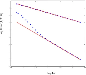
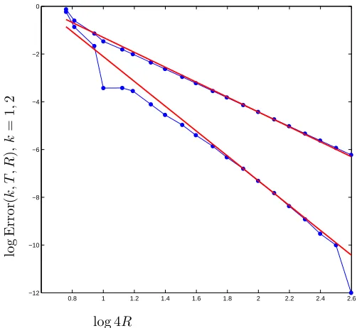
![Figure 6. Error in log scale for (4.35) in function of the number of cells per dimension[3 R ∈, 52] without zero-order term, with and without filtering: Slope −1 in both cases.](https://thumb-us.123doks.com/thumbv2/123dok_us/10074797.1993917/50.595.116.419.427.665/figure-error-scale-function-number-dimension-ltering-slope.webp)
![Figure 8. Error in log scale for (4.36) in function of the number of cells per dimensionof reference: SlopeR ∈ [3, 42] without zero-order term and without filtering, for the two different coefficients −1 and artificial super-linear convergence.](https://thumb-us.123doks.com/thumbv2/123dok_us/10074797.1993917/51.595.134.406.443.682/function-dimensionof-reference-ltering-dierent-coecients-articial-convergence.webp)