F. Coquel, M. Gutnic, P. Helluy, F. Lagouti`ere, C. Rohde, N. Seguin, Editors
A DIFFUSE INTERFACE MODEL FOR QUASI–INCOMPRESSIBLE FLOWS:
SHARP INTERFACE LIMITS AND NUMERICS
∗,∗∗,∗∗∗Gonca Aki
1, Johannes Daube
2, Wolfgang Dreyer
1, Jan Giesselmann
3, Mirko
Kr¨
ankel
2and Christiane Kraus
1Abstract. In this contribution, we investigate a diffuse interface model for quasi–incompressible flows. We determine corresponding sharp interface limits of two different scalings. The sharp interface limit is deduced by matched asymptotic expansions of the fields in powers of the interface. In particular, we study solutions of the derived system of inner equations and discuss the results within the general setting of jump conditions for sharp interface models. Furthermore, we treat, as a subproblem, the convective Cahn–Hilliard equation numerically by a Local Discontinuous Galerkin scheme.
1.
Introduction
We are interested in the modeling and numerical simulation of multiphase and multicomponent flows. We use a mixture approach, in which the constituents are either different substances or different phases of the same substance. In the description of multiphase and multicomponent flows, there are two different classes of models. Classically, one uses so called “sharp interface” models, where the interface between the substances or phases is described as a hypersurface. In the bulk domains separated by the interface, the fields – density and velocity – are subject to classical laws of fluid dynamics whereas at the interfacial surface the fields may be discontinuous and have to satisfy certain “jump conditions”, which enforce for instance conservation of mass and momentum. However, in many applications, these interfaces might become very hard to track numerically and their structure very hard to resolve. In particular, when surface tension is included in the model, sharp interface models collapse, in case the topology of the interface becomes singular, which happens when bubbles split or coalesce, cf. [17]. Therefore, phase field models have become an increasingly important tool for the numerical simulation in the last decade. In phase field models, some parameter indicates the distribution of the constituents. This parameter, as well as the fields, varies steeply but smoothly over some interfacial layer, which is thin, but has a nonzero thickness ε. The smoothing effect is achieved by considering energies, which
∗GA, WD and CK would like to thank the German Research Foundation (DFG) for financial support of the project ”Modeling and sharp interface limits of local and non-local generalized Navier–Stokes–Korteweg Systems”.
∗∗ JD and MK would like to thank the German Research Foundation (DFG) for financial support of the project within the research initiative ”Micro–Macro Modeling and Simulation of Liquid–Vapour Flows”.
∗∗∗JG would like to thank the German Research Foundation (DFG) for financial support of the project within the Cluster of Excellence in Simulation Technology (EXC 310/1) at the University of Stuttgart.
1
Weierstrass Institute for Applied Analysis and Stochastics, Berlin, Germany; e-mail:[email protected] & [email protected] & [email protected]
2
Department of Mathematics, University of Freiburg, Germany; e-mail:[email protected] & [email protected]
3
ACMAC, University of Crete, Greece; e-mail:[email protected]
c
EDP Sciences, SMAI 2012
depend on gradients of the fields, an idea going back to [24], which was already applied in [9]. For a review on phase field models in fluid mechanics, we refer to [6]. In the work at hand, we consider a model for a mixture of two incompressible fluids derived in [4]. Both fluids might be transformed into each other by a reaction or a phase transition.
Sharp interface models are physically well–founded and all jump conditions, but the kinetic relation, can be derived from classical conservation considerations. The notion of kinetic relation originates from the theory of solid–solid phase transitions [3], but it can also be applied to more general problems [19]. Phase field models, on the other hand, can be derived using entropy arguments, see [5] for a general framework. Nevertheless, they need to be verified. One important way to do this is to nondimensionalize the system and letting εgo to zero in order to identify physically meaningful sharp interface models.
The work at hand has two interests. The first one is determining the sharp interface limit of two different scalings. We will do this using the technique of formally matched asymptotic expansions, see [8]. Our second aim is to present a numerical scheme to solve an advective Cahn–Hilliard equation which is a subproblem of the whole model. We use a Local Discontinuous Galerkin (LDG) method based on theDuneframework. This type of method is known to handle the discretization of higher order derivatives easily and allows to implement higher order schemes, adaptivity and parallelization in a convenient way. In particular in case of convection dominated problems LDG schemes are superior to continuous Finite Element methods.
1.1.
Description of the Model
As pointed out before, the model under consideration is presented in [4], and a detailed derivation is given there. Thus, we will not give many details on the derivation. The model describes a mixture of two incom-pressible fluids having prescribed density ˜ρ1,ρ˜2,respectively. In case these densities coincide the model is fully
incompressible and the modeling goes back to [16], see also [14] for a thermodynamically consistent deriva-tion. Different generalizations to the generic case of fluids with different densities, i.e. ˜ρ16= ˜ρ2, can be found
in [1, 2, 7, 11, 20]. In this case, there is a certain amount of compressibility present in the model. This is due to the fact that the density depends on the mixture ratio of the two fluids.
Let us now give an account of the fields present in the model. By ϕ∈ Rwe denote the scaled amount of volume occupied by one of the constituents. We haveϕ= 1 in case only this constituent is present andϕ=−1 in case it is absent. Hence, the mass densities of the constituents ρ1, ρ2 are related to the total mass density
ρ=ρ(ϕ) via
ρ=ρ1+ρ2= ˜ρ1
1 +ϕ
2 + ˜ρ2 1−ϕ
2 . (1)
Furthermore,v∈Rd is the mass averaged fluid velocity satisfying
ρv=ρ1v1+ρ2v2, (2)
wherev1,v2are the velocities of the constituents. In addition, the pressurep=p(ϕ) is given via a constitutive
relation as a function ofϕsuch that
p(ϕ) =ϕW′(ϕ)−W(ϕ), (3)
whereW =W(ϕ) is the Helmholtz free energy density. We want to state for later use that (3) implies
p′(ϕ) =ϕW′′(ϕ). (4)
We impose that the Helmholtz free energy density has a special double–well shape. In particular, we assume
W(ϕ)>0 ∀ϕ∈R\ {−1,1}, and W(−1) =W(1) = 0 (5)
and that there existα1, α2∈(−1,1) such that
In this way, the Maxwell points ofW, which are defined as the valuesϕ1< ϕ2 satisfying
W′(ϕ1) =W′(ϕ2) =W(ϕ
2)
−W(ϕ1)
ϕ2−ϕ1 , (7)
are given byϕ1 =−1, ϕ2 = 1. We like to point out that because of (4) the nonconvex Helmholtz free energy density implies a nonmonotone pressure function.
The remaining parameters of the model are given as follows: mJ and mr are the diffusion and reaction
mobility, respectively, γ denotes the capillarity coefficient and c+, c− are related to the densities ˜ρ1,˜ρ2 with
˜
ρ1<ρ˜2 as follows
c+= 1
˜
ρ1 +
1 ˜
ρ2
, c−= 1 ˜
ρ1 −
1 ˜
ρ2
. (8)
In addition, let Ω⊂Rdbe a domain with smooth boundary and [0, T) the time interval of interest. The system, cf. [4], reads in [0, T)×Ω:
ϕt+ div(ϕv) =c+(mJ∆−mr)(c+µ+c−λ), (9)
ρ(ϕ)(vt+ (v· ∇)v) +∇(p(ϕ) +λ) = div(σN S) +γϕ∇∆ϕ, (10)
div(v) =c−(mJ∆−mr)(c+µ+c−λ), (11)
where
µ:=W′(ϕ)−γ∆ϕ, p(ϕ) =ϕW′(ϕ)−W(ϕ), σN S :=η(ϕ) div(v)I+ ˆη(ϕ)(∇v+ (∇v)T). (12)
The evolution of the model is described by (ϕ,v, λ), where λ ∈ R presents a Lagrange multiplier, which ensures the incompressibility of the pure constituents. In particular, µ is the chemical potential, σN S is the
Navier–Stokes tensor, and η and ˆη denote the bulk and shear viscosity, respectively, which are interpolated between the two pure constituents. They satisfy η(ϕ) + 2ˆη(ϕ)≥0 and ˆη(ϕ)>0 for allϕ∈[−1,1].
It is important to note that we have to deal with a rather complicated divergence constraint for the velocity. This is in contrast to the model introduced in [2], where a volume averaged velocity is considered.
To avoid physically meaningless scalings, it is important to nondimensionalize the system before introducing the scaling.
1.2.
Nondimensionalization
In order to nondimensionalize the system (9)-(12), we introduce the reference quantities ¯x, ¯t, ¯v, ¯p, ¯λ, ¯c+, ¯c−,
¯
η, ¯γ, ¯mJ, ¯mr, ¯ρsuch that
x= ¯xx∗, t= ¯tt∗, v= ¯vv∗, p= ¯pp∗, λ= ¯λλ∗, ρ= ¯ρρ∗, c+= ¯c+c∗+, c−= ¯c−c∗−, η = ¯ηη∗, ηˆ= ¯ηηˆ∗,
γ= ¯γγ∗, mJ = ¯mJm∗J, mr= ¯mrm∗r, µ= ¯pµ∗, W = ¯pW∗.
Note that ϕ is a scaled phase field variable interpolating the density between ˜ρ1 and ˜ρ2, see (1). Hence, it
is already dimensionless. Only for reasons of consistent notation, we will use the symbol ϕ∗ instead of ϕ in
the nondimensionalized system. Moreover, we remark that the choicesp= ¯pp∗, µ= ¯pµ∗, andW = ¯pW∗ are
nondimensionalized version of the system (9)-(11):
1 ¯
t∂t∗ϕ
∗+v¯
¯
xdiv
∗(ϕ∗v∗)−¯c
+c∗+
m¯J ¯
x2 m∗J∆∗−m¯rm∗r
¯
c+pc¯∗+µ∗+ ¯c−λc¯ ∗−λ∗
= 0, (13)
¯
ρρ∗(ϕ∗)
¯
v
¯
t∂t∗v
∗+¯v2
¯
x(v
∗· ∇∗)v∗
+ 1
¯
x∇
∗(¯pp∗(ϕ∗) + ¯λλ∗)−η¯v¯
¯
x2div
∗(σ∗ N S)−
¯
γ
¯
x3γ
∗ϕ∗∇∗∆∗ϕ∗= 0, (14)
¯
v
¯
xdiv
∗(v∗)−c¯ −c∗−
m¯J ¯
x2 m∗J∆∗−m¯rm∗r
¯
c+pc¯∗+µ∗+ ¯c−λc¯ ∗−λ∗
= 0. (15)
For the constitutive laws, we clearly havep= ¯pp∗ and obtain
σ∗
N S:=η∗(ϕ∗) div∗(v∗)I+ ˆη∗(ϕ∗)(∇∗v∗+ (∇∗v∗)T), pµ¯ ∗= ¯p(W∗)′(ϕ∗) +
¯
γ
¯
x2γ∗∆∗ϕ∗. (16)
We denote by M the Mach number and by Re the Reynolds number, which are given by M = ¯vqρp¯¯, and Re = ρ¯¯vη¯x¯, respectively. By the definitions ofc+ andc−, see (8), it is reasonable to choose ¯c+=ρ1¯and ¯c−= qρ¯¯,
where ¯qis an additional reference quantity, that measures the difference between the densities ˜ρ1and ˜ρ2in the
following sense
¯
q=ρ˜2−ρ˜1 ˜
ρ1ρ˜2
¯
ρ= ρˆ2−ρˆ1 ˆ
ρ1ρˆ2
, where ρˆi= ˜
ρi
¯
ρ for i= 1,2. (17)
For the reference velocity ¯v, we make the choice ¯v= x¯ ¯
t, although other physically reasonable scalings, like e.g.
¯
v=qpρ¯¯, exist. Our choice ensures that∂t∗ϕ∗ and div∗(ϕ∗v∗) appear in the same order. Therefore, we get
∂t∗ϕ∗+ div∗(ϕ∗v∗)−
¯
tp¯ ¯
ρ2c∗+
m¯J ¯
x2 m∗J∆∗−m¯rm∗r c∗+µ∗+ ¯qc∗−
¯ λ ¯ pλ ∗
= 0, (18)
ρ∗(ϕ∗) (∂t∗v∗+ (v∗· ∇∗)v∗) +
1 M2∇
∗
p∗(ϕ∗) +λ¯ ¯
pλ
∗
−Re1 div∗(σ∗N S)− γ¯
M2x¯2p¯γ
∗ϕ∗∇∗∆∗ϕ∗= 0, (19)
div∗(v∗)−¯tp¯q¯ ¯
ρ2c
∗ −
m¯J ¯
x2 m
∗
J∆∗−m¯rmr∗ c∗+µ∗+ ¯qc∗−
¯ λ ¯ pλ ∗
= 0, (20)
and
µ∗= (W∗)′(ϕ∗) + γ¯
¯
x2p¯γ∗∆∗ϕ∗. (21)
We introduce a small parameterε >0, representing the width of the interface, such that
ε= r
¯
γ
¯
x2p¯. (22)
This is justified by the following remark.
Remark 1.1 (Interfacial thickness). The fact thatε, see (22), represents the thickness of the interface may be justified by constructing recovery sequences for the Γ–limit of the energy functional
Z
Ω
1
√¯γW(ϕ) +√γ¯|∇ϕ|2dx as√¯γ→0,
In addition to (22), we choose the following scalings
¯
q= 1, t¯p¯m¯J
¯
ρ2x¯2 =
1
ε, m¯r= 0, and
¯
λ
¯
p = 1. (23)
Finally, inserting the scalings (22) and (23) into the system (18)-(21) leads to
∂t∗ϕ∗+ div∗(ϕ∗v∗) =
1
εc
∗
+m∗J∆∗ c+∗µ∗+c∗−λ∗
, (24)
ρ∗(ϕ∗) (∂t∗v∗+ (v∗· ∇∗)v∗) +
1 M2∇
∗(p∗(ϕ∗) +λ∗) = 1
Rediv
∗(σ∗ N S) +
ε2
M2γ
∗ϕ∗∇∗∆∗ϕ∗, (25)
div∗(v∗) = 1
εc
∗
−m∗J∆∗ c+∗µ∗+c∗−λ∗
. (26)
We only give the constitutive equation forµas it is the only one containingε:
µ∗= (W∗)′(ϕ∗)−ε2γ∗∆∗ϕ∗. (27)
In this paper, for the remaining quantities, we will study the following two scalings
Re = 1, and M =ε, (28)
Re = 1
ε, and M =
√
ε, (29)
which we callstrong capillarity regime, andlow viscosity regime, respectively. For these scalings, we will study the comportment of solutions of the system (24)-(27), when the parameter ε tends to 0. This will be carried out by the technique of matched asymptotic expansions in section 5. For convenience, we will omit the symbol ∗ in the sequel. Note that in the context of Navier–Stokes–Korteweg systems, the zero Mach number
limit has been considered in [15].
1.3.
Results
The paper is organized as follows. We first show that the model dissipates energy, see section 2. Section 3 describes a general framework of sharp interface models. Then, we recall several results and definitions from the theory of matched asymptotic expansions in section 4. In the main part, section 5, we determine the sharp interface limits of the two different scalings in (28) and (29). In subsection 5.1, we present a scaling where the capillarity effects are so strong that the mean curvature of the phase boundary has to be constant, while in the second scaling, see subsection 5.2, the Navier–Stokes tensor vanishes in the limit. Finally, we present a numerical treatment of a part of the model in section 6. We have implemented a Local Discontinuous Galerkin scheme for the Cahn–Hilliard equation with a convection term, which governs the evolution of the phase field variable. We show that the scheme has the expected order of approximation in the one–dimensional case. We give two examples in two dimensions to demonstrate the expected behavior in the case with and without an additional advection term.
2.
Entropy Inequality
phase to the other. In addition, the entropy inequality can be seen as a first (small) step to establish stability of the model. As the energy dissipation of the model does not depend on the scaling, we consider (9)-(12) instead of any scaled version. In particular, our discussion includes the casemr6= 0.
We start by providing some properties of smooth solutions of the system (9)-(12) for later use.
Remark 2.1. Let (ϕ,v, λ) be a smooth solution of the system (9)-(12). (1) By combining (9) and (11), we find
ϕt+ div(ϕv) =c+mJ∆(c+µ+c−λ)−c+mr(c+µ+c−λ) =
c+
c−div(v). (30)
(2) From (1), (8), and (30) follows, that mass conservation is valid, i.e.
ρ(ϕ)t+ div(ρ(ϕ)v) = 0. (31)
To see that the system (9)-(12) is physically meaningful, we have to check that its solutions satisfy the balance of momentum for an appropriate stress tensor.
Remark 2.2. In [13], a thermodynamically consistent Korteweg stress tensor σK with temperature is
intro-duced which reduces for isothermal processes to σK = γ(ϕ∆ϕ+ 1 2|∇ϕ|
2
)I−γ∇ϕ⊗ ∇ϕ. Since div(σK) =
γϕ∇∆ϕ, for this choice the balance of momentum reads
(ρ(ϕ)v)t+ div(ρ(ϕ)v⊗v) +∇(p(ϕ) +λ) = div(σN S) + div(σK) = div(σN S) +γϕ∇∆ϕ, (32)
which, in view of (31), is equation (10).
Theorem 2.3. Let Ω⊂Rd be a domain with smooth boundary and(ϕ,v, λ)be a smooth solution of the system
(9)-(12)satisfying the boundary conditions
∇ϕ·ν= 0, v=0, and ∇(c+µ+c−λ)·ν= 0 (33)
on [0, T)×∂Ω. Then, the total energy is nonincreasing, i.e.
d dt
Z
Ω
W(ϕ) +12γ|∇ϕ|2+12ρ(ϕ)|v|2dx
=−
Z
Ω
mJ|∇(c+µ+c−λ)|2+mr(c+µ+c−λ)2+σN S:∇vdx≤0. (34)
Proof. The energy density e = e(ϕ,∇ϕ,v) := W(ϕ) + 1 2γ|∇ϕ|
2
+ 1
2ρ(ϕ)|v| 2
possesses the time derivative
et=W′(ϕ)ϕt+γ∇ϕ· ∇ϕt+v·(ρ(ϕ)v)t−12|v|2ρ(ϕ)t. If we replace all time derivatives with the help of (30),
(31), and (32), we get
et=W′(ϕ)
c+
c−div(v)−div(ϕv)
+γ∇ϕ· ∇c+
c−div(v)−div(ϕv)
+v·(div(σN S) + div(σK))
−v· ∇(p(ϕ) +λ)−1 2div
ρ|v|2v.
AbbreviatingA:=et+ div(ev) + div((p(ϕ)I−σN S−σK)v) yields
A=W′(ϕ)c+
c−div(v)−div(ϕv)
+γ∇ϕ· ∇c+
c−div(v)−div(ϕv)
−σN S :∇v−σK:∇v
−v· ∇λ+ (p(ϕ) +W(ϕ)) div(v) +∇W(ϕ)·v+1
2γdiv(|∇ϕ|
After some rearrangements, using (3), this reduces to
A= c+
c−W
′(ϕ) div(v) + c+
c−γ∇ϕ· ∇div(v)−
σN S :∇v−v· ∇λ−γdiv(div(v)ϕ∇ϕ).
Now, we integrate overA. Making use of the boundary conditions (33) and recalling (12) and (30), we obtain
d dt
Z
Ω
edx
=
Z
Ω
hc +
c−(W
′(ϕ)−γ∆ϕ) +λidiv(v)−σ
N S:∇vdx
=−
Z
Ω
mJ|∇(c+µ+c−λ)|2+mr(c+µ+c−λ)2+σN S :∇vdx.
3.
Sharp Interface Setting
This section is devoted to describe a general framework for sharp interface models, into which the sharp interface limits derived in section 5 have to fit.
For notational simplicity, we consider the two–dimensional case. We are convinced that our sharp interface limits already discover all information on the bulk equations and jump conditions in this case and the notational burden of considerations in higher dimensions would not be justified.
We consider a C2–hypersurface Γ(t), t
∈ [0, T). Any point of Γ(t) is given by the function r(t, s), where
s∈I⊂R,Ibounded interval, is used to parametrize Γ(t),i. e. r: [0, T)×I→R2. A two–phase body Ω⊂R2 is decomposed by theinterfaceΓ(t) into two bulk phases Ω+(t) and Ω−(t), i.e. we have Ω = Ω+(t)
∪Ω−(t)∪Γ(t),
t∈[0, T).
We assign to Ω a generic additive quantity Ψ(t), which is represented by
Ψ(t) = Z
Ω+(t)
ψ(t,x) dx+ Z
Ω−(t)
ψ(t,x) dx+ Z
I
ψΓ(t, s) ds,
where ψ andψΓ are the corresponding densities of Ψ. The quantityψ may change due to fluxes and sources.
This is locally described by equations of balance for the densities. In Ω±(t), the equations of balance read
∂ψ
∂t + div(ψv+f) =ξ,
where v : [0, T)×Ω± → R2 is the fluid velocity, f : [0, T)
×Ω± → R2 denotes a nonconvective flux and
ξ: [0, T)×Ω±→Ris a source density. On the interface Γ(t), we have
−wν[[ψ]] + [[ψv+f]]·ν=−∂ψΓ
∂t −ψΓ(divΓ(wtt)−κwν)−divΓ(fΓ) +ξΓ. (35)
The newly introduced quantities are the interface normal ν : [0, T)×I → R2, the interface velocity w :
[0, T)×I→R2, which is decomposed into normal and tangential components, i. e. wν and wt (see (39)), the
interface flux fΓ : [0, T)×I→R2 and the interface sourceξΓ: [0, T)×I→R. Double brackets [[·]] denote the
difference of a bulk quantity at the left and right side of the interface and divΓ is the surface divergence.
4.
Asymptotic Analysis
4.1.
Decomposition of the Domain
We decompose the given physical domain Ω ⊂ R2 into two bulk regions Ω+(t;ε) and Ω−(t;ε), which are
separated by an interfacial surface Γ(t;ε), ε > 0 small. The interface Γ(t;ε) is assumed to be a smoothly evolving C1([0, T),C2(Ω))–hypersurface which is defined by
Γ(t, ε) :={x∈Ω :ϕε(t,x) = 0},
whereϕε is the solution of (24)-(27). The bulk domains are given by
Ω−(t, ε) :={x∈Ω : ϕε(t,x)<0} and Ω+(t, ε) :={x∈Ω : ϕε(t,x)>0}.
We assume that a limiting curve Γ = Γ(t) exists whenε tends to zero. The corresponding bulk domains are abbreviated by Ω−(t) and Ω+(t).
In the sequel, we will consider the so called outer setting in the bulk domains and the so called inner setting in a neighborhood of Γ(t).
4.2.
Outer Setting
Another main assumption of formally matched asymptotics is that all quantities have asymptotic expansions in the small parameterε, which is related to the thickness of the interfacial layer, cf. Remark 1.1 for details. We assume the existence of the following expansions for the velocity v, the phase field parameter ϕand the Lagrange multiplierλin the bulk domains Ω±(t, ε):
v(t,x;ε) =v0(t,x) +εv1(t,x) +o(ε), (36)
ϕ(t,x;ε) =ϕ0(t,x) +εϕ1(t,x) +ε2ϕ2(t,x) +o(ε2), (37)
λ(t,x;ε) =λ0(t,x) +ελ1(t,x) +ε2λ2(t,x) +o(ε2). (38)
These expansions will be inserted in the scaled equations to obtain the equations satisfied by outer solutions, cf. e.g. Definition 5.1.
4.3.
Inner Setting
The position of the limiting phase boundary Γ(t) is given as a functionr(t, s),whereI⊂Ris some bounded interval which we use as parameter domain ands∈Iis used to parameterize the interface. From the mapr, we can compute tangent and normal vectors to the interface as well as the interface velocity. The tangent vector pointing in counterclockwise direction and the unit normal to the interface pointing to the left of the curve are given by
t(t, s) =
∂r1 ∂s(t, s),
∂r2 ∂s(t, s)
T
, and ν(t, s) = 1
|t(t, s)|
−∂r 2
∂s(t, s), ∂r1
∂s(t, s) T
,
respectively, wherer1, r2 denote the components ofrin Cartesian coordinates. In the following, we abbreviate the partial derivative of a quantityl with respect tosbyls. The mean curvatureκis defined by
κ= r
1
sr2ss−r1ssrs2
((r1
s)2+ (r2s)2)
The interface velocity, which is defined as the time derivative of r, can be decomposed into tangential and normal components by
w= ∂r
∂t =wtt+wνν. (39)
There are some identities linking s–derivatives oftandν withκ:
tj
|t|
s
=κ|t|νj and (νj)s=−tjκ forj= 1,2.
To each t∈[0, T), there exists some neighborhood N(t)⊂Ω of Γ(t) such that every point (x1, x2)∈ N(t)
can be represented as
x1 x2
(τ, s, z) =r(τ, s) +εzν(τ, s), τ=t. (40)
Thus,zis the scaled distance from the interface in normal direction. The small parameterεis introduced here to zoom into the interfacial region. We use (40) to change variables from (t, x1, x2) to (τ, s, z). For a scalar or a
Cartesian component of a vectorψ,which is defined in inner and outer coordinates, i.e. ψ(t, x1, x2) = Ψ(τ, s, z),
the partial derivatives transform as follows:
∂ψ ∂x1 ∂ψ ∂x2 ∂ψ ∂t =
(1 +εzκ)|t1|2t1 ε−1ν1 0
(1 +εzκ) 1
|t|2t
2 ε−1ν2 0
−(1 +εzκ)(wt+εz|t1|2t
i(νi)
τ) −ε−1wν 1
∂Ψ ∂s ∂Ψ ∂z ∂Ψ ∂τ
+O(ε2), (41)
for a fixed point (τ, s, z). The derivation of (41) can be found in e.g. [12]. In accordance with (36)-(38), we assume that the quantities in inner variables can also be expanded in ε:
V(τ, s, z;ε) =V0(τ, s, z) +εV1(τ, s, z) +o(ε), (42)
Φ(τ, s, z;ε) = Φ0(τ, s, z) +εΦ1(τ, s, z) +ε2Φ2(τ, s, z) +o(ε2), (43)
Λ(τ, s, z;ε) = Λ0(τ, s, z) +εΛ1(τ, s, z) +ε2Λ2(τ, s, z) +o(ε2). (44)
By using (41) and plugging (42)-(44) into the scaled systems, we obtain the equations satisfied by the inner solutions, cf. e.g. (65)-(70) and Definition 5.2, by comparing coefficients of different powers ofε.
4.4.
Matching Conditions
Inner and outer quantities are matched by the usual procedure, see [8,12] for details. However, for convenience of the reader, we recall the matching conditions, one obtains up to second order. Note that we use Einstein summation convention:
Ψ0(τ, s, z)→ψ0±(τ,r(τ, s)) z→ ±∞, (45)
Ψ1(τ, s, z)−
∂ψ0
∂xj
±
(τ,r(τ, s))νj(τ, s)z→ψ1±(τ,r(τ, s)) z→ ±∞, (46)
Ψ2(τ, s, z)−
1 2z
2
∂2ψ0
∂xi∂xj
±
(τ,r(τ, s))νiνj−z
∂ψ1
∂xi
±
We also get conditions for the derivatives which are basically derived by differentiating the equations leading to the above conditions.
Ψ0,τ →
∂ψ0
∂xj
±
(τ,r(τ, s))wj(τ, s) +
∂ψ0
∂t ±
(τ,r(τ, s)) z→ ±∞, (48)
Ψ0,s→
∂ψ0
∂xj
±
(τ,r(τ, s))tj(τ, s) z→ ±∞, (49)
Ψ1,z→
∂ψ0
∂xj
±
(τ,r(τ, s))νj(τ, s) z→ ±∞, (50)
Ψ0,z,Ψ0,zz,Ψ1,zz→ 0 z→ ±∞, (51)
Ψ2,z−z
∂2ψ
0
∂xi∂xj
±
(τ,r(τ, s))νiνj→
∂ψ1
∂xi
±
(τ,r(τ, s))νi(τ, s) z→ ±∞, (52)
Ψ2,zz→
∂2ψ0
∂xi∂xj
±
(τ,r(τ, s))νi(τ, s)νj(τ, s) z→ ±∞. (53) We impose that all these limits are attained superlinearly fast.
5.
Derivation of the Sharp Interface Limits
In (28) and (29), we have suggested two scalings of the system (24)-(27). In this section, we will explore the sharp interface limits for these scalings.
5.1.
Strong Capillarity Scaling
In this section, we will consider a scaling with extremely strong capillary effects. We will see that the sharp interface limit problem is given by the incompressible Navier–Stokes equations, subject to a Young–Laplace condition for the jump of a lower order pressure than the one present in the momentum balance. The extremely strong capillary effects enforce interfaces of constant mean curvature. The scaled system corresponds to very small Mach numbers, i.e. M∼ε, and high mobilities and reads
ϕt+ div(ϕv) =
1
εc+mJ∆(c+µ+c−λ), (54)
ρ(ϕ)(vt+ (v· ∇)v) +
1
ε2∇(p(ϕ) +λ) = div(σN S) +γϕ∇∆ϕ, (55)
div(v) =1
εc−mJ∆(c+µ+c−λ), (56)
with the constitutive laws
µ=W′(ϕ)−γε2∆ϕ, p(ϕ) =ϕW′(ϕ)−W(ϕ), σN S =η(ϕ) div(v)I+ ˆη(ϕ)(∇v+ (∇v)T). (57)
The equations for (λ0,v0, ϕ0, λ1, ϕ1) in the bulk phases are obtained, by plugging expansions (36)-(38) into
(54)-(56) and by gathering terms having the same order inε. Hence, we have in orderε−2
0 =∇(p(ϕ0) +λ0), (58)
in orderε−1
0 = ∆(c+µ0+c−λ0), (59)
and in orderε0
ϕ0,t+ div(ϕ0v0) =c+mJ∆(c+µ1+c−λ1), (61)
div(v0) =c−mJ∆(c+µ1+c−λ1). (62)
In addition, we find by using the expansions in (57)
µ0:=W′(ϕ0), µ1:=W′′(ϕ0)ϕ1, p0=p(ϕ0), p1=p′(ϕ0)ϕ1. (63)
We want to stress that (57) are definitions, in contrast to equations (54)-(56). Thus, we cannot prescribe an expansion forµ,but the expansion ofµis prescribed by (57) and the expansion ofϕ.These equations motivate the following definition.
Definition 5.1 (Outer solution). A tuple (λ0,v0, ϕ0, λ1, ϕ1) such that
λ0, ϕ1, λ1∈C0([0, T),C2( ¯Ω±(t),R)),
ϕ0∈C1([0, T),C0( ¯Ω±(t),R))∩C0([0, T),C2( ¯Ω±(t),R)),
v0∈C0([0, T),C1( ¯Ω±(t),R2)),
is called anouter solution of the strong capillarity regimeprovided it satisfies (58)-(62), whereµ0, µ1are
given by (63), andϕ06≡cc+
−. In addition, the boundary condition
∇ϕ0·ν= 0 on [0, T)×∂Ω (64)
has to be satisfied.
The inner equations are obtained as follows: We perform the coordinate transformation given by (40) in (54)-(56). Then, we plug in the expansions in inner coordinates (42)-(44). Finally, we gather terms of the same order ofε,which yields
(c+M0+c−Λ0)zz=0, (65)
(p(Φ0) + Λ0)z=γΦ0Φ0,zzz, (66)
(c+M1+c−Λ1)zz−κ(c+M0+c−Λ0)z=0, (67)
(p(Φ0)Φ1+ Λ1)zν+ (p(Φ0) + Λ0)s
t
ktk2 =((η(Φ0) + 2ˆη(Φ0))V0,z·ν)zν+ (ˆη(Φ0)V0,z· t
ktk2)zt (68)
+γ(Φ1Φ0,zzz+ Φ0Φ1,zzz−κΦ0Φ0,zz)ν+γΦ0Φ0,zzs t
ktk2, −wνΦ0,z+ (Φ0V0·ν)z=c+mJ(c+M2+c−Λ2)zz−κ(c+M1+c−Λ1)z (69)
+ (c+M0+c−Λ0)ss−zκ2(c+M0+c−Λ0)z,
c+
c−(V0·ν)z=c+mJ
(c+M2+c−Λ2)zz−κ(c+M1+c−Λ1)z (70)
+ (c+M0+c−Λ0)ss−zκ2(c+M0+c−Λ0)z
.
Furthermore, doing the same for (57) gives
P0=p(Φ0), P1=p′(Φ0)Φ1,
M0=W′(Φ0)−γΦ0,zz, M1=W′′(Φ0)Φ1−γΦ1,zz+γκΦ0,z,
M2=W′′(Φ0)Φ2+
1 2W
′′′(Φ
0)Φ21−γΦ2,zz+γκΦ1,z−γΦ0,ss−γzκ2Φ0,z.
This motivates the following definition of inner solutions.
Definition 5.2 (Inner solution and matching solution). A tuple (Λ0,V0,Φ0,Λ1,Φ1,Λ2,Φ2) such that
Λ0∈C0([0, T),C0(I,C2(R)))∩C0([0, T),C2(I,C0(R))),
Λ1,Λ2∈C0([0, T)×I,C2(R)),
Φ0∈C0([0, T)×I,C4(R))∩C0([0, T),C2(I,C2(R)))
Φ1,Φ2∈C0([0, T)×I,C4(R)),
V0∈C0([0, T)×I,C2(R,R2)),
is called an inner solution of the strong capillarity regime, provided it satisfies (65)-(70) and Φ0 6≡ cc+
−,
whereP0, P1, M0, M1andM2 are given by (71).
A tuple (λ0,v0, ϕ0, λ1, ϕ1,Λ0,V0,Φ0,Λ1,Φ1,Λ2,Φ2) is called a matching solution of the strong cap-illarity regime, if (λ0,v0, ϕ0, λ1, ϕ1) is an inner and (Λ0,V0,Φ0,Λ1,Φ1,Λ2,Φ2) is an outer solution of the
strong capillarity regime and both are linked by the matching conditions (45)-(53).
Theorem 5.3. Let(λ0,v0, ϕ0, λ1, ϕ1,Λ0,V0,Φ0,Λ1,Φ1,Λ2,Φ2)be a matching solution of the strong capillarity
regime. Then, ϕ0= 1in Ω+(t) for allt ∈[0, T) andϕ0=−1 inΩ−(t) for all t∈[0, T), while λ0 is constant
in space in the whole domain. Moreover, in the bulk domainsΩ±(t) the fields satisfy
div(v0) = 0, ∆(c+W′′(ϕ0)ϕ1+c−λ1) = 0, ∇(p′(ϕ0)ϕ1+λ1) = 0. (72)
At the interface Γthey are subject to the following jump conditions
[[v0·t]] = 0, [[c+W′′(ϕ0)ϕ1+c−λ1]] = 0, [[v0·ν]] =c−mJ[[∇(c+W′′(ϕ0)ϕ1+c−λ1)]]·ν, (73)
[[W′′(ϕ0)ϕ1]] =
Z ∞
−∞
((η(Φ0) + 2ˆη(Φ0))(V0·ν)z)z
Φ0−cc+
−
dz, [[p′(ϕ0)ϕ1+λ1]] =κ
Z ∞
−∞
(Φ0,z)2dz, (74)
and the normal velocity of the interface is given by
wν=hv0·νi −c+mJ
2 [[∇(c+W
′′(ϕ
0)ϕ1+c−λ1)]]·ν, (75)
wherehv0·νidenotes the mean value 1 2(v
+
·ν+v−·ν). Furthermore, the mean curvature of the interface has
to be constant with respect to the interface parameter s.
Remark 5.4. Let us also consider the momentum equation of orderε−1. Abbreviatingp′(ϕ0)ϕ2 +12p′′(ϕ0)ϕ21,
byp2, we obtain from the outer expansions and the fact thatϕ0is constant the equation:
ρ(ϕ0)(v0,t+ (v0· ∇)v0) +∇(p2+λ2) = div((σN S)0) in [0, T)×Ω±(t). (76)
Here, (σN S)0denotes the leading order ofσN S,where we have substitutedϕ,vbyϕ0,v0.Thus, one has to solve
incompressible Navier–Stokes equations in the bulk, where (p2+λ2) takes the role of the pressure. However,
one cannot get the classical Young–Laplace law, as the surface tension is so strong in this case that it enforces the Young–Laplace law forp1+λ1.If one considers the appropriate inner equations, one obtains – after rather
cumbersome calculations –
[[ρ(ϕ0)(v0·ν−wν)2+p2+λ2−σij
N Sνiνj]] =−2κ
Z ∞
−∞
ˆ
η(Φ0)V0,z·νdz+ 2γκ
Z ∞
−∞
Φ0,zΦ1,zdz
−γCss
Z ∞
−∞
(Φ0,z)2dz+γκ2C
Z ∞
−∞
Here, C is a function, depending on τ and s, which appears as a translation term in the argument of Φ0
compared with the reference solution ¯Φ0 satisfying ¯Φ0(0) = 0, cf. (102).
Proof of Theorem 5.3. As the proof is quite long, we decompose it into several parts.
Part 1: Firstly, we prove that ϕ0 = 1 in Ω+(t) for all t ∈ [0, T) and ϕ0 = −1 in Ω−(t) for all t ∈ [0, T).
Secondly, we verify thatλ0 is constant in space in the whole domain.
We start by dividing (65) byc− and subtracting (66), which gives because of (4) and (51)
c+
c−W
′′(Φ
0)Φ0,z−Φ0W′′(Φ0)Φ0,z =γ
c+
c−Φ0,zzz−γΦ0Φ0,zzz. (78)
For Φ06=cc+−, it follows
W′′(Φ0)Φ0,z =γΦ0,zzz. (79)
Now, since Φ0 ∈C0([0, T)×I, C3(R)), we may conclude by a continuity argument that (79) is equivalent to
(78). This implies, using (45),
[[W′(ϕ0)]] = 0. (80)
Integrating (79) and multiplying it by Φ0,z, we obtain
W′(Φ0)Φ0,z=γΦ0,zΦ0,zz+W′(ϕ±0)Φ0,z
=⇒[[W(ϕ0)]] =
1 2
Z ∞
−∞
((Φ0,z)2)zdz
| {z }
=0
+W′(ϕ±0)[[ϕ0]]. (81)
From (81) we learn that ϕ±0 are the Maxwell points of W, cf. (7) for the definition. Due to our choice of W,
this means
ϕ±0 =±1. (82)
We know from (58) thatp(ϕ0) +λ0is constant in the bulk phases. Furthermore, we get from (66)
[[p(ϕ0) +λ0]] =
Z ∞
−∞
Φ0Φ0,zz−
1 2Φ
2 0,z
z
dz= 0. (83)
Hence, there is some time dependent functionK=K(t), such that
p(ϕ0) +λ0=K(t) (84)
in the bulk phases. Moreover, we know by integrating (65) that
[[c+W′(ϕ0) +c−λ0]] = 0. (85)
Because of (58), (59), (64) and (82) the function f0:=c+W′(ϕ0)−c−p(ϕ0) satisfies the following problem in
Ω+(t) (and a similar problem in Ω−(t)):
∆f0= 0 in Ω+(t), ∇f0·ν= 0 on∂Ω∩Ω+(t), f0= 0 on Γ. (86)
Problem (86) is uniquely solvable and the obvious solution is
Due to the assumption (3) on the double well potential, this yields
ϕ0=±1 in Ω±(t). (88)
Finally, we combine (84) and (88) to see thatλ0 is constant in space in the whole domain.
Part 2: We show that div(v0) = 0 and ∆(c+W′′(ϕ0)ϕ1+c−λ1) = 0 hold in the bulk phases Ω±(t). Then,
we prove the jump condition [[c+W′′(ϕ0)ϕ1+c−λ1]] = 0 on Γ(t).
Combining (61) and (62), we get
ϕ0,t+∇ϕ0·v0+ϕ0div(v0) =
c+
c− div(v0). (89)
In view of (88), this means
c+
c− −ϕ0
| {z }
>0
div(v0) = 0 =⇒div(v0) = 0. (90)
Furthermore,by plugging (90) into (62), we find
∆(c+W′′(ϕ0)ϕ1+c−λ1) = 0. (91)
We continue by considering the inner equations. By (50) and (65) equation (67) becomes
(c+M1+c−Λ1)zz= 0.
This implies, using the matching condition (50),∇ϕ0= 0 and∇λ0= 0
(c+M1+c−Λ1)z= (∇(c+W′(ϕ0) +c−λ0))±·ν= 0. (92)
Thus, because of (46), we get
c+M1+c−Λ1=c+W′′(ϕ±0)ϕ±1 +c−λ±1, (93)
which directly implies
[[c+W′′(ϕ0)ϕ1+c−λ1]] = 0. (94)
Part 3: We show the jump conditions [[v0·t]] = 0 and [[p′(ϕ0)ϕ1+λ1]] =κR−∞∞ (Φ0,z)2dzon Γ(t). Furthermore,
we conclude that the mean curvatureκis constant in space.
Due to (60), we find numbersK±(t), only depending on time, such that
p′(ϕ0)ϕ1+λ1=K±(t) in Ω±(t). (95)
Now, let us consider (68) to determine the jump of the first order expression for the pressure plus the Lagrange multiplier, i. e. p′(ϕ0)ϕ1+λ1, at the interface. Decomposing (68) into normal and tangential part, we obtain
(p′(Φ0)Φ1+ Λ1)z = (¯η(Φ0)(V0·ν)z)z+γ(Φ1Φ0,zzz+ Φ0Φ1,zzz−κΦ0Φ0,zz), (96)
(p(Φ0) + Λ0)s= (ˆη(Φ0)(V0· t
ktk2)z)zktk 2+
γΦ0Φ0,zzs, (97)
where we abbreviate ¯η(Φ0) =η(Φ0) + 2ˆη(Φ0).Let us first deal with (97). We already know from (66)
p(Φ0) + Λ0=γΦ0Φ0,zz−
γ
2(Φ0,z)
2+
wherep(ϕ±0) +λ±0 is independent ofs. Plugging (66) into (97), we find
γ
Φ0Φ0,zz−
1 2(Φ0,z)
2
s
= (ˆη(Φ0)(V0· t
ktk2)z)zktk 2+γΦ
0Φ0,zzs, (99)
which, in turn, implies
γΦ0,sΦ0,zz−γΦ0,zΦ0,sz= (ˆη(Φ0)(V0· t
ktk2)z)zktk 2
. (100)
To understand the implications of (100), we have to investigate the s dependency of Φ0 more carefully. We
know that Φ0 satisfies
W′(Φ0) =γΦ0,zz+W′(±1) =γΦ0,zz, Φ0(±∞) =±1. (101)
As only the boundary data of Φ0 and Φ0,z are prescribed at infinity this does not determine Φ0 uniquely, but
we can write each solution as
Φ0(τ, s, z) = ¯Φ0(z+C(τ, s)) (102)
where ¯Φ0 is the unique solution of (101) satisfying ¯Φ0(0) = 0 andC is a translational constant with respect to
z.We like to mention that ¯Φ0is a function of only one variable. Equation (102) has the following consequences
for the partial derivatives of Φ0:
Φ0,z(τ, s, z) = ¯Φ′0(z+C(τ, s)), Φ0,s(τ, s, z) = ¯Φ′0(z+C(τ, s))Cs(τ, s), (103)
Φ0,sz(τ, s, z) = ¯Φ′′0(z+C(τ, s))Cs(τ, s), Φ0,zz(τ, s, z) = ¯Φ0′′(z+C(τ, s)). (104)
Hence,
Φ0,s(τ, s, z)Φ0,zz(τ, s, z)−Φ0,z(τ, s, z)Φ0,sz(τ, s, z) = 0. (105)
We insert (105) into (100) and obtain because of the matching conditions
ˆ
η(Φ0)V0,z·t= 0. (106)
As ˆη(Φ0)>0,this implies
V0,z·t= 0 (107)
and therefore
[[v0·t]] = 0. (108)
We now turn to the normal part of the momentum balance, i.e. (96). We want to stress that because of (84) and (88) the matching conditions for Φ1 and Λ1 simplify to
Φ1(z)→ϕ±1, Λ1(z)→λ±1, forz→ ±∞. (109)
Because of (109), we get by integrating (96)
[[p′(ϕ0)ϕ1+λ1]] = [¯η(Φ0)V0,z·ν+γ(Φ1,zzΦ0+ Φ1Φ0,zz−Φ0,zΦ1,z)]+∞
−∞+κγ
Z ∞
−∞
(Φ0,z)2dz
=κγ Z ∞
−∞
(Φ0,z)2dz.
(110)
We want to point out that due to (102) we have
∂ ∂s
Z ∞
−∞
Furthermore, it holds because of (95) that
∂ ∂s[[p
′(ϕ
0)ϕ1+λ1]] = 0. (112)
Using (111) and (112) in (110), we find
∂
∂sκ= 0. (113)
Part 4: We show that [[W′′(ϕ0)ϕ1]] =R−∞∞ ((η(Φ0)+2ˆη(Φ0))(
V0·ν)z)z Φ0−
c
+
c
−
dz on Γ(t).
By combining (71),(92) and (96), we obtain
p′(Φ0)Φ1−
c+
c−W
′′(Φ
0)Φ1+γ
c+
c−Φ1,zz
z
−γ(Φ1Φ0,zzz+ Φ0Φ1,zzz)
= (¯η(Φ0)(V0·ν)z)z−γκΦ0Φ0,zz+γ
c+
c−κΦ0,zz. (114)
Because of (79), this is equivalent to
Φ0−
c+
c−
(W′′(Φ0)Φ1−γΦ1,zz)z= (¯η(Φ0)(V0·ν)z)z−γκΦ0Φ0,zz+γc+
c−κΦ0,zz. (115)
Due to∇ϕ0= 0, we can divide (115) by Φ0−cc+
− and integrate it, which yields
[[W′′(ϕ0)ϕ1]] =
Z ∞
−∞
((η(Φ0) + 2ˆη(Φ0))(V0·ν)z)z
Φ0−cc+
−
dz.
Part 5: In this last part, we show the remaining jump condition [[v0·ν]] =c
−mJ[[∇(c+W′′(ϕ0)ϕ1+c−λ1)]]·ν
on Γ(t). Finally, we derivewν=hv0·νi −c+mJ
2 [[∇(c+W′′(ϕ0)ϕ1+c−λ1)]]·ν, which completes the proof of the
theorem.
Firstly, we observe that due to (92)
(c+M1+c−Λ1)z= 0.
Moreover, because of (65) together with the matching conditions and the fact thatϕ0, λ0are constant in space,
we get
(c+M0+c−Λ0)ss = 0.
Plugging the last two equations into (70), we obtain
(V0·ν)z=c−mJ(c+M2+c−Λ2)zz. (116)
Because of∇ϕ0= 0 and ∇λ0= 0 and the matching condition (53), we have
(c+M2+c−Λ2)zz→0 for z→ ±∞
and integrating (116) gives
[[v0·ν]] =c−mJ[[∇(c+W′′(ϕ0)ϕ1+c−λ1)]]·ν. (117)
Using the arguments leading to (116) again, we find
By integrating (118), we get
wν=hv0·νi −c+mJ
2 [[∇(c+W
′′(ϕ
0)ϕ1+c−λ1)]]·ν.
5.2.
Low Viscosity Scaling
In this section, we will determine the sharp interface limit of the low viscosity scaling of our model given by (24)-(27) and (29). We will show that the resulting sharp interface model consists of the incompressible Euler equations in the bulk. At the interface we have a Young–Laplace law for the pressure.
Before we can state the results, we have to define outer, inner and matching solutions. The equations, which outer solutions have to satisfy, are obtained by inserting (36)-(38) into (24)-(27).
Definition 5.5 (Outer solution). A tuple (λ0,v0, ϕ0, λ1, ϕ1) such that
λ0, ϕ1, λ1∈C0([0, T),C2( ¯Ω±(t),R)),
ϕ0∈C1([0, T),C0( ¯Ω±(t),R))∩C0([0, T),C2( ¯Ω±(t),R)),
v0∈C0([0, T),C1( ¯Ω±(t),R2))∩C1([0, T),C0( ¯Ω±(t),R2)),
with boundary data (64) is called anouter solution of the low viscosity regimeprovided it satisfies (58), (59), (61), (62) and
ρ(ϕ0)(v0,t+ (v0· ∇)v0) +∇(p′(ϕ0)ϕ1+λ1) = 0, (119)
whereµ0, µ1are given by (63) andϕ06≡cc+
−. In addition, the boundary condition
∇ϕ0·ν= 0 on [0, T)×∂Ω (120)
has to be satisfied.
For the definition of inner solutions and matching solutions we insert (42)-(44) into (24)-(27) and change the partial derivatives according to (41). This leads to the following definition:
Definition 5.6 (Inner solution and matching solution). A tuple (Λ0,V0,Φ0,Λ1,Φ1,Λ2,Φ2),such that
Λ0∈C0([0, T),C0(I,C2(R)))∩C0([0, T),C2(I,C0(R))),
Λ1,Λ2∈C0([0, T)×I,C2(R)),
Φ0∈C0([0, T)×I,C4(R))∩C0([0, T),C2(I,C2(R)))
Φ1,Φ2∈C0([0, T)×I,C4(R)),
V0∈C0([0, T)×I,C2(R,R2)).
is called aninner solution of the low viscosity regime, provided it satisfies (65)-(67), (69), (70) and
ρ(Φ0)(−wν+V0·ν)V0,z+ (p′(Φ0)Φ1+ Λ1)zν+ (p(Φ0) + Λ0)s
t ktk2
= (η(Φ0)+2ˆη(Φ0))(V0·ν)z)zν+(ˆη(Φ0)(V0·t)z)z
t
ktk2+γ(Φ0Φ1,zzz+Φ1Φ0,zzz−κΦ0Φ0,zz)ν+γΦ0Φ0,zzs t ktk2,
(121)
whereP0, P1, M0, M1, andM2 are given by (71), and Φ06≡ cc+
A tuple (λ0,v0, ϕ0, λ1, ϕ1,Λ0,V0,Φ0,Λ1,Φ1,Λ2,Φ2) is called amatching solution of the low viscosity regime, if (λ0,v0, ϕ0, λ1, ϕ1) is an inner, (Λ0,V0,Φ0,Λ1,Φ1,Λ2,Φ2) is an outer solution of the low viscosity
regime, both are linked by the matching conditions (45)-(53) and Φ06≡cc+
−.
Theorem 5.7. Let (λ0,v0, ϕ0, λ1, ϕ1,Λ0,V0,Φ0,Λ1,Φ1,Λ2,Φ2) be a matching solution of the low viscosity
regime. Then, ϕ0= 1in Ω+(t) for allt ∈[0, T) andϕ0=−1 inΩ−(t) for all t∈[0, T), while λ0 is constant
in space in the whole domain. Moreover, in the bulk domains, the fields satisfy
div(v0) = 0, ∆(c+W′′(ϕ0)ϕ1+c−λ1) = 0, ρ(ϕ0)(v0,t+ (v0· ∇)v0) +∇(p′(ϕ0)ϕ1+λ1) = 0. (122)
At the interface they are subject to the following jump conditions
[[v0·t]] = 0, [[v0·ν]] =c−mJ[[∇(c+W′′(ϕ0)ϕ1+c−λ1)]]·ν, [[c+W′′(ϕ0)ϕ1+c−λ1]] = 0, (123)
[[W′′(ϕ0)ϕ1]] = ˆ
ρ2−ρˆ1
4 c+c−j
2 0+
Z ∞
−∞
((η(Φ0) + 2ˆη(Φ0))(V0·ν)z)z
Φ0−cc+
−
dz, (124)
[[ j
2 0
ρ(ϕ0)
+p′(ϕ0)ϕ1+λ1]] =κ
Z ∞
−∞
(Φ0,z)2dz (125)
where
j0:=ρ(ϕ±0)(v±0 ·ν−wν)
is the mass flux across the interface, which is independent of the choice of + or −. Moreover, the normal velocity of the interface is given by
wν=hv0·νi −c+mJ
2 [[∇(c+W
′′(ϕ
0)ϕ1+c−λ1)]]·ν. (126)
As the equations satisfied by matching solutions of the low viscosity regime are very similar to those in case of the strong capillarity regime, we will not give a detailed proof of Theorem 5.7. We will only give a sketch of the differences between the proofs of Theorem 5.7 and Theorem 5.3.
Proof of Theorem 5.7. By the same arguments as in the proof of Theorem 5.3, we obtain
W′′(Φ0)Φ0,z−γΦ0,zzz= 0 in [0, T)×I×R, ϕ0∓1 = 0 in Ω±(t)∀t∈[0, T),
Λ0=K(t) in [0, T)×I×R, λ0=K(t) in [0, T)×Ω±,
c+M1+c−Λ1−c+W′′(ϕ±0)ϕ±1 −c−λ±1 = 0 in [0, T)×I×R, div(v0) = 0 in [0, T)×Ω,
and
[[v0·ν]] =c−mJ[[∇(c+W′′(ϕ0)ϕ1+c−λ1)]]·ν,
wν=hv0·νi −c+mJ
2 [[∇(c+W
′′(ϕ
0)ϕ1+c−λ1)]]·ν.
Thus, the only equation we have to consider is (121), and it remains to show (123)1,(124) and (125). The
normal part of (121) reads
ρ(Φ0)(V0·ν−wν)(V0·ν)z+ (p′(Φ0)Φ1+ Λ1)z
= ((η(Φ0) + 2ˆη(Φ0))(V0·ν)z)z+γ(Φ1Φ0,zzz+ Φ0Φ1,zzz−κΦ0Φ0,zz), (127)
while the tangential part is given by
ρ(Φ0)(V0·ν−wν)(V0·t)z+ (p(Φ0) + Λ0)s= (ˆη(Φ0)(V0·
t
ktk2)z)zktk 2+γΦ
Before we continue, it is important to note that by (69) and (70) we have
(V0·ν−wν)Φ0,z =
c+
c− −Φ0
(V0·ν)z
which, using elementary algebra and (1),(8), implies that the mass flux over the interface fulfills
(J0)z= (ρ(Φ0)(V0·ν−wν))
z= 0. (129)
Thus, integration of (127) yields
[[ρ(ϕ0)(v0·ν−wν)v0·ν+p′(ϕ0)ϕ1+λ1]] =κγ
Z ∞
−∞
(Φ0,z)2dz,
which is equivalent to (125).
Equation (124) is proved analogously to the corresponding condition in Theorem 5.3. It is important to note that due to
c+
c− −Φ0=
2 ˆ
ρ2−ρˆ1
ρ(Φ0)
the term
ρ(Φ0)(V0·ν−wν)(V0·ν)z
c+
c− −Φ0
= ρˆ2−ρˆ1
2 (V0·ν−wν)(V0·ν−wν)z is integrable.
Now, we turn to the tangential part of the velocity. As Φ0 is uniquely determined up to a translation term
in its argument by the Maxwell construction and (66), we find as in the proof of Theorem 5.3
(p(Φ0) + Λ0)s=γΦ0Φ0,szz.
Using this and (129), equation (128) can be simplified and we get
J0(V0·t)z= (ˆη(Φ0)(V0· t
ktk2)z)zktk
2. (130)
There are two cases to distinguish: In caseJ06= 0, integrating (130) gives J0[[v0·t]] = 0.Otherwise, we have
0 = (ˆη(Φ0)(V0· t
ktk2)z)zktk
2, (131)
which in view of the matching conditions and ˆη(Φ0)>0 also implies [[v0·t]] = 0.This finishes the proof of the
theorem.
6.
Numerical Treatment
6.1.
The Local Discontinuous Galerkin Method
To see if the LDG method is suitable for the numerical treatment of the system (9)-(12), we consider, in a first step, the Cahn–Hilliard equation with advection which is similar to the evolution of the phase field variable, see (9) and (12),
ϕt+ div(ϕv)−∆(−γ∆ϕ+W′(ϕ)) = 0 (132)
with a givenv: Ω→Rn.
By introducing auxiliary functions Q,P : Ω → Rn and σ : Ω → R, equation (132) can be written as the following system of first order equations
Q = ∇ϕ, (133)
σ = γdivQ−W′(ϕ), (134)
P = ∇(−σ), (135)
ϕt = −div(F(ϕ)−P), (136)
whereF(ϕ) :=vϕdenotes the advective flux. To define the LDG scheme, we give some notations regarding the mesh and the ansatz spaces used for the discretization.
Definition 6.1. Let T = {E} be a partition of Ω into polygons E and let E, E′ ∈ T with outer normals
νE,νE′ share an edgee:=∂E∩∂E′. Furthermore, letφbe a function, which is smooth withinE andE′, but
might be discontinuous across e, then the inner and outer trace ofφonewith respect toE is given by
φ+(x) := lim
ǫր0φ(x+ǫ
νE), φ−(x) := lim
ǫր0φ(x+ǫ νE′).
Furthermore, if we choose for every edgeean unique normalνe, we can define the ”left” and ”right” traces by
φL(x) := lim
ǫց0φ(x+ǫ
νe), φR(x) := lim
ǫց0φ(x−ǫ νe).
We want to approximate the solution of the system (133)-(136) with piecewise polynomial functions. There-fore, we define the discrete function spaces
Vh={v∈L2(Ω,R) :v|E∈ PE}, Σh=Vhd,
wherePE denotes the space of polynomials of order≤konE.
Remark 6.2. As there are no continuity restrictions on the discrete functions across the edges, one can choose an element-wise orthonormal basis forVh and Σh.
The numerical scheme is then derived by multiplying the equations (133)-(136) by test functionsψ, τ ∈Vh,
R,S∈Σh and integrating by parts on each elementE. We get the following system, where the values on the
element edges are approximated by so–called numerical fluxesϕb,Qb,σb,Pb andFb depending on the left and right traces ofϕ,Q,σ,Pandϕrespectively:
Z
E
Q·Rdx = −
Z
E
divRϕdx+ X
e⊂∂E
Z
eb
ϕ(ϕL, ϕR)νE·R+ds, (137)
Z
E
σψdx = − Z
E
W′(ϕ)ψdx−
Z
E
γ∇ψ·Qdx+ X
e⊂∂E
Z
e
b
Q(QL,QR)·νEψ+ds, (138)
Z
E
P·Sdx = −
Z
E−
σdivSdx+ X
e⊂∂E
Z
e−b
σ(σL, σR)νE·S+ds, (139)
Z
E
∂tϕτdx = −
Z
E
(−F(ϕ) +P)· ∇τdx+ X
e⊂∂E
Z
e
−Fb(ϕL, ϕR) +Pb(PL,PR)
Here, νE denotes the outer normal with respect to the elementE.
The numerical fluxes for the Cahn–Hilliard part on a given edgee⊂∂E are defined as
b
ϕ(ϕL, ϕR)|e=ϕL, Qb(QL,QR)|e=QR, bσ(σL, σR)|e=σL, Pb(PL,PR)|e=PR,
ifeis an interior edge, that ise=∂E+∩∂E− forE+, E−∈ T and
b
ϕ|e=ϕ|e, Qb|e= 0, bσ|e=σ|e, Pb|e= 0
ife=∂E∩∂Ω.
For the advective numerical flux Fb(ϕL, ϕR), a wide range of different numerical fluxes for finite volume
schemes like the Lax–Friedrich flux or Riemann solvers, see e.g. [18], exist. In our case the velocityvis known, so we can apply a simple upwind flux.
Remark 6.3. This choice of numerical fluxes for the Cahn–Hilliard part leads to a L2-stability result shown
in [25]. As its proof relies on the fact that the values ofϕbandQb,bσandPb, respectively, are taken from opposite sides, there are other possible choices for the fluxes.
Remark 6.4. When the full system (9)-(12) is treated, the velocity v is an unknown of the system and the advective flux will depend also onvso one has F(v, ϕ) andFb(ϕL,vR, ϕL,vR) in (140).
6.2.
Implementation
We solve equations (137)-(140) for the intermediate variablesQ, σ,Pand forϕtby inverting the mass matrix
on the left hand side. Written in operator form we have:
Q=L1[ϕ], σ=L2[Q, ϕ], P=L3[σ], ϕt=L4[P, ϕ].
As the support of each base function is contained in one element and the base functions are L2-orthogonal,
the mass matrix can be inverted element-wise by dividing by the volume of the respective element. So the application of each of the operatorsL1 toL4can be realized in one iteration over the triangulation. We finally
have to solve a system of ordinary differential equations:
ϕt=L4[L3[L2[L1[ϕ], ϕ]], ϕ].
For solving the systems of ODEs arising in LDG methods, a common choice is to use explicit or implicit Runge–Kutta methods of higher order, see [10] and the references therein.
6.3.
Numerical Examples
6.3.1. Example in 1d
To verify the convergence of our implementation, we compare the evolution of an initial profile with an exact equilibrium solution. We take the following double well and zero velocity
W(ϕ) =1 4(1−ϕ
2)2
, v= 0.
Thenϕeq(x) = tanh(√x2γ) is an equilibrium solution of (132). We start with an initial dataϕ0 close toϕeq,
i.e. ϕ0(x) = 0.8 tanh(√x2γ). We run the simulation until the difference between two time steps in the L2–norm
P1
P2
P3
h L2–error EOC L2–error EOC L2–error EOC
0.05000 2.81462e−2 — 9.44438e−3 — 5.79808e−3 — 0.02500 4.13528e−3 2.76688 2.72828e−3 1.79146 4.99597e−4 3.53674 0.01250 1.03695e−3 1.99563 3.07464e−4 3.14950 2.54611e−5 4.29440 0.00625 2.59519e−4 1.99844 3.91388e−5 2.97375 1.58700e−6 4.00392
Table 1. Error and EOC for the 1d test case.
6.3.2. Example in 2d without convection
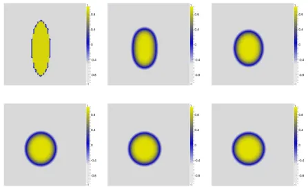
In the first two dimensional example, the piecewise constant initial data on the domain (0,1)2has the shape
of an ellipse. The underlying mesh has 40×40 elements. We useP1 functions, periodic boundary conditions
andγ= 0.001. We observe that the ellipse evolves into a sphere minimizing the length of the transition layer, see Fig. 1.
Figure 1. Evolution of an ellipse at time 0.0,0.05,0.10,0.15,0.20,0.25
6.3.3. Example in 2d with convection
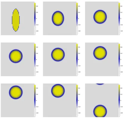
In the second example, we introduce a velocity fieldvto the same initial dataϕ0as in the previous example.
We set v = (0,2x1(x1−1))T. Again the domain is (0,1)2, discretized by a 40×40 mesh, and γ is set to
Figure 2. Evolution of an ellipse at timet= 0.0,0.1, ...,0.7 and end timet= 1.5
6.4.
Summary
The LDG method from [25] combined with an upwind flux for the advection term was shown to be capable of approximating the Cahn–Hilliard equation with additional advection. The code used for the simulations can be run in parallel and can easily be extended with local mesh refinement. However, one has to mention that this approach suffers some drawbacks. We observed a severe time step restriction due to the higher order derivatives. To achieve stability of the computations a time step restriction of the form ∆t≤C∆x4 was required. On the
one hand, this time step restriction is not as bad as it seems, because C ∼γ−1 and in practice one will use
∆x∼γ1/2. On the other hand, for this choice the time step restriction is still ∆t≤C∆x2withC=O(1), which
of the full operator, the overall computational costs in some cases may become similar to those of an explicit scheme with a much smaller time step. To overcome this problem one can implement the actual Jacobi matrix of the discrete operator. This will enable the use of standard preconditioning techniques and in each iteration only one matrix–vector multiplication will be needed in comparison to four grid iterations. The assembling of the Jacobian is not easy because the LDG scheme leads to a large number of matrix entries in the case of 4th order derivatives. Therefore, the so–called CDG method presented in [22], which leads to a simpler and more sparse matrix structure, could be a way to overcome these difficulties.
References
[1] H. Abels. Diffuse interface models for two–phase flows of viscous incompressible fluids, 2007. Lecture Notes, Max Planck Institute for Mathematics in the Sciences, No. 36/2007.
[2] H. Abels, H. Garcke, and G. Gr¨un. Thermodynamically consistent frame indifferent diffuse interface models for incompressible two-phase flows with different densities.Math. Models Methods Appl. Sci., 22:1150013 (40 pages), 2012.
[3] R. Abeyaratne and J. K. Knowles. Kinetic relations and the propagation of phase boundaries in solids.Arch. Rational Mech. Anal., 114(2):119–154, 1991.
[4] G. L. Aki, W. Dreyer, J. Giesselmann, and C. Kraus. An incompressible diffuse model with phase transition. in preparation. [5] H. W. Alt. The entropy principle for interfaces. Fluids and solids.Adv. Math. Sci. Appl., 19(2):585–663, 2009.
[6] D. M. Anderson, G. B. McFadden, and A. A. Wheeler. Diffuse–interface methods in fluid mechanics. InAnnual review of fluid mechanics, Vol. 30, pages 139–165. 1998.
[7] F. Boyer. A theoretical and numerical model for the study of incompressible mixture flows.Computers and Fluids, 31(1):41–68, 2002.
[8] G. Caginalp and P. C. Fife. Dynamics of layered interfaces arising from phase boundaries.SIAM J. Appl. Math., 48(3):506–518, 1988.
[9] J. W. Cahn and J. E. Hilliard. Free Energy of a Nonuniform System. I. Interfacial Free Energy.J. Chem. Phys., 28(2):258–267, 1958.
[10] D. Diehl.Higher order schemes for simulation of compressible liquid–vapor flows with phase change. PhD thesis, Universit¨at Freiburg, 2007. http://www.freidok.uni-freiburg.de/volltexte/3762/.
[11] H. Ding, P.D.M. Spelt, and C. Shu. Diffuse interface model for incompressible two–phase flows with large density ratios.J. Comp. Phys., 226(2):2078–2095, 2007.
[12] W. Dreyer, J. Giesselmann, C. Kraus, and C. Rohde. Asymptotic analysis for Korteweg models. Interfaces Free Bound., 14:105–143, 2012.
[13] W. Dreyer and C. Kraus. On the van der Waals–Cahn–Hilliard phase–field model and its equilibria conditions in the sharp interface limit.Proc. R. Soc. Edinb., Sect. A, Math., 140(6):1161–1186, 2010.
[14] M. E. Gurtin, D. Polignone, and J. Vi˜nals. Two–phase binary fluids and immiscible fluids described by an order parameter.
Math. Models Methods Appl. Sci., 6(6):815–831, 1996.
[15] K. Hermsd¨orfer, C. Kraus, and D. Kr¨oner. Interface conditions for limits of the Navier–Stokes–Korteweg model.Interfaces Free Bound., 13(2):239–254, 2011.
[16] P. C. Hohenberg and B. I. Halperin. Theory of dynamic critical phenomena.Rev. Mod. Phys., 49:435–479, 1977.
[17] T. Y. Hou, J. S. Lowengrub, and M. J. Shelley. The long–time motion of vortex sheets with surface tension.Phys. Fluids, 9(7):1933–1954, 1997.
[18] D. Kr¨oner.Numerical Schemes for Conservation Laws. Wiley & Teubner, 1997.
[19] P. G. LeFloch. Hyperbolic systems of conservation laws. The theory of classical and nonclassical shock waves. Lectures in Mathematics ETH Z¨urich. Birkh¨auser Verlag, Basel, 2002.
[20] J. Lowengrub and L. Truskinovsky. Quasi–incompressible Cahn–Hilliard fluids and topological transitions.R. Soc. Lond. Proc. Ser. A Math. Phys. Eng. Sci., 454(1978):2617–2654, 1998.
[21] N.C. Owen, J. Rubinstein, and P. Sternberg. Minimizers and gradient flows for singularly perturbed bi–stable potentials with a Dirichlet condition.Proc. R. Soc. Lond., Ser. A, 429(1877):505–532, 1990.
[22] J. Peraire and P.-O. Persson. The compact discontinuous Galerkin (CDG) method for elliptic problems.SIAM J. Sci. Comput., 30(4):806–1824, 2008.
[23] P. Sternberg. The effect of a singular perturbation on nonconvex variational problems.Arch. Ration. Mech. Anal., 101(3):209– 260, 1988.
[24] J. D. Van der Waals. Thermodynamische theorie der kapillarit¨at unter voraussetzung stetiger dichte¨anderung.Z. Phys. Chem, 13:657–725, 1894.