A Two-Phase Hybrid Heuristic Method for a Multi-Depot Inventory-Routing Problem

A Two-Phase Hybrid Heuristic Method for a Multi-Depot

Inventory-Routing Problem

Amir-Saeed Nikkhah Qamsari 1_{, Seyyed-Mahdi Hosseini-Motlagh}2_{, Abbas Jokar} 3

Received: 27. 10. 2016 Accepted: 25. 01. 2017

Abstract

In this study, a two phase hybrid heuristic approach was proposed to solve the multi-depot multi-vehicle inventory routing problem (MDMVIRP). Inventory routing problem (IRP) is one of the major issues in the supply chain networks that arise in the context of vendor managed systems (VMI) The MDMVIRP combines inventory management and routing decision. We are given on input a fleet of homogeneous vehicles, in which any of these vehicles have a capacity and a fixed cost. Also, a set of distribution centers with restricted capacities are responsible to serve the customer’s demands, which are known for distributer at beginning of each period. The problem consists of determining the delivery quantity to the customers at each period and the routes to be performed to satisfy the demand of the customers. The objective function of this problem is to minimize sum of the holding cost at distributer centers and the customers, and of the transportation costs associated to the preformed routes. In the proposed hybrid heuristic method, after a Construction phase (first phase) a modified variable neighborhood search algorithm (VNS), with distinct neighborhood structures, is used during the improvement phase (second phase). Moreover, we use simulated annealing (SA) concept to avoid that the solution remains in a local optimum for a given number of iterations. Computational results on benchmark instances that adopt from the literature of IRP indicate that the proposed algorithm is capable to find, within reasonable computing time, several solutions gained by the approaches that applied in the previous published studies.

Keywords: Inventory-routing problem, variable neighborhood search, two-phase heuristic

Corresponding author: [email protected]

1. MSc. Student, School of Industrial Engineering, Iran University of Science and Technology, Tehran, Iran

2. Assistant Professor, School of Industrial Engineering, Iran University of Science and Technology, Tehran, Iran

A Two-Phase Hybrid Heuristic Method for a Multi-Depot Inventory-Routing …

1.

Introduction

Collaboration between all supply chain partners is one of the most important strategies for obtaining competitive advantage. Vendor managed inventory (VMI) system deals with collaboration between a distributer and its customers [Hosseini-Motlagh et al. 2015]. Under VMI policy, the distributer decides on the order quantity and products delivery time to the

customers. Also the vendor takes the

responsibility for determining the inventory level of its customers to prevent any shortage. This approach is often defined as a win-win situation for the supplier and its customers in which suppliers can reduce total cost considerably including distribution and holding costs by integrating transportation decisions between different customers. In addition, retailers do not assign the resources to inventory control.

In the literature, the problem in which transportation and inventory management decisions are integrated simultaneously is called the inventory routing problem (IRP) that is classified in the context of VMI systems. Under this strategy, the vendor is free to decide on how much to deliver to its customers and when to visit each of them. In other words, the vendor guarantees that stock out cannot occur on its customers' side during the time horizon. In the last decade, IRP has received much attention in this research area. There are many applications for IRP in a wide variety of industries such as food distribution, perishable items[Saremi et al. 2015] [Majidi et al. 2015; Hosseini-Motlagh et al. 2017; Majidi et al. 2017], blood[Jokar and Motlagh, 2015; Cheraghi and Hosseini-Motlagh, 2017] and [Jokar and Hosseini Hosseini-Motlagh, 2015], waste organic oil, pharmaceutic Items [Riahi et al., 2013], fuel and automobile components.

One of the first studies on IRP was done by [Bell et al.1998]. Since then, several variants of IRP have been described in the literature, mainly depending on the number of depots (one or multiple), the number of vehicles to visit all

customers (one versus multiple), the nature of the demand function involved (deterministic or stochastic) and the length of the time horizon (finite versus infinite). See for more details [Anderson et al. 2010] and [Coelho et al. 2013].

In the field of exact methods, the first branch and cut algorithm was proposed by [Archetti et al. 2007] for the basic IRP (with a single depot and a single vehicle). Later, it was improved by [Solyalı and Süral, 2011] who used a stronger formulation and a heuristic method to obtain an initial upper bound for the branch and cut algorithm. [Coelho and Laporte, 2013] and [Adulyasak et. al, 2013] introduced an extension of the formulation in [Archetti et al. 2007] for multiple vehicles IRP and solved it by the branch-and-cut algorithm.

Amir-Saeed Nikkhah Qamsari, Seyyed-Mahdi Hosseini-Motlagh, Abbas Jokar

function of the inventory age. [Shabani and Nakhai,2016] introduced an efficient population-based simulated annealing algorithm (PBSA) for Periodic IRP with multiple products. They compared the computational results of the proposed algorithm with simulated annealing (SA) and genetic algorithm (GA).

Our Inventory routing problem literature review researches indicate the leakage of studies in which, the advantage of multiple distribution centers are considered.

[Soysal et al. 2016] proposed the multi-depot IRP for perishable products in the food logistics systems. However, they have only solved the problem with the limited number of customers and depots. In this paper, the IRP model with the advantage of considering multiple distribution centers is enhanced and an effective algorithm for solving the problem at the more reasonable time in the large scales is proposed consequently. Therefore, a multi-depot multi - vehicle IRP problem (MDMVIRP) in which customers' demands are known at the beginning of the time horizon is considered and Moreover, a two-phase heuristic method based on variable neighborhood Search and simulated annealing, which we refer as a two-phase VNS-SA is proposed in this article. Further parts of the paper is organized as

follows. Section two is devoted to the mathematical model. The heuristic algorithm is propsed in section 3 and Comprehensive computational results are presented in Section 4. Finally, conclusions and future research directions are provided in section 5.

2. Problem Description

A mixed-integer linear programming model for the multi-depot, multi-vehicle Inventory Routing problem is addressed in this section. As indicated in (Coelho et al. 2012), it is possible to modify this formulation in order to consider the multi-depot option. This problem is defined on a

graph 𝐺 = (𝑁, 𝐸) , where 𝑁 =

{1, … . |𝑛|, … , |𝑚 + 𝑛|} is composed of the vertex set 𝑁 in which the nodes {1,..,n} represent suppliers (depots) and the remaining nodes denote the retailers and 𝐸{(𝑖, 𝑗): 𝑖, 𝑗 ∈ 𝑁, 𝑖 ≠ 𝑗} is the set of arcs. Meanwhile, in the following we applied abbreviation 𝐸(𝑆) = {(𝑖, 𝑗) ∈ 𝐸: 𝑖 ∈

𝑆, 𝑗 ∈ 𝑆} in which the notation 𝑆 represents arbitrary node set. Moreover {𝑑1𝑑2} are an arbitrary subset of depot set. The storage capacity of all retailers is limited. Furthermore, the demand of all retailers is assumed to be known over all periods.

Sets

Retailers' set

𝑅

Set of depots

𝐷

Set of all points

(𝑅 ∪ 𝐷)

𝑁

Set of time periods

𝑇

Set of vehicles

𝐾

Parameters

Travel cost from retailer/depot

i

to retailer/depot

𝑗

𝑖 ∈ 𝑁, 𝑗 ∈ 𝑁

; satisfying triangular

inequality;

𝑐

+ 𝑐

≥ 𝑐

𝑐

Holding cost in period

𝑡

per unit for

𝑖 ∈ 𝑅

ℎ

Demand of retailer

𝑖

in period

𝑡

for

𝑡 ∈ 𝑇, 𝑖 ∈ 𝑅

𝑟

available product at depot

𝑖 ∈ 𝐷

in period

𝑇

𝑟́

Storage capacity of retailer

𝑖

A Two-Phase Hybrid Heuristic Method for a Multi-Depot Inventory-Routing …

Storage capacity of depot

𝑖

𝑈́

Vehicle capacity

𝑄

𝐼

initial inventory level of customer i

Variables

1 if vehicle

𝑘

along arc

(𝑖, 𝑗)

𝑖 ∈ 𝑁, 𝑗 ∈ 𝑁

and originating from depot

𝑑

and otherwise , 0

𝑦

1, if vehicle k originating from depot d visits point i in period t and otherwise,0

𝑧

Inventory amount of node (supplier or retailer) i in period t

𝐼

The delivered amount to retailer i by vehicle k originating from depot d in period t

𝑞

inventory amount of depot d in period t

𝐼

́

𝑀𝑖𝑛 = ∑

𝐼

́

𝐼

́

́

∑ ∑

∀ 𝑡 ∈ 𝑇, ∀𝑑,

(2)

𝐼𝑖𝑡= 𝐼𝑖,𝑡−1− 𝑟𝑖𝑡+ ∑ ∑ 𝑞𝑖𝑑 𝑘𝑡 𝑑∈𝐷 𝑘∈𝐾

∀ 𝑖 ∈ 𝑅 , 𝑡 ∈ 𝑇,

(3)

𝐼𝑖𝑡≥ 0 ∀ 𝑖 ∈ 𝑁 , 𝑡 ∈ 𝑇 ₍₄₎

∑ 𝑞𝑖𝑑𝑘𝑡≥ 𝑈𝑖∑ 𝑧𝑖𝑡𝑘− 𝐼𝑖,𝑡−1 𝑘∈𝐾

𝑘∈𝐾

∀ 𝑖 ∈ 𝑅 , 𝑡 ∈ 𝑇

(5)

∑ ∑ 𝑞𝑖𝑑𝑘𝑡 𝑑∈𝐷

≤ 𝑈𝑖− 𝐼𝑖,𝑡−1 𝑘∈𝐾

∀ 𝑖 ∈ 𝑅, 𝑡 ∈ 𝑇

(6)

𝑞𝑖𝑑𝑡𝑘≤ 𝑈𝑖𝑧𝑖𝑑𝑡𝑘 ∀ 𝑖 ∈ 𝑅 , 𝑑 ∈ 𝐷, 𝑡 ∈ 𝑇 , 𝑘 ∈ 𝐾 ₍₇₎

∑ ∑ 𝑞𝑖𝑑𝑘𝑡 𝑑∈𝐷

≤ 𝑄𝑘 𝑖∈𝑁́

∀ 𝑡 ∈ 𝑇 , 𝑘 ∈ 𝐾

(8)

∑ ∑ ∑ 𝑦𝑖𝑗𝑑𝑘𝑡 𝑗∈𝑅 𝑑∈𝐷 𝑘∈𝐾

≤ 1 ∀ 𝑖 ∈ 𝑅, 𝑡 ∈ 𝑇

(9)

∑ 𝑦𝑖𝑗𝑑𝑘𝑡 𝑗:(𝑖,𝑗)∈𝐸

= 2𝑧𝑖𝑑𝑡𝑘 ∀ 𝑖 ∈ 𝑁 , 𝑑 ∈ 𝐷, 𝑡 ∈ 𝑇 , 𝑘 ∈ 𝐾

(10)

∑ 𝑦𝑖𝑗𝑘𝑡≤ ∑ 𝑧𝑖𝑑𝑡𝑘 𝑖∈𝑆

−

𝑗:(𝑖,𝑗)∈𝐸(𝑆)

𝑧𝑠𝑑𝑡𝑘 𝑠 ⊆ 𝑁́, 𝑠 ∈ 𝑆, 𝑘 ∈ 𝐾, 𝑡 ∈ 𝑇 ₍₁₁₎

𝑧𝑖𝑑𝑡𝑘∈ {0,1} ∀ 𝑖 ∈ 𝑁 , 𝑡 ∈ 𝑇 , 𝑑 ∈ 𝐷, 𝑘 ∈ 𝐾 ₍₁₂₎

∑ ∑ ∑ 𝑦𝑖𝑗𝑑𝑘𝑡 𝑖∈𝑅 𝑑∈𝐷 𝑘∈𝐾

≤ 1 ∀ 𝑗 ∈ 𝑅, 𝑡 ∈ 𝑇 ₍₁₃₎

𝑦𝑖𝑗𝑑𝑘𝑡 ∈ {0,1} {𝑖, 𝑗} ∈ 𝐸 𝑡 ∈ 𝑇 , 𝑑 ∈ 𝐷, 𝑘 ∈ 𝐾 ₍₁₄₎

𝑦𝑑1𝑗𝑑2𝑘𝑡 = 0 ∀ 𝑑 ∈ 𝐷 , 𝑡 ∈ 𝑇 , 𝑘 ∈ 𝐾 , ∀𝑗 ∈ 𝑁 ₍₁₅₎

𝑦𝑖𝑑1𝑑2𝑘𝑡 = 0 ∀ 𝑑 ∈ 𝐷 , 𝑡 ∈ 𝑇 , 𝑘 ∈ 𝐾 , ∀𝑗 ∈ 𝑁 ₍₁₆₎

Amir-Saeed Nikkhah Qamsari, Seyyed-Mahdi Hosseini-Motlagh, Abbas Jokar

In this model, the aim of the objective function (1) is to minimize the total cost including inventory and transportation costs. The inventory levels for both the suppliers and the retailers at the end of period 𝑡 are defined by constraints (2) and (3). Constraints (4) induce the absence of shortage at the suppliers and the retailers' sides. Constraints (5) and (6) ensure that if customer 𝑖 is visited in period𝑡, the delivered quantity does not exceed the customer's inventory capacity. Constraints (7) limit the available production in each depot. Constraints

(8) ensure that the demand amounts must not exceed the vehicle's capacities. Constraints (9) −

(11) are the routing constraints. Constraints

(12) − (14) define the type of decision variables. Constraints(15) and (16) institute that there is no arc from depots or customers to itself consequently using any type of vehicles. Constraints (17) ensure that at most one vehicle type originating from a given depot can meet customer𝑗.

3. Proposed Method: Two-phase

VNS-SA for the MDMVIRP

The variable neighborhood search (VNS) algorithm, as a meta-heuristic method, was developed by [Mladenović & Hansen, 1997]. The basic idea is to change neighborhood systematically within a local search algorithm. This implies that several neighborhoods are used to search for the solution improvement. In this paper, we propose a two-phase heuristic method based on VNS and SA algorithms to solve MDMVIRP, namely the two-phase VNS-SA method. As it can be seen in Algorithm 1, in the first phase, an initial solution is made through a constructive heuristic method. Then, the initial solution will be improved by modified VNS method. The two phases are described in the following

Algorithm 1. General structure of the proposed method 1 Start

2 Generate Initial solution (first phase) 3 Repeat (second phase)

4 Update 𝑇

5 Loop (VNS structure) 6 Set 𝑘 ← 1;

7 Generate a neighbor solution 𝑥̇ from the kth _{structure of 𝑥}

8 Compute ∆= 𝑓(𝑥́) − 𝑓(𝑥) and generate r (random number between (0,1)) 9 _{If (∆< 0) 𝑜𝑟 (𝑒}−∆⁄𝑇 > 𝑟) then (𝑥 ← 𝑥́), set 𝑘 ← 1; otherwise set 𝑘 ← 𝑘 +1; 10 End loop (until 𝑘 = 𝑘𝑚𝑎𝑥)

11 Loop (Local search structure) 12 Set 𝑙 ← 1;

13 Generate a neighbor solution 𝑥̇ from a random local search of 𝑥

14 Compute ∆= 𝑓(𝑥́) − 𝑓(𝑥) and generate r (random number between (0,1)) 15 _{If (∆< 0) 𝑜𝑟 (𝑒}−∆⁄𝑇_{> 𝑟) then (𝑥 ← 𝑥́)}

16 Set 𝑙 ← 𝑙 +1

17 End loop (until 𝑙 = 𝑙𝑚𝑎𝑥)

A Two-Phase Hybrid Heuristic Method for a Multi-Depot Inventory-Routing …

3.1. Phase 1: Construction of Initial

Solution (IS)

, this phase is divided into two steps, In order

to gain the IS. In the first step, a heuristic

method is performed to solve a capacitated

vehicle routing problem period by period. It

means that, in this step, inventory decisions

will not be taken into consideration. In the

second one, we propose a heuristic procedure

that can be used to improve the IS, which is

generated in the previous step, by considering

the inventory aspect of the problem. In the

heuristic procedure, in a certain period

𝑡

, a

visited retailer will be removed from the

route if it results in reducing the total cost. It

is important to note that the amounts of

quantity of the retailers' demands had to be

satisfied in the previous period. The

procedure is repeated until no more

improvement is possible.

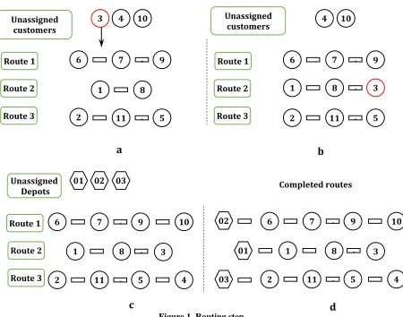
Routing step:

First of all, this step starts by building a

certain number of empty routes based on the

number of the available vehicles. Then,

unassigned customers are selected one by one

(

Fig. 1a

) and inserted into the feasible route

with lower cost (

Fig. 1b

). After that, each

route is assigned to the closest depot with

3 4 10

6 7 ₁ 9

1 8

2 11 ₁ 5

Unassigned customers

Route 1

Route 2

Route 3

4 10

6 7 ₁ 9

2 11 ₁ 5

Unassigned customers

Route 1

Route 2

Route 3

1 8 ₁ 3

a

b

01 02 03

6 7 ₁ 9

2 11 ₁ 5

Unassigned Depots

Route 1

Route 2

Route 3

10

4 3

1 8 ₁ 01

6 7 ₁ 9

2 11 ₁ 5

10

4 3

1 8 ₁

02

03

Completed routes

c

d

Amir-Saeed Nikkhah Qamsari, Seyyed-Mahdi Hosseini-Motlagh, Abbas Jokar

enough residual capacity (

Fig. 1c

and

Fig.

1d

)., the heuristic approach is repeated, For

each period.

3.2. Phase 2: Improvement Phase

The initial solution of the first phase is

improved by the proposed heuristic method.

In the second phase, our proposed scheme is

composed of two parts. At first, a modified

variable neighborhood search algorithm is

used to improve the solution by using a set of

neighborhood structures then, a local search

algorithm is used to escape from the local

optimality. In all over of this phase, the

new

neighborhood

solution

will be accepted after

being compared with the current solution.

This acceptance mechanism is based on the

simulated annealing acceptance criteria

The

heuristic procedure details are described as

follow:

Modified Variable Neighborhood Search

The VNS begins with the initial solution and

tries to iteratively improve the current

solution and reach a better neighboring

solution by using several neighborhood

structures. In our implementation, the

neighborhood is started with a first

improvement strategy and the algorithm will

terminate if no better solution is found. We

use six different neighborhood structures

within the space of the solution. In this

section, we propose a new combination of

using these neighborhood structures in the

context of Inventory routing problem.

Meanwhile, we introduce 2 new structures

(

𝑬

𝑎𝑛𝑑 𝑬

)

which have not already applied

in the literature. Notably, these combinations

have not existed in the literature of inventory

routing problems.

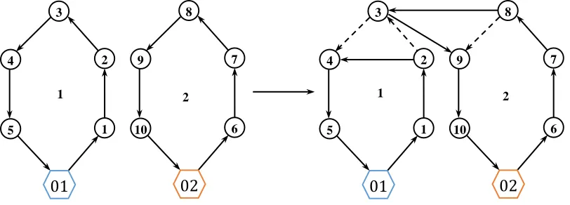
Reposition Neighborhood (E

)

In this structure, to construct a neighbor of

the current solution, a customer is removed

from its route and inserted to a different

position in the same route or another route

planned at the same period. In Figure 2,

customer 3 is moved from the route (1) to

route (2) at the same

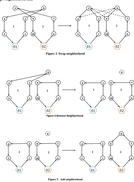
. In this structure,

a neighbor of the current solution is obtained

by swapping a customer of one route by a

customer of another route at the same period.

For example, in Figure 3, customer 8 from the

route (2) is exchanged by customer 3 from the

route (1) at the same period.

A neighbor of the solution is gained by

removing a customer of a route. It means that

the demand of the removed customer is

delivered in the previous periods. Therefore,

the transportation cost will decrease and the

inventory costs will increase. For example, as

it is shown in Figure 4, customer 8 is removed

from the route (1).

1 ₂ 1 ₂

4

3

2

5 1

01

9

8

7

10 6

02

4

3

2

5 1

01

9

8

7

10 6

02

A Two-Phase Hybrid Heuristic Method for a Multi-Depot Inventory-Routing …

Swap Neighborhood (E

)

4

3

2

5 1

01

9

8

7

10 6

02

4

3

2

5 1

01

9

8

7

10 6

02

2 1

2 1

Figure 3. Swap neighborhood

4 2

5 1

01

9

8

7

10 6

02

4 2

5 1

01

9

8

7

10 6

02

2 1

2 1

Figure 4.Remove Neighborhood

4 2

5 1

01

9

8

7

10 6

02

4 2

5 1

01

9

8

7

10 6

02

2 1

2 1

Amir-Saeed Nikkhah Qamsari, Seyyed-Mahdi Hosseini-Motlagh, Abbas Jokar

Remove Neighborhood (E

)

The difference between Drop neighborhood

and Remove neighborhood is that in the

latter, the demand of the customer which is

removed is satisfied in the nearest previous

period visited but in the first, the demand of

the customer which is removed is satisfied

exactly in the previous period.

Swap Periodic Neighborhood (E6)

A neighbor of a solution is obtained by

swapping two customers of two routes in

different periods. For example, in Figure 7,

customer 8 in route (2) and period 3 is

swapped by customer 3 in the route (1) and

period 2.

Local Search Algorithm

Since no further improvement occurs in the

previous section, it might have fallen into the

1 3

5 6

01

9

8

7

10 6

01

1 3

5 6

01

9

8

7

10 6

01

2 1

2 1

T=2 T=3 T=2 T=3

8

Figure 6. Drop neighborhood

3

1 3

5 6

01

9

8

7

10 6

02

1 3

5 6

01

9

3

7

10 6

02

2 1

2 1

T=2 T=3 T=2 T=3

8

A Two-Phase Hybrid Heuristic Method for a Multi-Depot Inventory-Routing …

local optimality. , some heuristic local search

methods are used for escaping this trap. Arc

exchange, Depot Exchange, and Partial

Route Drop are three heuristic method which

are used in this section. More details are

described as follows:

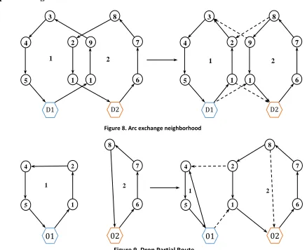
Arc Exchange

In this procedure, a neighbor of the current solution is obtained by exchanging an arc of one route by an arc of another route at the same period. For example, in Figure 8, the arc between customer 9 and customer 10 from the route (1) is exchanged by the arc between customer 1 and customer 2 from the route (2) at the same period

.

Depot Exchange

In this procedure, a neighbor of the current

solution is achieved by swapping the depot of

one route by the depot of another route at the

same period. Similarly, all possible exchange

modes are checked.

Drop Partial Route

In this heuristic procedure, a neighbor of the

solution is defined by removing partial

customers of a route and adding them to a

new position in another route at the same

period. For example, in Figure 9, customers 1

and 2 are removed from the route (1) and are

inserted into the route (2).

2 1

4 2

5 1

01

8

7

6

02

2 1

4 2

5 1

01

8

7

6

02

Figure 9. Drop Partial Route 4

3

2

5 1

D1

9

8

7

1 6

D2

4

3

2

5 1

D1

9

8

7

1 6

D2

Figure 8. Arc exchange neighborhood

2 1

Amir-Saeed Nikkhah Qamsari, Seyyed-Mahdi Hosseini-Motlagh, Abbas Jokar

4. Computational results

Our proposed algorithm was coded in

MATLAB

2014.b

and

computational

experiments were conducted on a platform

Intel Core i5 with 4 GB RAM and 3.4 GHz

processor. Detailed experimental tests were

presented for the introduced algorithm. Due

to randomness nature of our proposed

method, five independent replications were

run on each instance and the minimum

objective value among the five runs is

reported.

To evaluate the quality of our proposed

heuristic method, two benchmark datasets are

employed for the single-depot and

multi-vehicle case generated by Archetti et al.

[Archetti et al, 2007]and the obtained results

are compared with some available results in

the literature including Coelho & Laporte

[Coelho & Laporte, 2013] and Adulyasak et

al. [Adulyasak et al. 2014]. These data sets are

classified by the number of customers and the

planning horizon. In addition, they are divided

into two sets with respect to two levels of

inventory holding costs. It is included six time

periods with 30 customers, and three time

periods with 50 customers. These are

characterized small-n-p-low or small-n-p-high

in which n represent the number of customers,

p represents the number of periods and symbol

low/high is about two levels of inventory

holding costs. The solution results are reported

in Table 1 and Table 2. The first column

demonstrates the instance names. Then, , the

tables provide a gap of the best cost obtained

in five runs of each algorithm in comparison

with the best lower bound (LB) obtained by

Coelho et.al [Coelho et. al., 2012] and the

duration of the best run in seconds. For

example, the deviation of a method A to the

LB is computed as:

𝐺𝑎𝑝(%) = (𝐶𝑜𝑠𝑡(𝐴) − 𝐿𝐵 𝐿𝐵

⁄

) ∗ 100

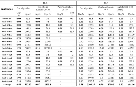
Table 1. Computational results on the (Coelho & Laporte 2013)small instances set, p=3.

instances

K=2 K=3

Our algorithm _{Laporte 2013)} (Coelho & (Adulyasak et al. ₂₀₁₄₎ Our algorithm (Coelho & Laporte ₂₀₁₃₎ (Adulyasak et al. ₂₀₁₄₎

Gap

% Cpu(s) Gap% Cpu (s) Gap%

Cpu

(s) Gap% Cpu(s) Gap % Cpu(s) Gap% Cpu(s)

Small-5-low 0.00 45.6 0.00 3.8 0.00 0.1 0.00 56.8 0.00 4.6 0.00 0.3

Small-10-low 0.00 83.5 0.00 7.6 0.00 1.2 0.00 89.8 0.00 17.4 0.00 6.7

Small-15-low 0.00 123.8 0.00 11.8 0.00 3.3 0.00 127.5 0.00 31.4 0.00 29.2

Small-20-low 0.00 166.3 0.00 24.4 0.00 21.1 0.00 179.9 0.00 220.8 0.00 237.7 Small-25-low 0.00 207.2 0.00 31.6 0.00 55.7 0.00 229.6 0.00 574.2 0.00 639.9

Small-30-low 0.00 244.3 0.00 61.8 - - 0.00 281.6 0.00 1285.8 0.00 1746.9

Small-35-low 0.70 282.8 0.00 56.0 - - 0.00 333.1 0.00 1935.8 0.00 2224.3

Small-40-low 1.10 391.4 0.00 525.0 - - 0.90 447.3 0.00 9092.0 0.00 5569.1

Small-45-low 0.90 513.4 0.00 3867.8 - - 1.90 588.0 0.86 31805 0.00 18549

Small-50-low 1.70 900.2 0.15 10796.3 - - 4.90 1002.7 12.40 42930 4.9 43200

Small-5-high 0.00 43.8 0.00 2.8 0.15 0.2 0.00 40.1 0.00 2.3 0.00 0.3

Small-10-high 0.00 89.5 0.00 5.8 0.00 1.2 0.00 79.7 0.00 12.6 0.00 7.6

Small-15-high 0.00 135.1 0.00 11.6 0.00 3.3 0.00 123.9 0.00 26.0 0.00 24.7

Small-20-high 0.00 172.6 0.00 23.8 0.00 17.3 0.00 171.4 0.00 217.4 0.00 227.6 Small-25-high 0.90 209.3 0.00 30.8 0.00 31.1 0.00 215.1 0.00 1013.6 0.00 646.1

Small-30-high 1.00 248.5 0.00 70.4 - - 0.00 268.8 0.00 1623.4 0.00 966.9

Small-35-high 0.80 285.6 0.00 65.6 - - 0.00 332.2 0.00 2696.0 0.00 1624

Small-40-high 0.20 424.5 0.00 478.5 - - 0.81 451.3 0.00 6312.4 0.00 5638

Small-45-high 1.90 542.2 0.00 1595.0 - - 1.20 597.0 0.4 32820 0.00 13913

Small-50-high 2.10 933.8 0.00 4431.6 - - 1.90 1017.7 4.39 42990 1.5 43200

A Two-Phase Hybrid Heuristic Method for a Multi-Depot Inventory-Routing …

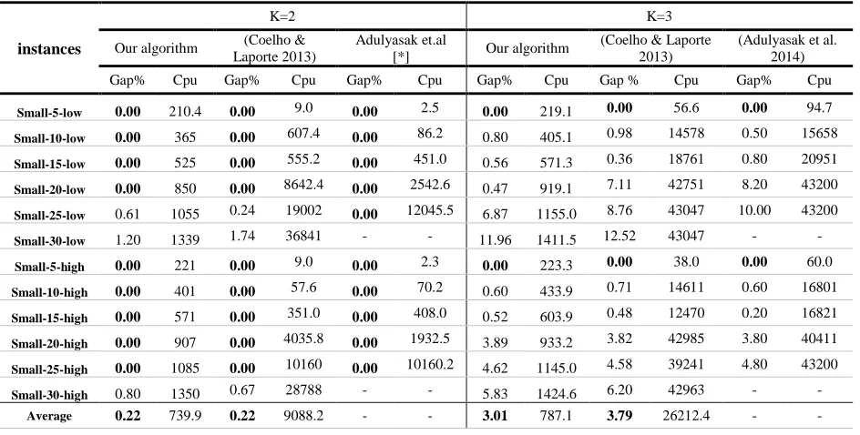
Table 2. Computational results on the (Coelho & Laporte 2013)small instances set, p=6.

instances

K=2 K=3

Our algorithm (Coelho & Laporte 2013)

Adulyasak et.al

[*] Our algorithm

(Coelho & Laporte 2013)

(Adulyasak et al. 2014)

Gap% Cpu Gap% Cpu Gap% Cpu Gap% Cpu Gap % Cpu Gap% Cpu

Small-5-low 0.00 210.4 0.00 9.0 0.00 2.5 0.00 219.1 0.00 56.6 0.00 94.7 Small-10-low 0.00 365 0.00 607.4 0.00 86.2 0.80 405.1 0.98 14578 0.50 15658 Small-15-low 0.00 525 0.00 555.2 0.00 451.0 0.56 571.3 0.36 18761 0.80 20951 Small-20-low 0.00 850 0.00 8642.4 0.00 2542.6 0.47 919.1 7.11 42751 8.20 43200 Small-25-low 0.61 1055 0.24 19002 0.00 12045.5 6.87 1155.0 8.76 43047 10.00 43200 Small-30-low 1.20 1339 1.74 36841 - - 11.96 1411.5 12.52 43047 - - Small-5-high 0.00 221 0.00 9.0 0.00 2.3 0.00 223.3 0.00 38.0 0.00 60.0 Small-10-high 0.00 401 0.00 57.6 0.00 70.2 0.60 433.9 0.71 14611 0.60 16801 Small-15-high 0.00 571 0.00 351.0 0.00 408.0 0.52 603.9 0.48 12470 0.20 16821 Small-20-high 0.00 907 0.00 4035.8 0.00 1932.5 3.89 933.2 3.82 42985 3.80 40411 Small-25-high 0.00 1085 0.00 10160 0.00 10160.2 4.62 1145.0 4.58 39241 4.80 43200 Small-30-high 0.80 1350 0.67 28788 - - 5.83 1424.6 6.20 42963 - -

Average 0.22 739.9 0.22 9088.2 - - 3.01 787.1 3.79 26212.4 - -

The first row shows the number of vehicles

for each instance. The last row displays the

average gap and the mean CPU time for each

algorithm. Numbers in boldface indicate

which methods give the same LB.

As it can be seen in Table 1, for k=2, the

average of gaps obtained by Coelho &

Laporte [Coelho & Laporte, 2013] is lower

than what is obtained in this study. But their

solution time's average is much more than the

proposed method. For k=3, the average of

gaps of the proposed method is lower than the

one obtained by Coelho et.al [Coelho et al.

2013] but is more than the average obtained

by Adulyasak et al.[ Adulyasak et al. 2014].

In Table 2, for k=2, the average of gaps

obtained by Coelho and Laporte [Coelho and

Laporte, 2013] appear to be the same as the

proposed method. However, solution time's

average obtained by these authors is much

more than the proposed method. For k=3, the

average of gaps of the proposed method is the

same as the one obtained by Coelho and

Laporte [Coelho and Laporte, 2013].

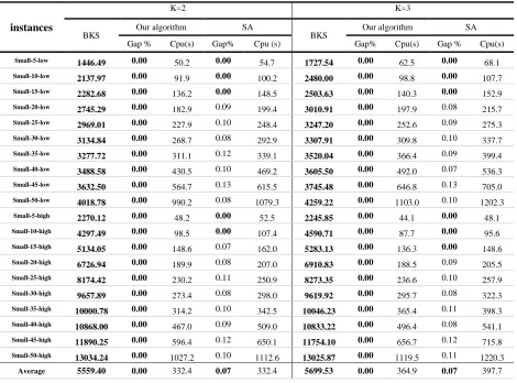
In the second set of the experiments, new

instances for the case with multiple depots

have been generated. In these sets of

instances, modifying the instances proposed

by Coelho et al.[Coelho et al, 2012] were

obligated. In order to solve the multiple

depots IRP, the same algorithm used in the

previous section was applied. Also a

simulated annealing algorithm was applied to

solve the multi-depot IRP. In Tables 3-4 the

comparison between our two-phase VNS-SA

algorithms with the proposed SA method is

provided. Note that "BKS" in the presented

tables represent the best-known solution

which has been founded in the current level

of problem.

Amir-Saeed Nikkhah Qamsari, Seyyed-Mahdi Hosseini-Motlagh, Abbas Jokar

planning horizons T=3 and 6 and the number

of vehicles K=2 and 3 are presented. In each

table, the average percentage gap is

demonstrated.

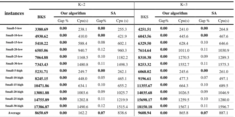
Comparing

the

results

obtained by the proposed method with SA

algorithm has quite interesting results.

Two-phase VNS-SA finds a better solution than

SA and the average gap for the two-phase

VNS-SA is obviously lower.

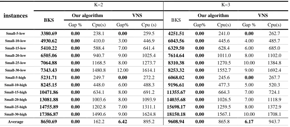
In Tables 5-6, it has been tried to reflect the

effect of a set of local searches used in the

proposed algorithm. For this purpose, a

comparison between solutions under the local

searches and without them for the

multi-depot IRP is provided. The average gap

between the two mentioned strategies in the

same tables is reported to One considerable

point is that the algorithm stops when the

solutions will not be improved by local

searches either. Therefore, the reported gap

describes

the

solution

improvement

percentage via local searches.

Table 3. Computational results on the small instances set for MDMVIRP, p=3.

instances

K=2 K=3

BKS Our algorithm SA BKS Our algorithm SA

Gap % Cpu(s) Gap% Cpu (s) Gap% Cpu(s) Gap % Cpu(s)

Small-5-low _1446.49 0.00 _50.2 0.00 _{54.7 1727.54} 0.00 _62.5 0.00 _68.1

Small-10-low _2137.97 0.00 _91.9 0.00 _{100.2 2480.00} 0.00 _98.8 0.00 _107.7

Small-15-low _2282.68 0.00 _136.2 0.00 _{148.5 2503.63} 0.00 _140.3 0.00 _152.9

Small-20-low _2745.29 0.00 _182.9 0.09 _{199.4 3010.91} 0.00 _197.9 0.08 _215.7

Small-25-low _2969.01 0.00 _227.9 0.10 _{248.4 3247.20} 0.00 _252.6 0.09 _275.3

Small-30-low _3134.84 0.00 _268.7 0.08 _{292.9 3307.91} 0.00 _309.8 0.10 _337.7

Small-35-low _3277.72 0.00 _311.1 0.12 _{339.1 3520.04} 0.00 _366.4 0.09 _399.4

Small-40-low _3488.58 0.00 _430.5 0.10 _{469.2 3605.50} 0.00 _492.0 0.07 _536.3

Small-45-low _3632.50 0.00 _564.7 0.13 _{615.5 3745.48} 0.00 _646.8 0.13 _705.0

Small-50-low _4018.78 0.00 _990.2 0.08 _{1079.3 4259.22} 0.00 _1103.0 0.10 _1202.3

Small-5-high _2270.12 0.00 _48.2 0.00 _{52.5 2245.85} 0.00 _44.1 0.00 _48.1

Small-10-high _4297.49 0.00 _98.5 0.00 _{107.4 4590.71} 0.00 _87.7 0.00 _95.6

Small-15-high _5134.05 0.00 _148.6 0.07 _{162.0 5283.13} 0.00 _136.3 0.00 _148.6

Small-20-high _6726.94 0.00 _189.9 0.08 _{207.0 6910.83} 0.00 _188.5 0.09 _205.5

Small-25-high _8174.42 0.00 _230.2 0.11 _{250.9 8273.35} 0.00 _236.6 0.10 _257.9

Small-30-high _9657.89 0.00 _273.4 0.08 _{298.0 9619.92} 0.00 _295.7 0.08 _322.3

Small-35-high _10000.78 0.00 _314.2 0.10 _{342.5 10046.23} 0.00 _365.4 0.11 _398.3

Small-40-high _10868.00 0.00 _467.0 0.09 _{509.0 10833.22} 0.00 _496.4 0.08 _541.1

Small-45-high _11890.25 0.00 _596.4 0.12 _{650.1 11754.10} 0.00 _656.7 0.12 _715.8

A Two-Phase Hybrid Heuristic Method for a Multi-Depot Inventory-Routing …

Table 4. Computational results on the small instances set for MDMVIRP, p=6.

instances

K=2 K=3

BKS Our algorithm SA BKS Our algorithm SA

Gap % Cpu(s) Gap% Cpu (s) Gap% Cpu(s) Gap % Cpu(s)

Small-5-low _3380.69 0.00 _238.1 0.00 _{255.3 4251.51} 0.00 _241.0 0.00 _264.8

Small-10-low _4930.62 0.00 _410.0 0.00 _{421.9 6043.56} 0.00 _445.6 0.00 _467.6

Small-15-low _5410.22 0.00 _588.4 0.08 _{602.1 6329.50} 0.00 _628.4 0.10 _646.6

Small-20-low _6505.06 0.00 _940.7 0.12 _{960.3 7614.64} 0.00 _1011.0 0.11 _1030.9

Small-25-low _7064.88 0.00 _1168.5 0.10 _{1182.2 8310.38} 0.00 _1270.5 0.09 _1289.3

Small-30-low _7343.43 0.00 _1480.8 0.11 _{1498.3 8253.32} 0.00 _1552.7 0.11 _1575.3

Small-5-high _5231.71 0.00 _249.7 0.00 _{262.1 6068.02} 0.00 _245.6 0.00 _261.0

Small-10-high _8245.15 0.00 _448.0 0.05 _{465.1 9196.61} 0.00 _477.3 0.07 _497.1

Small-15-high _10471.86 0.00 _634.1 0.10 _{655.2 11355.67} 0.00 _664.3 0.10 _689.5

Small-20-high _13081.88 0.00 _1003.6 0.09 _{1025.7 14035.68} 0.00 _1026.5 0.09 _1046.9 Small-25-high _14755.89 0.00 _1202.8 0.11 _{1219.9 15698.17} 0.00 _1259.5 0.10 _1280.0 Small-30-high _17386.87 0.00 _1490.6 0.12 _{1515.4 18150.18} 0.00 _1567.1 0.11 _1596.7 Average 8650.69 0.00 162.2 0.07 838.6 9608.94 0.00 865.8 0.07 887.1

5. Conclusions

A hybrid heuristic algorithm based on the

variable neighborhood search and the

simulated annealing algorithm is introduced

in this study. The proposed algorithm is

comprised of two phases. The first phase

generates an initial solution in which

inventory costs are ignored in step 1. In the

second phase the solution, which is initially

constructed in phase 1, is improved by

applying both a variable neighborhood search

and

a

local

search.

Six

different

neighborhood structures and 3 different local

searches for the proposed algorithm has been

used in this study. The computational tests

showed that this algorithm provides near

optimal solution in the more reasonable time

than the ones obtained by the existing

method. The applications of such proposed

model arise in a wide variety of industries

such as the distribution of blood products,

food distribution to supermarket chains,

delivery of waste organic oil and etc. there

are many issues which can enhance the

models usage in these research area,. Some of

the most significant issues are addressed as

follows:



Considering limited shelf life of

products in the model (perishability)



Transshipment between distribution

centers and customers



Developing the model by adding

pickup and delivery constraints which

leads to more realistic results.

Amir-Saeed Nikkhah Qamsari, Seyyed-Mahdi Hosseini-Motlagh, Abbas Jokar

Table 5. Computational results of the effect of local search on the results, p=3.

Table 6. Computational results of the effect of local search on the results, p=6.

instances

K=2 K=3

BKS Our algorithm VNS BKS Our algorithm VNS

Gap % Cpu(s) Gap% Cpu (s) Gap% Cpu(s) Gap % Cpu(s)

Small-5-low 3380.69 0.00 238.1 0.00 259.5 4251.51 0.00 241.0 0.00 262.7

Small-10-low 4930.62 0.00 410.0 3.00 446.9 6043.56 0.00 445.6 4.00 485.7

Small-15-low 5410.22 0.00 588.4 7.00 641.4 6329.50 0.00 628.4 6.00 685.0

Small-20-low 6505.06 0.00 940.7 9.00 1025.4 7614.64 0.00 1011.0 8.00 1102.0

Small-25-low 7064.88 0.00 1168.5 8.00 1273.7 8310.38 0.00 1270.5 10.00 1384.8

Small-30-low 7343.43 0.00 1480.8 12.00 1614.1 8253.32 0.00 1552.7 9.00 1692.4

Small-5-high 5231.71 0.00 249.7 0.00 272.2 6068.02 0.00 245.6 0.00 267.7

Small-10-high 8245.15 0.00 448.0 6.00 488.3 9196.61 0.00 477.3 5.00 520.3

Small-15-high 10471.86 0.00 634.1 8.00 691.2 11355.67 0.00 664.3 7.00 724.1

Small-20-high 13081.88 0.00 1003.6 8.00 1093.9 14035.68 0.00 1026.5 7.00 1118.9 Small-25-high 14755.89 0.00 1202.8 7.00 1311.1 15698.17 0.00 1259.5 8.00 1372.9 Small-30-high 17386.87 0.00 1490.6 9.00 1624.8 18150.18 0.00 1567.1 10.00 1708.1 Average 8650.69 0.00 162.2 6.42 895.2 9608.94 0.00 865.8 6.17 943.7 instances

K=2 K=3

BKS Our algorithm VNS BKS Our algorithm VNS

Gap % Cpu(s) Gap% Cpu (s) Gap% Cpu(s) Gap % Cpu(s)

Small-5-low 1446.49 0.00 50.2 0.00 57.7 1727.54 0.00 62.5 0.00 73.1

Small-10-low 2137.97 0.00 91.9 0.00 105.7 2480.00 0.00 98.8 0.00 115.6

Small-15-low 2282.68 0.00 136.2 4.00 156.6 2503.63 0.00 140.3 3.00 164.2

Small-20-low 2745.29 0.00 182.9 3.00 210.3 3010.91 0.00 197.9 4.00 231.5

Small-25-low 2969.01 0.00 227.9 8.00 262.1 3247.20 0.00 252.6 6.00 295.5

Small-30-low 3134.84 0.00 268.7 6.00 309.0 3307.91 0.00 309.8 6.00 362.5

Small-35-low 3277.72 0.00 311.1 9.00 357.8 3520.04 0.00 366.4 9.00 428.7

Small-40-low 3488.58 0.00 430.5 8.00 495.1 3605.50 0.00 492.0 6.00 575.6

Small-45-low 3632.50 0.00 564.7 9.00 649.4 3745.48 0.00 646.8 7.00 756.8

Small-50-low 4018.78 0.00 990.2 6.00 1138.7 4259.22 0.00 1103.0 8.00 1290.5

Small-5-high 2270.12 0.00 48.2 0.00 55.4 2245.85 0.00 44.1 0.00 51.6

Small-10-high 4297.49 0.00 98.5 3.00 113.3 4590.71 0.00 87.7 0.00 102.6

Small-15-high 5134.05 0.00 148.6 4.00 170.9 5283.13 0.00 136.3 4.00 159.5

Small-20-high 6726.94 0.00 189.9 6.00 218.4 6910.83 0.00 188.5 3.00 220.5

Small-25-high 8174.42 0.00 230.2 7.00 264.7 8273.35 0.00 236.6 8.00 276.8

Small-30-high 9657.89 0.00 273.4 8.00 314.4 9619.92 0.00 295.7 8.00 346.0

Small-35-high 10000.78 0.00 314.2 6.00 361.3 10046.23 0.00 365.4 9.00 427.5

Small-40-high 10868.00 0.00 467.0 7.00 537.1 10833.22 0.00 496.4 8.00 580.8

Small-45-high 11890.25 0.00 596.4 8.00 685.9 11754.10 0.00 656.7 9.00 768.3

A Two-Phase Hybrid Heuristic Method for a Multi-Depot Inventory-Routing …

6

.

References

-Adulyasak, Y., Cordeau, J. F. and Jans, R.

(2013) "Formulations and branch-and-cut algorithms for multivehicle production and inventory routing problems", INFORMS Journal on Computing, Vol.26, No.1, pp.103-120.

-Andersson, H., Hoff, A., Christiansen, M., Hasle, G. and Løkketangen, A. (2010) "Industrial aspects and literature survey:

Combined inventory management and

routing", Computers and Operations Research, Vol.37, No.9, pp.1515–1536. Available at: http://dx.doi.org/10.1016/j.

-Archetti, C., Bertazzi, L., Laporte, G. and Speranza, M. G. (2007) "A branch-and-cut algorithm for a vendor-managed inventory-routing problem", Transportation Science, Vol.41, No.3, pp.382–391. Available at: http://pubsonline.informs.org/doi/abs/10.128 7/trsc.1060.0188.

-Archetti, C., Bertazzi, L. and Speranza, M. G. (2012) "A hybrid heuristic for an inventory routing problem". , INFORMS Journal on

Computing, Vol.24, No.1, pp.101–116.

-Bell, W.J., Dalberto, L. M., Fisher, M.L., Greenfield, A.J., Jaikumar, R., Kedia, P., Mack, R.G. and Prutzman, P.J. (1983). "Improving the distribution of industrial gases with an on-line computerized routing and scheduling optimizer", Interfaces, Vol.13, No.6, pp.4–23.

-Cheraghi, S. and Hosseini-Motlagh, S.-M. (2017) " Optimal Blood Transportation in Disaster Relief Considering Facility Disruption and Route Reliability under Uncertainty", International Journal of Transportation Engineering, Vol. 4, No. 3, pp.225-254.

-Coelho, L.C., Cordeau, J.F. and Laporte, G. (2012) "Consistency in multi-vehicle inventory-routing", Transportation Research Part C: Emerging Technologies, Vol.24,

pp.270–287. Available at:

http://dx.doi.org/10.1016/j.trc.2012.03.007.

-Coelho, L.C. and Laporte, G. (2013) "The exact solution of several classes of inventory-routing problems", Computers and Operations Research, Vol.40,No.2, pp.558–

565. Available at:

http://dx.doi.org/10.1016/j.cor.2012.08.012.

-Cordeau, J. F., Laganà, D., Musmanno, R., and Vocaturo, F. (2014) " A decomposition-based heuristic for the multiple-product inventory-routing problem", Computers and Operations Research, Vol.55, pp.153–166.

Available at: htt

p://dx.doi.org/10.1016/j.cor.2014.06.007.

-Hosseini-Motlagh, S.-M., Ahadpour, P. and Haeri, A. (2015) "Proposing an approach to calculate headway intervals to improve bus fleet scheduling using a data mining algorithm", Journal of Industrial and Systems Engineering, Vol.8, No.4, pp.72–86.

Hosseini-Motlagh, S. M., Majidi, S., Yaghoubi, S., & Jokar, A. (2017) "Fuzzy green vehicle routing problem with simultaneous pickup-delivery and time windows". RAIRO-Operations Research.

Available at:

https://doi.org/10.1051/ro/2017007

-Huang, S.-H. and Lin, P.-C. (2010) "A modified ant colony optimization algorithm for multi-item inventory routing problems with demand uncertainty", Transportation

Research Part E: Logistics and

Transportation Review, Vol.46, No.5,

pp.598–611. Available at:

http://dx.doi.org/10.1016/j.tre.2010.01.006.

-Jokar, A. and Hosseini-Motlagh, S.-M. (2015) "Impact of capacity of mobile units on blood supply chain performance: Results from a robust analysis", International Journal of Hospital Research, Vol.4, No.3, pp.101– 105.

Amir-Saeed Nikkhah Qamsari, Seyyed-Mahdi Hosseini-Motlagh, Abbas Jokar

Journal of Management and Sustainability, Vol.2, No.2, pp.219.

-Liu, S. C. and Lee, S. B. (2003) "A two-phase heuristic method for the multi-depot location routing problem taking inventory control decisions into consideration",

International Journal of Advanced

Manufacturing Technology, Vol.22, No.(11– 12), pp. 941–950.

-Majidi, S., Hosseini-Motlagh, S.-M., Yaghubi,S., Jokar, A. (2015). "An adaptive large neighborhood search heuristic for the green vehicle routing problem with simultaneously pickup and delivery and hard time windows", Journal Of Industrial Engeeniring Research in Production Systems, Vol.3, No.6, pp.149–165.

-Majidi, S., Hosseini-Motlagh, S.-M., Ignatius, J. (2017). "Adaptive Large Neighborhood Search heuristic for Pollution Routing Problem with simultaneous pickup and delivery", Soft Computing, Available at: 10.1007/s00500-017-2535-5

-Mirzaei, S. and Seifi, A. (2015). "Considering lost sale in inventory routing problems for perishable goods", Computers and Industrial Engineering, Vol.87 (May),

pp.213–227. Available at:

http://dx.doi.org/10.1016/j.cie.2015.05.010.

-Mirzapour Al-e-hashem, S.M.J. and Rekik, Y. (2014) "Multi-product multi-period

inventory routing problem with a

transshipment option: a green approach", International Journal of Production Economics, Vol.157, pp.80–88.

-Mladenović, N. and Hansen, P. (1997) "Variable neighborhood search", Computers & Operations Research, Vol.24, No.11, pp.1097–1100.

-Park, Y.-B., Yoo, J.-S. and Park, H.-S. (2016) "A genetic algorithm for the vendor-managed inventory routing problem with lost sales", Expert Systems with Applications, Vol.53, pp.149–159.

-Poorjafari, V., Long Yue, W., and Holyoak, N. (2016) "A novel method for measuring the quality of temporal integration in public transport systems", International Journal of Transportation Engineereing , Vol.4, No.1, pp.53-59.

-Riahi N., Hosseini-Motlagh, S.-M., Teimourpour, B., (2013) " Three-phase Hybrid Times Series Modeling Framework for Improved Hospital Inventory Demand Forecast", International Journal of Hospital Research Vol. 2, No. 3, pp.130-138

-Saremi, S., Hosseini-Motlagh, S.-M.,S. and Sadjadi, S.J. (2016) "A reschedule design for disrupted liner ships considering ports demand and CO2 emissions : the case study of islamic republic of Iran shipping lines (IRISL)", Journal of Industrial and Systems Engineering, Vol.9, No.1, pp.126–148.

-Shaabani, H. and Kamalabadi, I. N. (2016) "An efficient population-based simulated annealing algorithm for the multi-product multi-retailer perishable inventory routing problem", Computers and Industrial Engineering, Vol.99, pp.189–201. Available at:

http://dx.doi.org/10.1016/j.cie.2016.07.022.

-Solyali, Ǒguz and Süral, H. (2011) "A branch-and-cut algorithm using a strong formulation and an a priori tour-based heuristic for an inventory-routing problem", Transportation Science,Vol.45, No.3, pp.335–345.