Anisotropic Diffusion in Toroidal geometries*

M. Campos Pinto and F. Charles, Editors

ANISOTROPIC DIFFUSION IN TOROIDAL GEOMETRIES

Ahmed Ratnani

, Emmanuel Franck

, Boniface Nkonga

, Alina Eksaeva

and

Maria Kazakova

Abstract. In this work, we present a new finite element framework for toroidal geometries based on a tensor product description of the 3D basis functions. In the poloidal plan, different discretizations, including B-splines and cubic Hermite-B´ezier surfaces are defined, while for the toroidal direction both Fourier discretization and cubic Hermite-B´ezier elements can be used. In this work, we study the MHD equilibrium by solving the Grad-Shafranov equation, which is the basis and the starting point of any MHD simulation. Then we study the anisotropic diffusion problem in both steady and unsteady states.

1.

Introduction

The context of this work is the simulation and the modeling of nuclear fusion reaction as power source. The aim of magnetic confinement fusion is to develop a power plant that gains energy from the fusion of deuterium and tritium in a magnetically confined plasma. ITER, a tokamak type fusion experiment currently being built in the South of France, is the next step towards this goal. One of the many challenges for the numerical simulation in a tokamak is the modeling and the simulation of magneto-hydrodynamics (MHD) instabilities as disruptions or ELMs [11] [1]. These instabilities which occur at the boundary of the plasma generate a loss of energy and can damage the wall of the tokamak. For this reason it is necessary to understand the behavior of these instabilities and find a way to control them using experiment and simulation. A physical model well suited to describe those large scale instabilities is the set of magneto-hydrodynamic equations (MHD) with resistivity and bi-fluid effects. In the world some codes have been developed to simulate this problem and solve the MHD equations. One of those codes is the JOREK code which implements and solves both some reduced and full MHD models [10] based on assumptions on the velocity and magnetic fields in a toroidal geometry. The equations in the poloidal plane (circular, d-shape or x-point meshes) [6] [5] [7] are discretized using cubic bezier splines and the toroidal discretization use Fourier expansion. In this work, we are interested in the study a small part of the equations used in JOREK which can generate numerical difficulties: the elliptic and parabolic operators, especially the anisotropic diffusion.

In a tokamak, the heat diffusion is mostly in the direction of the magnetic field described by a large toroidal part and a poloidal perturbation (in the JOREK code the toroidal part of magnetic field is assumed constant in time). At the limit (where the ratio between the diffusion in the magnetic field direction and the isotropic diffusion tend to the infinity) the problem is singular [9]. This singularity at the limit generates ill-conditioning, large error in the perpendicular direction and other numerical problems. At the end, we

∗ _{This work has been carried out within the framework of the EUROfusion Consortium and has received funding from the}

Euratom research and training programme 2014-2018 under grant agreement No 633053. The views and opinions expressed herein do not necessarily reflect those of the European Commission.

∗∗_{Corresponding author: ahmed.ratnani@ipp.mpg.de}

1_{Max-Planck Institute f¨ur PlasmaPhysik, Garching, Munich} 2_{Inria Nancy Grand-Est & IRMA, Strasbourg, France}

3_{Laboratoire Jean Dieudonn´e, Universit´e Nice Sophia-Antipolis, Nice, France} 4_{Moscow Engineering & Physics Institute MEPHI, Russia}

5_{Lavrentyev Institute of Hydrodynamics of SB RAS, Russia}

©EDP Sciences, SMAI 2016

want study the discretization of elliptic operators especially the anisotropic diffusion operators with splines on toroidal geometry to understand and identify the main numerical problems linked to these operators and in the future propose numerical solutions for the JOREK code.

In the first part of this paper we will detail the construction of the 3D finite elements (obtained by tensor product 2D ×1D) using a 2D Hermite-B´ezier discretization. The second part is on the discretization of the elliptic Grad-Safranov operator. This operator is important in the JOREK code to obtain the magnetic equilibrium and the toroidal current in the MHD. This operator is also a simplified 2D operator in the cylindrical geometry comparing to the anisotropic diffusion and a first step to study finit element method in the cylindrical coordinates. After the Grad - Shafranov equation we will study the discretization of the anisotropic diffusion equation. These problems are studied on some classical geometries in the tokamak contexts: circular or d-shape poloidal section.

2.

B´

ezier Finite Elements Method

In this section, we present a cubic Hermite-B´ezier finite elements method. We consider the isoparametric setting, where both the geometry and the discrete space are described by the same basis functions, which are cubic Hermite-B´ezier elements. First, we start by recalling B´ezier curves and surfaces. Then we introduce a flexible way to create and manipulate the geometry, thanks to B-splines curves and surfaces. We then explain how to convert a B-spline surface into B´ezier surfaces and finally to the cubic Hermite-B´ezier description. It is very important to keep in mind that the B´ezier surfaces are considered as elements, while the B-spline surface/patch can be decomposed into a structured grid where each element is a B´ezier surface. Hence, a B-spline surface can be viewed as amacro-element.

2.1.

Bezier curves and surfaces

B´ezier curves/surfaces are polynomial parametric curves/surfaces. Since their introduction by B´ezier in 1962, they became very popular in the Computer Aided Design (CAD) community.

A B´ezier curve (also called arc) of degreepis defined as

C(u) =

p

X

i=0

ciBip(u), (2.1)

where (B_ip)_0≤i≤p denote Bernstein polynomials : B_ip(t) =

p i

ti_(1−t)p−i₌ p! i!(p−i)!t

i_(1−t)p−i_{, 0≤t≤1.}

The coefficients (ci)_0≤i≤p are called control points. Among the interesting properties of B´ezier curves, we recall

the affine invariance one: any affine transformation, including translations, rotations and scaling, is applied to the curve by applying it to the control points.

A B´ezier surface of degrees (p, q) is defined as

S(u, v) =

p

X

i=0 q

X

j=0

sijBip(u)B q

j(v), (2.2)

where (Bi)0≤i≤p and (Bj)_0≤j≤q are the Bernstein polynomials of degreespandq, respectively. (sij)_{0≤i≤p,0≤j≤q}

are the control points.

Remark 2.1. B´ezier curves/surfaces can be generalized to rational B´ezier surfaces when considering rational Bernstein polynomials. Rational curves and surfaces are very useful in CAD, as they can model exactly conics. For more details about B´ezier curves/surfaces, as well as rational B´ezier surfaces, we refer to the book [8].

2.2.

B-splines curves and surfaces

We start this section by recalling some basic properties about B-splines curves and surfaces. We also recall some fundamental algorithms (knot insertion and degree elevation). For a basic introduction to the subject, we refer to the book [8].

A B-splines family, (Ni)06i6n−1 of order k, can be generated using a non-decreasing sequence of knotsT = {ti}06i6n+k−1.

Definition 2.2 (B-Splines series). The j-th B-spline of orderk is defined by the recurrence relation:

N_jk =w_jkN_jk−1+ (1−wk_j+1)N_jk₊₁−1,

where

wk_j(x) = x−tj

tj+k−1−tj

; N_j1(x) =χ[tj,tj+1[(x)

fork≥1 and0≤j≤n−1.

We note some important properties of a B-splines basis:

• B-splines are piecewise polynomial of degreep=k−1,

• Whenn=k, B-splines are exactly the Bernstein polynomials,

• Compact support; the support ofN_jk is contained in [tj, tj+k], • Ifx∈]tj, tj+1[, then only theB-splines {Njk−k+1,· · ·, N

k

j}are non vanishing at x, • Positivity: ∀j∈ {0,· · ·, n−1} Nj(x)>0, ∀x∈]tj, tj+k[,

• Partition of unity : Pn−1

i=0 N k

i(x) = 1,∀x∈R, • Local linear independence,

• If a knotti has a multiplicitymi then the B-spline isC(p−mi)atti.

The vectorial space spanned by these B-splines, which we denoteSk(T, I), whereIdenotes the interval [t1, tn+1],

is called the Schoenberg space.

Definition 2.3 (B-splines curve). The B-spline curve inRd associated to knot vectorT = (ti)06i6n+k−1 and

the control polygon(Pi)06i6n−1 is defined by :

C(t) =

n−1 X

i=0

N_ik(t)Pi.

In (Fig. 1), we give an example of a quadratic B-spline curve, and its corresponding knot vector and control points.

We have the following properties for aB-Splinecurve:

• C is a piecewise polynomial curve,

• Ifn=k, thenC is just a B´ezier-curve,

• When the internal knots have a multiplicity equal to the Spline degree, the corresponding curve is a concatenation of B´ezier curves. In each, element, the non-vanishing Splines are exactly the Bernstein polynomials.

• The curve interpolates its extremas if the associated multiplicity of the first and the last knot are maximum (i.e. equal tok),i.e. open knot vector,

• Invariance with respect to affine transformations,

• Strong convex-hull property:

ifti≤t≤ti+1, thenC(t) is inside the convex-hull associated to the control pointsPi−p,· · ·,Pi, • Local modification: moving theith _{control pointP}

i affectsC(t), only in the interval [ti, ti+k], • The control polygon approaches the behavior of the curve.

Figure 1. (left) A quadratic B-spline curve and its control points using the knot vector T =

{0,0,0,1₂,3₄,3₄,1,1,1}, (right) the corresponding B-splines.

Remark 2.5. Here again, we can introduce the rational version of B-splines, called NURBS for Non Uniform B-splines. Please refer to the book [8] for more details.

2.3.

Fundamental geometric operations

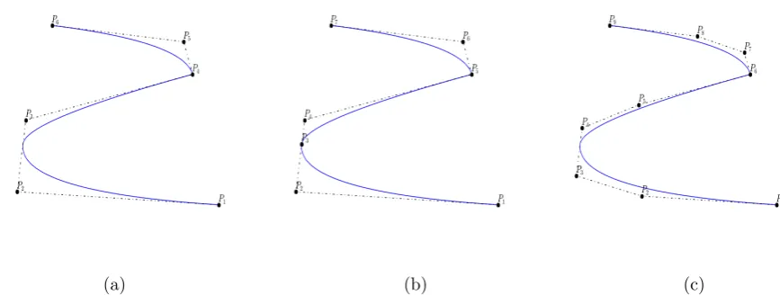
By inserting new knots into the knot vector, we add new control points without changing the shape of the B-Spline curve. This can be done using the DeBoor algorithm [2]. We can also elevate the degree of the B-Spline family and keep unchanged the curve [4]. In (Fig. 2), we apply these algorithms on a quadratic B-Spline curve and we show the position of the new control points.

(a) (b) (c)

Figure 2. (a) A quadratic B-spline curve and its control points. The knot vector isT ={0,0,0,1 2,

3 4,

3 4,1,1,1}.

2.4.

Deriving a B-spline curve

The derivative of a B-spline curve is obtained as:

C0(t) =

n−1 X

i=0

N_ik0(t)Pi= n−1 X

i=0

_p

ti+p−ti

N_ik−1(t)Pi−

p ti+1+p−ti+1

N_ik₊₁−1(t)Pi

=

n−2 X

i=0

N_ik−1∗(t)Qi, (2.3)

whereQi=p_tPi+1−Pi

i+1+p−ti+1, and{N k−1 i

∗

, 0≤i≤n−2}are generated using the knot vectorT∗which is obtained fromT by reducing by one the multiplicity of the first and the last knot (in the case of open knot vector),i.e. by removing the first and the last knot.

More generally, by introducing the B-splines family {N_ik−j∗,0≤i≤n−j−1} generated by the knot vector

Tj∗ obtained fromT by removing the first and the last knotj times, we have the following result:

Proposition 2.6. The jth_{derivative of the curve C is given by}

C(j)_{(t) =} n−j−1

X

i=0

N_ik−j∗(t)P_i(j), where P(_ij)= p−j+ 1

ti+p+1−ti+j

P_i(₊₁j−1)−P_i(j−1) and P(0)_i =Pi,

By denotingC0 andC00the first and second derivative of the B-spline curveC, it is easy to show that:

Proposition 2.7. We have, • C0_{(0) =} p

tp+1(P1−P0),C

00_{(0) =} p(p−1) tp+1

1

tp+1P0− { 1 tp+2+

1

tp+2}P1+ 1 tp+2P2

,

• C0(1) = _1−tp

n−1(Pn−1−Pn−2),C

00_{(1) =} p(p−1) 1−tn−1

1

1−tn−1Pn−1− { 1 1−tn−1 +

1

1−tn−2}Pn−2+ 1

1−tn−2Pn−3

.

2.5.

Multivariate tensor product splines

Let us considerdknot vectorsT ={T1_{, T}2_{,· · · , T}d_{}. For simplicity, we consider that these knot vectors are}

open, which means thatkknots on each side are duplicated so that the spline is interpolating on the boundary, and of bounds 0 and 1. In the sequel we will use the notation I = [0,1]. Each knot vectorTi_{, will generate}

a basis for a Schoenberg space,Ski(T

i_{, I). The tensor product of all these spaces is also a Schoenberg space,}

namelySk(T), wherek={k1,· · · , kd}. The cubeP =Id= [0,1]d, will be referred to as a patch.

The basis forSk(T) is defined by a tensor product:

N_ik:=Nk1 i1 ⊗N

k2

i2 ⊗ · · · ⊗N kd

id,

wherei={i1,· · ·, id}.

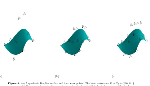
A typical cell fromP is a cube of the form : Qi = [ξi1, ξi1+1]⊗ · · · ⊗[ξid, ξid+1]. In (Fig. 3), we apply knot insertion and elevation degree algorithms on a quadratic B-Spline surface and we show the position of the new control points.

Remark 2.8. A B-splines surface can be converted to a list of B´ezier surfaces. In order to do so, we only need to increase the multiplicity of internal knots to match the spline degree. Therefor, it is easy to extract B´ezier surfaces for all logical elements. Finally, we can elevate their degrees to a desired one.

2.6.

Software implementation

(a) (b) (c)

Figure 3. (a) A quadratic B-spline surface and its control points. The knot vectors areT1=T2={000,111}.

(b) The curve after a h-refinement by inserting the knot{0.5}in both directions, while the degree is kept equal to 2.

(c) The curve after a p-refinement, the degree was raised by 1 (using cubic B-splines).

2.7.

Hermite-B´

ezier finite elements method

We consider a sequence of domains (Ωh) that converges to a 2D domain Ω. We recall that in the case of

the IsoGeometric Analysis approach, we have Ωh= Ω. Let Qh be a partition of Ωh⊂Ω, where every element

e∈ Qh denotes a B´ezier surface. Therefor, an elemente is the image of the unit squareP = [0,1]2 by alocal

mapping, denotedFeand every pointxin the elementecan be written as:

x:=x(s, t) =Fe(s, t) =

p,q

X

i,j=0

xijBie(s)B e

j(t), s, t∈[0,1]. (2.4)

We can then, create a global mapFdefined on every element of the partitionQh as: F|e:=Fe,∀e∈ Qh.

When using B-splines to create B´ezier surfaces, we ensure the global regularity of the mappingFdepending on the knot vectors.

In order to have a standard finite element formulation, we shall use a change of basis to associate the degrees of freedom (i.e. the control points) to the vertices (the 4 summits of the B´ezier surface) of our elements. The new basis is given in Appendix A, Eq. A.34. As we are using the IsoParametric setting, the unknowns are also expressed in the same basis as the positionx.

Remark 2.9. The assembling procedure is done on the logical domain [0,1]2. Therefore, all derivatives are computed on the logical domain and must be transported to the physical domain.

3.

_{Grad-Shafranov solver}

to validate the finite element method in cylindric coordinates. The MHD equilibrium is described by the force balance, the Ampere’s law of the Maxwell equations and the magnetic divergence constraint (Eq. 3.5)



 

 

J×B=∇P, ∇ ×B=µ0J, ∇ ·B= 0.

(3.5)

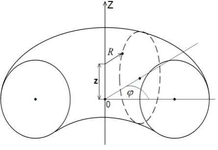
The equilibrium of the plasma in a tokamak (Fig. 4) is assumed axisymmetric and the magnetic fieldBcan be expressed asB=∇ϕ× ∇ψ+g∇ϕwhereϕthe toroidal angle (Fig. 4) andψis the poloidal flux function. The current densityJcan also be written, in the same form, asJ=RJϕ∇ϕ+_µ1₀∇g× ∇ϕ.

Figure 4. The toroidal plasma configuration

UsingB· ∇P = 0 it is easy to see that the pressure is a function of the fluxψ. On the other hand,J· ∇P = 0 implies that the functiong is also a flux function. Inserting these relations in the balance force equation yields to a second order nonlinear elliptic equation, known as Grad-Shafranov-Schl¨uter equation:

∆∗ψ=R∂R

1

R∂Rψ

+∂zz2 ψ=−µ0R2 d dψP−g

d

dψg. (3.6)

The right hand side of the equation (Eq. 3.6) is the input data and is given byg (toroidal magnetic field) and the pressureP =P(ψ).

3.1.

Solver for Grad-Shafranov equation

In the subsection, we are interested in the resolution of the non-linear elliptic partial differential equation:

1

R2∆

∗_ψ:= 1

R∂R ₁

R∂Rψ

+∂2_zzψ=F(R, Z, ψ), on Ω, (3.7)

ψ= 0, on∂Ω. (3.8)

Using a Picard method, we have,

• ψ0 _{is given,}

• knowingψn_{, we solve:}

1

R2∆

∗_ψn+1_{=F(R, Z, ψ}n_{) (3.9)}

The domain Ω will be describe later. Letφ∈ Vh⊂ V a test function withVthe functional space of the solution.

obtain the weak form of the equation :

Z

Ω

1

R∇ψ

n+1_{· ∇φ dΩ =} Z

Ω

F(R, Z, ψn)φ dΩ, ∀φin Vh. (3.10)

We assume thatψn₌PN

j=1ψ n

jφj withN the total of degree of freedom andφj(x) the basis function associated

to thejth_{degree of freedom. By takingφ=φ}

i in the weak form we obtain

N

X

i

ψ_jn Z

Ω

1

R∇φj· ∇φi dΩ

=

Z

Ω

F(R, Z, ψn)φi dΩ ∀i∈ {1, ..N}. (3.11)

At the end solving (Eq. 3.9) is equivalent to solve the linear system

MXn+1=fn, withMij =

Z

Ω

1

R∇φj· ∇φi dΩ

, f_in=

Z

Ω

F(R, Z, ψn)φi dΩ andXn+1=

ψ₁n+1, ...., ψn_N+1 .

3.2.

Numerical results

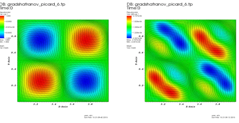
In this section we propose numerical results to validate the finite element method for the Grad-Shafranov equation. A first validation is done for an analytical solution on a square domain. To test in the same time, the mapping we propose to solve the equation on the non Cartesian Collela mesh obtained with the Collela mapping:

x:=η=F(η) = (η1+αsin(k1η1) sin(k2η2), η2+αsin(k1η1) sin(k2η2)). (3.12)

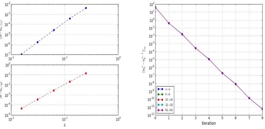
This analytical mapping is approximated by B-Splines surfaces, then we convert them into a collection of cubic B´ezier surfaces. These surfaces are therefor converted into the Hermite-B´ezier form. If the mapping is the identity the mesh is a classical Cartesian mesh. The right hand side and the nonlinear functionF are computed so that the solution vanishes on the boundary, when F contains a quadratic dependence onψ. In figures (Fig 6 and 7) and table (Tab. 1), we show the expected convergence order, while in (Fig. 5), the numerical solution and the numerical error are shown. (Fig. 6) and (Fig. 7) shows also the evolution of the L2 and H1 norms depending on Picard’s iterations. As we may notice, our Picard’s algorithm converges after 6 iterations, but this does not seem to be the rule for other geometries andF functions.

In the sequel, we present different simulations on a realistic geometry (Fig 8) for poloidal plane in the tokamak

L2convergence order

Identity mapping 3.46 3.82 3.95 3.98 Colella’s mapping 3.61 3.15 3.39 3.74

H1_{convergence order}

Identity mapping 2.71 2.90 2.97 2.99 Colella’s mapping 2.38 2.53 2.64 2.85

Table 1. Grad-Shafranov convergence order for the identity and Colella’s mappings: h-dependence of the L2 andH1 norms between the gridsn×nand 2n×2n, withn={4,8,16,32}. For theL2 norm, the values correspond to log2

ku−uHk

ku−uhk withH= 2h. For theH

1

norm, we use the same formulae with the corresponding semi-norm.

Figure 6. L2_andH1 _{errors (left) after convergence (right) and the residual error for each step of the Picard}

algorithm, for the equation (Eq 3.8) on a square domain, using the identity mapping.

based on characteristic parameters describing the cross-section forITER,ASDEX-Upgrade andJET tokamaks. These parameters are: theinverse aspect-ration , theelongation κand thetriangularity δ. They are given by the following formulae :



   

   

R0=Rmin+₂Rmax, =Rmax−R0

R0 =

R0−Rmin

R0 , κ= Zmax

R0 ,

1−δ= R(Z=Zmax)

R0 ,

and



 

 

ψ(Rmax,0) = 0,

ψ(Rmin,0) = 0,

ψ(R(Z =Zmax),±Zmax) = 0.

(3.13)

where in the last equation, we consider a given flux surface (in our case, defined byψ(R, Z) = 0) and R as a function ofZ.

In the following test, we consider the right hand side function

F(R, Z, ψ) =R2, (3.14)

which gives the analytical solution [12],

ψ(R, Z) =R

4

8 +d1+d2R

2_+d

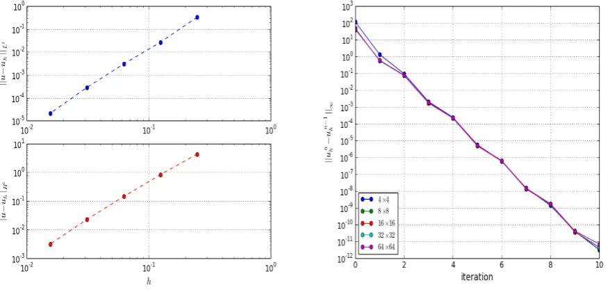
Figure 7. L2_andH1 _{errors (left) after convergence (right) and the residual error for each step of the Picard}

algorithm, for the equation (Eq 3.8) on a square domain, using Collela’s mapping.

Figure 8. Geometric definition of the parameters, κandδ.

Plugging (Eq. 3.13) in (Eq. 3.15) leads to the following system ford1, d2 andd3:





1 (1 +)2 (1 +)4 1 (1−)2 (1−)4

1 (1−δ)2 (1−δ)4−4(1−δ)2κ22 

 

 d1 d2 d3



=−

1 8





(1 +)4 (1−)4 (1−δ)4



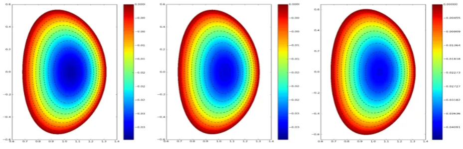
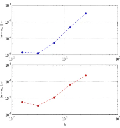
In figure (Fig. 9), we plot the computational domain and the numerical solution for ITER, ASDEX-Upgrade andJET relevant parameters. In (Fig. 11) we plot theL2_andH1_{norms for MESH2 (Fig 10. Meshes generated}

Figure 9. Computational domain in the poloidal plan, in the (R, Z) coordinates, and the analytical solu-tion for: (left) ITER (R0, , κ, δ) = (1,0.32,1.7,0.33), (middle) ASDEX-Upgrade (R0, , κ, δ) =

(1.645,0.311,1.77,0.0932), (right)JET(R0, , κ, δ) = (2.924,0.323,1.87,0.141)

byCAID). In this case, the theoretical convergence order is not achieved; the reason is the bad approximation of the boundary when∂Rψ= 0 or∂Zψ= 0.

Remark 3.1. In order to construct a2D mesh from a given boundary given by an analytical formula, we first need to find a set of points that lie on this boundary. This is done using a Python function. However, we found that the distribution of the given points is not uniform and therefor some parts of the boundary have less points for a B-spline or Hermite reconstruction/interpolation. The loss of the convergence order is related to the bad distribution of these points. This must be fixed in the future in order to allow high order approximation, for arbitray B-spline approximations.

Figure 10. ITERlike relevant parameter domain: (left) MESH1 (right) MESH2.

4.

_{Anisotropic Diffusion}

Figure 11. Convergence order for Iter like relevant parameter domain.

problem in a toroidal geometry. Secondly this problem is singular when the anisotropy of the diffusion tends to the infinity. This singularity leads to an ill-posed problem and generates numerical issues like ill-conditioning and lake of accuracy. In this section, we are interested in the resolution of the anisotropic diffusion problem for both steady and unsteady cases. The anisotropic diffusion time evolution problem is

∂tu=∇ ·(K∇u) +f, x∈Ω, (4.17)

where Ω is the domain,udescribes the temperature inside a tokamak, the conductivityK=κ_kK_k+κIIis a 3

by 3 tensor. The later is a sum of two contributions, first parallel component is given by:

κkKk=κk

BBT

kBk2

for prescribed magnetic field B = ∇ϕ× ∇ψ+g∇ϕ (with ϕ the toroidal angle), κk is a parallel diffusion

coefficient. The second componentκIIis a standard isotropic diffusion. We are interested in highly anisotropic

configurations with κk

κI

'1061.

Circular Plasma For circular cross section plasma, the Grad-Shafranov equation associated to the nonlinear right hand sideF(R, Z, ψ) =R2, leads to

ψ(R, Z) =Cψln

1 +r

2

a2

, with Cψ=

a2

2R0q0

Remark 4.1. When using an analytical equilibrium for anisotropic diffusion or tearing mode problems, the boundary condition for the flux (needed to construct the equilibrium) does not need to be Homogeneous Dirichlet. In fact, in this case, we don’t solve the Grad-Shafranov equation and the flux formula is directly inserted in the conductivity tensor.

General case In the general case, we need to solve the equilibrium (Grad-Shafranov) for the potentialψ

in order to define the magnetic field.

4.1.

The 3D elliptic anisotropic diffusion equation

We start by solving the following anisotropic diffusion problem (Eq. 4.18)

We solve this 3D problem using a tensor product between a 2D circular mesh for the poloidal plan and 1D uniform mesh for the toroidal direction. Let φi be a test function. This 3D function is given as the tensor

product of 2D and 1D basis functions. Multiplying (Eq. 4.18) byφi and integrating by parts leads to

Z

Ω κ_k

kBk2(B· ∇u)(B· ∇φi) +κI∇u· ∇φidΩ = Z

Ω

f φidΩ (4.19)

Using the expansionu=PN

j=1ujφj withN the total number of degrees of freedom, we get

N X j=1 uj Z Ω κk

kBk2(B· ∇φj)(B· ∇φi) +κI∇φj· ∇φi

dΩ =

Z

Ω

f φidΩ, (4.20)

which leads to the linear systemMU=Fwhere

Mij=

Z

Ω κ_k

kBk2(B· ∇φj)(B· ∇φi) +κI∇φj· ∇φidΩ, and Fi= Z

Ω

f φidΩ, ∀i, j∈[1, n]. (4.21)

Remark 4.2. For validation, we take any function u that vanishes on the boundary and then compute f =

−∇ ·K· ∇u. In the case of circular cross section plasma, we takeuexact= 1−(R−R0) 2_+Z2

a2 . For an annulus cross section plasma, an analytical solution is given byuexact=

1−(R−R0)2+Z2 a2

(R−R0)2+Z2 a2

center

−1. It is important to notice that the definition of the conductivity tensor remains the same as well as the relation between the flux

ψ and the magnetic field B. These two analytical solutions are only constructed so that they vanishe on the boundary.

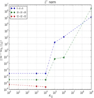
We show in (Fig. 12), the L2 _{error norm for different meshes and values of κ}

k. GMRES was used with a

Jacobi preconditioner for a tolerancetolr= 10−11. Block-Jacobi preconditioner was also tested and results were

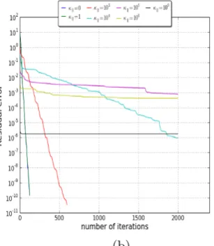
quite equivalent. We may notice that for a diffusion >104 the solver does not converge, because of the bad conditioning of the linear system. This can be viewed in (Fig. 13), where we show the evolution of the residual error for the Krylov solver.

Figure 12. Anisotropic diffusion operator: L2_{error norm depending onκkfor different meshes. The 2D mesh}

is the equivalent of the MESH2 (Fig 10) for a circle. The 1D mesh in toroidal direction is uniform.

4.2.

Time evolution problem

For the time depending problem, we consider the following implicit scheme

un+1−un

∆t − ∇ · K∇u

n+1

(a) (b)

(c)

Figure 13. Anisotropic diffusion operator: evolution of the residual error for the Krylov solver, for a mesh (a) 8×8×8, (b) 16×16×16 and (c) 32×32×32

which leads to

un+1−∆t∇ · K∇un+1=un+ ∆tf. (4.22)

Let φi be a test function. Multiplying (Eq. 4.22) by φi, integrating by parts and using the expansion of

u=Pn

j=1ujφj, leads to the following linear system problem

where fori, j∈[1, n], we have

MI_ij=

Z

Ω

φiφj+ ∆t

_κ

k

kBk2(B· ∇φj)(B· ∇φi) +κI∇φj· ∇φi

dΩ (4.23)

ME

ij=

Z

Ω

φiφjdΩ (4.24)

Fi=

Z

Ω

∆tf φdΩ (4.25)

4.2.1. Transient case

In the sequel, we are interested in the steady state solution of the anisotropic diffusion problem on a circular cross section domain with a mesh type MESH1 and MESH2 (c.f. Fig. 10 for ITER-like relevant parameter domain). In order to avoid the polar-like singularity at the center of the plasma in MESH1, we consider an annulus domain of minimum radius rmin = 0.1, while the maximum radius rmax is kept equal to 1 for both

meshes. The source terms are computed as the solution of the elliptic anisotropic diffusion equation, forκk= 0

with the following analytical solutions







uexact= 1−

(R−R0)2+Z2

a2 , for MESH1,

uexact=

1−(R−R0)2+Z2 a2

(R−R0)2+Z2 a2

center

−1, for MESH2. (4.26)

Numerical simulations were done with time step dt = 5.10−3,1 and a final time Tf inal = 0.5,20 respectively.

GMRES and Jacobi preconditioner were used. In (Fig. 14,16), we show the finalL2andH1norms as functions ofκ_kfor different meshes while in (Fig. 15, 17), we show the time evolution of theL2_andH1_{norms. Finally, in}

table (2), we show the power approximation, h-dependance, of theL2_andH1_{norms between the grids 8×4×4}

and 16×8×8. As we can notice, the convergence order is conserved at the final time.

As seen in the convergence study of the Hermite-B´ezier elements (table 2), when increasing the grid points, the value of the numerical convergence order achieved between 2 consecutive grids tends to the theoretical value 4. Therefor finer grids should lead to a better numerical convergence order.

Figure 14. Short time behavior ofL2_andH1 _{error norms for different values ofκkat timeT}

f inal= 0.5 and

Figure 15. Short time behavior of L2 _{and H}1 _{error norms evolution for the transient anisotropic diffusion}

using MESH1 fordt= 5.10−3_{and a grid 16×8×8.}

Figure 16. Long time behavior ofL2 _andH1_{error norms for different values ofκkat timeT}

f inal= 20 and

dt= 1 using MESH2.

4.2.2. Evolution of a Gaussian Pulse

Figure 17. Long time behavior of (first line)L2 and (second line)H1error norms evolution for the transient anisotropic diffusion using MESH2 for anddt= 1 and a grid (left) 16×8×6 and (right) 32×16×6.

κ 0 1 103 104 105 106

L2_norm

Initial time (t= 0) 3.675 3.675 3.684 3.689 3.69 3.68 Final time (t= 0.5) 3.544 3.544 3.55 3.55 3.55 3.544

H1norm

Initial time (t= 0) 2.925 2.925 2.918 2.911 2.907 2.906 Final time (t= 0.5) 2.865 2.865 2.858 2.85 2.845 2.843

Table 2. Transient state h-dependence of the L2 _{and H}1 _{norms between the grids 8×4×4 and} 16×8×8. For theL2 _{norm, the values correspond to log}

2

ku−uHk

ku−uhk withH= 2h, evaluated

at t= 0 andt= 0.5. For theH1 _{norm, we use the same formulae with the corresponding} semi-norm.

with a diffusion in the direction of the magnetic field. The initial data is given by

u(t= 0,x) =e−σ12((R−R1)2−R21ϕ2−Z2)_{, (4.27)}

where R1 = 3.5, σ = 0.1, κI = 0 and κk = 1. In this case, energy on any given toroidal surface should be

conserved. In order to validate our simulation, we compute and plot the mean value of the numerical solution on a toroidal surface

¯

u(t, R) =

Z 2π

0 Z 2π

0

Ru dϕdθ (4.28)

Figure 18. Meshes. in the top the non aligned mesh (NAM) with 32×32 and 64×64 cells. In the bottom the perturbed aligned mesh (PAM) with 32×64 cells and the aligned mesh with 32×32 cells.

in the perpendicular direction but then solutions in not good (the diffusion is slower and not at the right place). Consequently, the mesh can affect the tensor of diffusion coefficient.

4.3.

Future work

In this work, we focused on the development of a finite element method based on Hermite-Be´ezier surfaces. The code is written in Fortran, using MPI for parallelization. A new feature of the code is the ability to create any finite element space using a linear expansion over Bernstein polynomials on quadrangles and triangles. The code is still in an early stage and further optimization are beeing studied and will be implemented. A Computer Aided Designe tool has been also developed that allows us to create and manipulate the geometry easily. For instance, one can convert the Hermite-B´ezier description into a B-spline one and reciprocally. A new implementation of the resolution ofψ(R, Z) = 0 must be done in order to fit accurately the boundary.

In a future work, we will derive the h-estimators for the Hermite-B´ezier elements. We also need to derive some mesh-quality estimators based on anisotropic estimations. This will allows us for instance to see the impact of the geometry in anisotropic diffusion problem. This quantitative study has never been done and we need to provide a suffiient mathematical framework for the Hermite-B´ezier elements.

Finally, as a continuation of this work, we will study a tearing mode and compare different kind of discretiza-tions in a future work.

5.

Conclusions

We have developed a finite element method based on Hermite-B´ezier elements for the poloidal plane (quad-rangular elements) and a toroidal geometry (hexahedral elements). In order to create the partition of the computation domain Ω into B´ezier surfaces, we use B-Spline surfaces, which allows us to control the regularity between elements and when needed (if possible), aC1 _{regularity can be imposed. Numerical results are shown}

Figure 19. u(t, R) for the time¯ t= 20. in the top the non aligned mesh (NAM) with 32×32 and 64×64 cells. In the bottom the perturbed aligned mesh (PAM) with 32×64 cells and the aligned mesh with 32×32 cells.

to the bad approximation of the boundary. This point will be treated in a future work. Secondly, we apply our finite element method to the resolution of an anisotropic diffusion problem, where we have observed the usual asymptotic error for very strong anisotropy. Future work will focus on this behavior to improve the accuracy either by meshes alignment or by asymptotic preserving preconditioning.

Acknowledgement. We warmly thank the referees for their useful comments and remarks, which helped us to improve the quality of this work.

References

[1] Orain F. B´ecoulet M. and al. Mechanism of edge localized mode mitigation by resonant magnetic perturbations.Phys. Rev. Lett., 113:115001, Sep 2014.

[2] C. DeBoor.A practical guide to splines. Springer-Verlag, New York, applied mathematical sciences 27 edition, 2001. [3] R. T. Farouki and V. T. Rajan. On the numerical condition of polynomials in Berstein form. Comput. Aided Geom. Des.,

4(3):191–216, November 1987.

[4] Qi-Xing Huang, Shi-Min Hu, and Ralph R. Martin. Fast degree elevation and knot insertion for B-spline curves. Computer Aided Geometric Design, 22(2):183 – 197, 2005.

[5] G. T. A. Huysmans, S. Pamela, E. Van Der Plas, and P. Ramet. Non-linear MHD simulations of edge localized modes (ELMs). Plasma Physics and Controlled Fusion, 51(12):124012, 2009.

[6] G.T.A. Huysmans and O. Czarny. MHD stability in X-point geometry: simulation of ELMs.Nuclear Fusion, 47(7):659, 2007. [7] G.T.A. Huysmans and A. Loarte. Non-linear MHD simulation of ELM energy deposition.Nuclear Fusion, 53(12):123023, 2013. [8] W. Tiller L. Piegl.The NURBS Book. Springer-Verlag, Berlin, Heidelberg, 1995. second ed.

[9] A. Mentrelli and C. Negulescu. Asymptotic-preserving scheme for highly anisotropic non-linear diffusion equations.J. Comput. Physics, 231(24):8229–8245, 2012.

Figure 20. u(t, R) for the time¯ t= 60. in the top the non aligned mesh (NAM) with 32×32 and 64×64 cells. In the bottom the perturbed aligned mesh (PAM) with 32×64 cells and the aligned mesh with 32×32 cells.

[11] F. Orain, M. B´ecoulet, G. Dif-Pradalier, G. Huijsmans, S. Pamela, E. Nardon, C. Passeron, G. Latu, V. Grandgirard, A. Fil, A. Ratnani, I. Chapman, A. Kirk, A. Thornton, M. Hoelzl, and Cahyna P. Non-linear magnetohydrodynamic modeling of plasma response to resonant magnetic perturbations.Physics of Plasmas (1994-present), 20(10), 2013.

[12] A. Pataki, A. J. Cerfon, J. P. Freidberg, L. Greengard, and M. O Neil. A fast, high-order solver for the Grad-Shafranov equation.Journal of Computational Physics, 243(0):28 – 45, 2013.

[13] A. Ratnani. Caid : Computer aided isogeometric design tool using python. https://github.com/ratnania/caid/tree/devel. [14] A. Ratnani. Python for isogeometric analysis. https://github.com/ratnania/pigasus/tree/devel.

A.

_{Appendix A:}

Let us consider a cubic B´ezier patch

x(s, t) = 3

X

i,j=0

xijBi(s)Bj(t), s, t∈[0,1] (A.29)

Computing derivatives of this surface on the four (logical) points{(s, t) = (0,0),(0,1),(1,0),(1,1)}leads to

    

   

x(0,0) =x00, xs(0,0) = 3(x10−x00), xt(0,0) = 3(x01−x00), xst(0,0) = 9(x00+x11−x01−x10)

x(0,1) =x03, xs(0,1) = 3(x13−x03), xt(0,1) = 3(x03−x02), xst(0,1) = 9(x03+x12−x02−x13)

x(1,0) =x30, xs(1,0) = 3(x30−x20), xt(1,0) = 3(x31−x30), xst(1,0) = 9(x30+x21−x20−x31)

x(1,1) =x33, xs(1,1) = 3(x33−x23), xt(1,1) = 3(x33−x32), xst(1,1) = 9(x33+x22−x23−x32)

Figure 21. u(t, R) for the time¯ t= 100. in the top the non aligned mesh (NAM) with 32×32 and 64×64 cells. In the bottom the perturbed aligned mesh (PAM) with 32×64 cells and the aligned mesh with 32×32 cells.

Now, let us introduce the following quantities

     

    

a00=kx10−x00k, b00=kx01−x00k, u00= x10_a−x00

00 , v00= x01−x00

b00 , w00=

x00+x11−x01−x10 a00b00 a03=kx13−x03k, b03=kx03−x02k, u03= x13_a−x03

03 , v03= x03−x02

b03 , w03=

x03+x12−x02−x13 a03b03 a30=kx30−x20k, b30=kx31−x30k, u30= x30_a−x20

30 , v30= x31−x30

b30 , w30=

x30+x21−x20−x31 a30b30 a33=kx33−x23k, b33=kx33−x32k, u33= x33_a−x23

33 , v33= x33−x32

b33 , w33=

x33+x22−x23−x32 a33b33

(A.31)

Therefore, our B´ezier patch can be rewritten as

x(s, t) =x00M00(s, t) +a00u00N01(s, t) +b00v00P02(s, t) +a00b00w00Q03(s, t)

+x03M10(s, t) +a03u03N11(s, t) +b03v03P12(s, t) +a03b03w03Q13(s, t)

+x30M30(s, t) +a30u30N30(s, t) +b30v30P30(s, t) +a30b30w30Q30(s, t)

+x33M33(s, t) +a33u33N33(s, t) +b33v33P33(s, t) +a33b33w33Q33(s, t) (A.32)

But, since

    

   

x10=a00u00+x00, x01=b00v00+x00, x11=a00b00w00+a00u00+b00v00+x00

x13=a03u03+x03, x02=−b03v03+x03, x12=a03b03w03+a03u03−b03v03+x03

x20=−a30u30+x30, x31=b30v30+x30, x21=a30b30w30−a30u30+b30v30+x30

x23=−a33u33+x33, x32=−b33v33+x33, x22=a33b33w33−a33u33−b33v33+x33

Now plugging these relations into (Eq. A.29), we get

x(s, t) =x00M00(s, t) +a00u00N01(s, t) +b00v00P02(s, t) +a00b00w00Q03(s, t)

+x03M10(s, t) +a03u03N11(s, t) +b03v03P12(s, t) +a03b03w03Q13(s, t)

+x30M30(s, t) +a30u30N30(s, t) +b30v30P30(s, t) +a30b30w30Q30(s, t)

+x33M33(s, t) +a33u33N33(s, t) +b33v33P33(s, t) +a33b33w33Q33(s, t) (A.34)

where the new basis is (Eq. A.35)

               

               (

M00(s, t) =B0(s)B0(t) +B1(s)B0(t) +B0(s)B1(t) +B1(s)B1(t), N00(s, t) =B1(s)B0(t) +B1(s)B1(t) P00(s, t) =B0(s)B1(t) +B1(s)B1(t), Q00(s, t) =B1(s)B1(t)

(

M03(s, t) =B0(s)B3(t) +B1(s)B3(t) +B0(s)B2(t) +B1(s)B2(t), N03(s, t) =B1(s)B3(t) +B1(s)B2(t) P03(s, t) =−B0(s)B2(t)−B1(s)B2(t), Q03(s, t) =B1(s)B2(t)

(

M30(s, t) =B3(s)B0(t) +B2(s)B0(t) +B3(s)B1(t) +B2(s)B1(t), N30(s, t) =−B2(s)B0(t)−B2(s)B1(t) P30(s, t) =B3(s)B1(t) +B2(s)B1(t), Q30(s, t) =B2(s)B1(t)

(

M33(s, t) =B3(s)B3(t) +B2(s)B3(t) +B3(s)B2(t) +B2(s)B2(t), N33(s, t) =−B2(s)B3(t)−B2(s)B2(t) P33(s, t) =−B3(s)B2(t)−B2(s)B2(t), Q33(s, t) =B2(s)B2(t)

(A.35)