Diffusion approximation in a radiative transfer model for astrophysical flows

Laurence CARASSUS, Marion DARBAS, Ghislaine GAYRAUD, Olivier GOUBET, St´ephanie SALMON

DIFFUSION APPROXIMATION IN A RADIATIVE TRANSFER MODEL FOR

ASTROPHYSICAL FLOWS

Laurent Di Menza

, Claire Michaut

and Oc´

eane Saincir

Abstract. In this work, we present the diffusion approximation model for radiative transfer when we deal with optically thick astrophysical flows. Since the initial model is high CPU time demanding when dealing with its numerical approximation, solving this simpler system can provide a low cost strategy for the simulation of radiative media. We then use a finite-volume algorithm coupled with an implicit scheme for radiative contributions to solve this simplified system. Numerical experiments in the one-dimensional and two dimensional cases are presented to validate our numerical strategy and to prove the relevance of this asymptotic model.

R´esum´e. Nous pr´esentons dans ce travail un mod`ele du r´egime de la diffusion pour le transfert radiatif dans le cas o`u le milieu est optiquement tr`es ´epais pour la description d’´ecoulements astrophysiques. Ce mod`ele permet d’envisager des strat´egies num´eriques moins coˆuteuses en temps que le mod`ele M1 pour la simulation de processus radiatifs. Nous utilisons pour cela une m´ethode de type volumes finis coupl´ee `a un sch´ema implicite pour les termes de rayonnement et nous pr´esentons des r´esultats de simulations num´eriques en dimension 1 et 2 d’espace permettant de valider notre algorithme et de montrer la pertinence de ce mod`ele.

1.

Introduction

The comprehension of realistic astrophysical phenomena has been the subject of many challenging studies for decades, with various applications in stellar physics such as the study of jets in the formation of young stars involving matter accretion, stellar winds and dynamics of supernova remnants. Within this framework, a wide complexity occurs for different reasons. First, these phenomena involve both hydrodynamics and radiative processes (see [16], [18], [25]). The latter ones are driven by the propagation of photons at the speed of light, which means that typical velocities completely differ between hydrodynamic and radiation scales. This causes a strong coupling between fluid and radiation since the behavior of the medium at a given point may depend on quantities which need to be evaluated on a large spatial zone (the physical effects are said to benonlocal). Moreover, in the general case the analytical expression for the physical values under study is out of reach due to the complexity of the governing model. In this case, one can use numerical methods in order to simulate the physical phenomena as accurately as possible. Consequently, mathematical algorithms that are involved have to be consistent with the desired solutions (see [21]). In particular, they have to tolerate discontinuities that may spatially propagate (known as ”shock waves”) and they have to produce physically relevant results (namely

1 _{LMR, FRE CNRS 2011, Universit´e de Reims Champagne-Ardenne, Moulin de la Housse, 51687 Reims Cedex 2 France and}

LUTH, Observatoire de Paris, PSL Research University, CNRS, Universit´e Paris Diderot, 92190 Meudon, France

2 _{LUTH, Observatoire de Paris, PSL Research University, CNRS, Universit´e Paris Diderot, 92190 Meudon, France}

3 _{LMR, FRE CNRS 2011, Universit´e de Reims Champagne-Ardenne, Moulin de la Housse, 51687 Reims Cedex 2 France and}

LUTH, Observatoire de Paris, PSL Research University, CNRS, Universit´e Paris Diderot, 92190 Meudon, France c

EDP Sciences, SMAI 2018

entropic solutions). Finally, one has to implement robust methods in order to handle extreme ratios that may be encountered for typical quantities such as density, pressure, radiative energy, time and space scales.

In this paper, we deal with an asymptotic model for the radiative transfer known as the diffusion approxi-mation for which the mean free path of photons is assumed to be small in terms of the characteristic length. In this case, radiative effects are considered as local, leading to a simplified model which has been the subject of various studies in the last decade (see [2], [3], [9], [16], [23], [26]). We then propose a numerical strategy based on finite volume methods that are widely used for the resolution of hyperbolic problems, with an implicit coupling between hydrodynamics and radiative processes.

This paper is organized as follows: in Section 2, the physical model is discussed, with a focus on the diffusion approximation. In Section 3, the numerical method used for the computation of approximate solution is detailed. Some numerical results obtained in dimensions 1 and 2 are presented in Section 4. Finally, discussion and perspectives are addressed in Section 5.

2.

_{Physical model}

We first intend to present the general physical model for radiative transfer as well as the optically thick approximation leading to the diffusion approximation.

2.1.

Pure hydrodynamic model

We here recall the classical hydrodynamic description of a given gas where we look for the time evolution of the physical quantities such as densityρ, pressurep, velocity field u = (u, v)T _{and total energy E per volume}

unit, that will be assumed to depend on timet and spacex. From the conservation of mass, momentum and total energy, the governing model is the classical Euler system

∂tρ+∇ ·(ρu) = 0

∂t(ρu) +∇ ·(ρ(u⊗u) +pI) = 0

∂tE+∇ ·(u(E+p)) = 0.

(1)

In order to get a closed system, one needs the equation of state that enables to evaluate the pressure in terms of the hydrodynamic quantities. For ideal gases, one has

p= (γ−1)E−1 2ρkuk

2

,

whereγ stands for the adiabatic index (for diatomic gas,γ= 1.4). Note that it is possible to express the total energy with respect to the temperatureT as

E=ρcvT+

1 2ρkuk

2_{, (2)}

where cv denotes the heat capacity at constant volume. System (1) has been intensively studied both from

a mathematical and numerical point of view. It is well-known to belong to the class of hyperbolic systems requiring to use numerical methods capable to compute discontinuous states as well as entropic solutions.

2.2.

Radiative model

having specific intensity I =I(t, x;n, ν), propagating alongn into solid angle dΩ in frequency band dν in an interval time dtremoves an amount of energy

δE=χ(t, x;n, ν)I(t, x;n, ν) dldSdΩ dνdt.

From χ, one can define the mean free path of photons λ = (1/χ) expressed in cm. Moreover, we break the extinction coefficient into a true absorption coefficient κ(t, x;n, ν) and a scattering coefficientσ(t, x;n, ν) such that

χ(t, x;n, ν) =κ(t, x;n, ν) +σ(t, x;n, ν).

The emission coefficient η(t, x;n, ν) of the material is defined such that the amount of energy released by a material element of length dl and cross section dS propagating along ninto solid angle dΩ in frequency band dν in an interval time dt is

δE0=η(t, x;n, ν) dldSdΩ dνdt.

In the same way,η can be separated into a thermal partηt_{and a scattering partη}s _{such that}

η(t, x;n, ν) =ηt(t, x;n, ν) +ηs(t, x;n, ν).

The transfer equation is obtained computing the difference between the amount of energy between positionx andx+ ∆xand timetandt+ ∆twhich equals the difference between the amount of energy created by emission and the amount absorbed by the material. Consequently, one has

I(t+ ∆t, x+ ∆x;n, ν)−I(t, x;n, ν)dSdtdΩ dν =η(t, x;n, ν)−χ(t, x;n, ν)I(t, x;n, ν)dldSdtdΩ dν.

Setting ∆t= dl/c, thus we have

I(t+ ∆t, x+ ∆x;n, ν) =I(t, x;n, ν) + ₁

c ∂I ∂t +

∂I ∂l

dl.

Moreover, in cartesian coordinates, ∂I_∂l =n· ∇I wherenis the unit vector along the direction of propagation. The transfer equation is then

₁

c ∂

∂t +n· ∇

I(t, x;n, ν) =η(t, x;n, ν)−χ(t, x;n, ν)I(t, x;n, ν). (3)

From the intensityIevaluated at a given frequencyν, it is possible to define radiative energyE, radiative flux F and radiative pressureP as the first moments ofI, that is

E(t, x;ν) = 1 c

Z

S2

I(t, x;n, ν) dΩ,

F(t, x;ν) = Z

S2

I(t, x;n, ν)ndΩ,

P(t, x;ν) = 1 c

Z

S2

I(t, x;n, ν) (n⊗n) dΩ.

From these expressions, we compute the total radiative quantities integrating all the elementary contributions over all frequencies

ER(t, x) =

Z +∞

0

E(t, x;ν) dν, FR(t, x) =

Z +∞

0

F(t, x;ν) dν, PR(t, x) =

Z +∞

0

Integrating the transport equation (3) for all possible frequencies and directions, one gets

∂tER+∇ ·FR=

Z +∞

0 Z

S2

η(t, x;n, ν)−χ(t, x;n, ν)I(t, x;n, ν)dΩ dν:=−cG0.

Similarly, it is possible to derive the equation of radiative momentum as

1

c2∂tFR+∇ ·PR= 1 c

Z +∞

0 Z

S2

η(t, x;n, ν)−χ(t, x;n, ν)I(t, x;n, ν)ndΩ dν :=−G.

At local thermal equilibrium, the source terms arising in these equations can be expressed in the frame where particles are always at rest, the comoving frame (with subscript ”0”), asG0=κEER,0−κPaRT4,G=κFFR,0/c, involving the first radiative constant aR, the gas temperatureT and Planck, energy and flux mean opacities

defined by

κP =

R+∞

0 κ(ν)B(ν, T) dν R+∞

0 B(ν, T) dν

, (4)

κE=

R+∞

0 κ(ν)E(ν) dν R+∞

0 E(ν) dν

, (5)

κF =

R+∞

0 κ(ν)F(ν) dν R+∞

0 F(ν) dν

, (6)

where B(ν, T) is the Planck function. To simplify (G0_{, G), we assume that the radiation has a blackbody} spectrum which means that E(ν) ∝ B(ν, T), leading to κE = κP. In order to close the system, we use the

relationPR=DER where the Eddington tensor (see [11]) is given by

D= 1−χ¯ 2 I+

3 ¯χ−1 2

f⊗f

kfk2

involvingf = FR

cER. The Eddington factor ¯χis obtained by minimizing the radiative entropy (see [4], [17]) and writes

¯

χ= 3 + 4kfk 2

5 + 2p4−3kfk2.

One obtains with this closure relationship the so-called M1 model for the description of the radiative transfer. Finally, one gets the system of radiation hydrodynamics by coupling this model with the Euler system

∂tρ+∇ ·(ρu) = 0

∂t(ρu) +∇ ·(ρ(u⊗u) +pI) =G

∂tE+∇ ·(u (E+p)) =c G0

∂tER+∇ ·FR =−c G0

∂t c−2FR+∇ ·PR =−G.

(7)

of radiation hydrodynamics, HADES code based on the M1 model has been developed in LUTH (see [13]). In the following section, we introduce an asymptotic regime leading to numerical routines used in HADES within the framework of local radiative effects.

2.3.

Diffusion approximation

It is well-known that two extremal regimes can be observed in radiative transfer, leading to simplified models depending on the ratio between the mean free path λof photons and the characteristic length L of the phe-nomenon under study. The first one is known as theoptically thincase for whichλL. It is then possible to derive an Euler system involving a cooling function as a source term in the equation of the energy conservation. In the second one referred as the optically thick case, we assume that λ L. Radiative effects are assumed to be local since emitted photons are absorbed almost instantaneously and do not come into play outside the considered spatial point. In this specific case, the radiative flux FR in the comoving frame expresses as

FR,0=− 1 3

c κR

∇ER,0

whereκR is the Rosseland mean opacity defined by

κ−1_R = R+∞

0 χ

−1_(ν)∂

TB(ν, T) dν

R+∞

0 ∂TB(ν, T) dν

.

Since the radiation field is assumed to be isotropic, the radiative pressure rewritesPR,0= 1₃ER,0I. Moreover, as c−1_F

R=O(λ/L) in terms ofER and PR, we can neglect the time derivative ∂t(c−2FR). Keeping all terms up

toO(u/c) and dropping at least some terms that are of order O (u/c)2

in the streaming limit and the static and diffusion limits, one obtains the new system of radiation hydrodynamics in the diffusion approximation where radiative quantities are expressed in the comoving frame (see [9]) as

∂tρ+∇ ·(ρu) = 0

∂t(ρu) +∇ ·(ρ(u⊗u) +pI) = −

1 3∇ER

∂tE+∇ ·(u(E+p)) = cκP(ER−aRT4) +

1

3u· ∇ER

∂tER+∇ ·

4

3uER

= ∇ ·

_c

3κR

∇ER

−cκP(ER−aRT4)−

1

3u· ∇ER.

(8)

where we have removed the subscript ”0”.

3.

Numerical method

We now aim to solve numerically Syst. (8). For hydrodynamics, great efforts have been paid in order to derive robust numerical methods especially designed to tolerate discontinuities and high Mach numbers. We write (8) under the general form

∂U

∂t +∇ ·F(U) =S(U), (9)

with

U = (ρ, ρu, E, ER) T

, F(U) =

ρu, ρ(u⊗u) +p_I,u (E+p),4 3uER

T

and

S(U) =

0,−1

3∇ER, cκP ER−aRT

4₊1

3u· ∇ER, 1 3

c κR

∆ER−cκP ER−aRT4−

1

3u· ∇ER T

We perform our computations on a cartesian bidimensional uniform spatial grid. Considering a time discretiza-tion with a prescribed time step δt, we then globally split the resolution of Eq. (9) using Strang algorithm (see [20]) to treat alternatively the homogeneous part and the nonhomogenous part at each time increment. Let us mention that S(U) involves divergence terms since when considering the full first-order contribution, the eigenvalues of the Jacobian matrix cannot be easily calculated, which makes the numerical resolution quite delicate.

3.1.

Homogeneous part

Setting S(U) = 0 in (9), we deal with the hyperbolic system

∂U

∂t +∇ ·F(U) = 0. (10)

We use a Strang splitting to solve (10) separately inxandydirections and we perform a finite volume approach. Defining respectivelyδtandδxas the time step and the space step, and notingtn=nδtandxj±1/2= (j±1/2)δx, we calculate the average valueU_jn of the solution of (10) at timetn and over the cellIj= [xj−1/2, xj+1/2]. For this aim, we use the MUSCL-Hancock scheme (see [24]) which is second-order accurate in time and space. The evaluation of numerical fluxes requires to compute the solution of the Riemann problem, that is from an initial data consisting in two constant states separated by an initial discontinuity, for linearized equations. We then use HLLC solver (see [22]) to compute the flux Fhllc _{between each interfacex}

j+1

2 for which we add the new component forER. The classical form of the finite volume scheme expresses as

1 δt(U

n+1

j −U n j) +

1 δx

Fhllc(U_jn, U_jn₊₁)−Fhllc(U_jn₋₁, U_jn)= 0

where the boundary flux at the interface separating constant states UL = (ρL, ρLuL, ρLvL, EL, ER,L) and UR= (ρR, ρRuR, ρRvR, ER, ER,R) writes

Fhllc(UL, UR) =



   

   

F(UL) if 0≤SL

F∗L =F(UL) +SL(U∗L−UL) ifSL<0≤S∗

F∗R=F(UR) +SR(U∗R−UR) ifS∗<0≤SR

F(UR) ifSR<0

. (11)

In (11),SL,S∗ andSR are the wave speeds corresponding respectively to the eigenvaluesu−c,uandu+cof

the system. Moreover, the two intermediate statesU∗L andU∗R are given by

U∗L= 

      

ρL(SL−uL)/(SL−u∗)

ρLu∗(SL−uL)/(SL−u∗)

ρLvL(SL−uL)/(SL−u∗)

EL+ρLu∗(u∗−uL) +

u_∗−u_L

SL−uL

pL

(SL−uL)/(SL−u∗)

(SL−4/3uL)/(SL−4/3u∗)ER,L



      

(12)

and

U∗R = 

      

ρR(SR−uR)/(SR−u∗)

ρRu∗(SR−uR)/(SR−u∗)

ρRvR(SR−uR)/(SR−u∗)

ER+ρRu∗(u∗−uR) +

u_∗−u_R

SR−uR

pR

(SR−uR)/(SR−u∗)

(SR−4/3uR)/(SR−4/3u∗)ER,R



      

where u∗ =S∗. For both intermediate statesU∗L andU∗R, the fifth components are obtained using Rankine-Hugoniot jump conditions (see [8], [19]) as for classical Euler equations with HLL type Riemann solvers.

3.2.

Nonhomogeneous part

We now deal with the reduced system

              

∂t(ρu) = −

1 3∇ER

∂tE = cκP(ER−aRT4) +

1

3u· ∇ER

∂tER = ∇ ·

_c

3κR

∇ER

−cκP(ER−aRT4)−

1

3u· ∇ER

that is treated using a fully time implicit discretization, from the stateUn = (ρn,(ρu)n,(ρv)n, En, E_Rn)T result-ing from the previous step. Since the first component of the total system is left unchanged, we haveρn+1=ρn. Furthermore, we choose to use (2) to compute the total energy. In such a way, we obtain an implicit system in whichu,T andER are sought at timetn+1. Since we perform a dimensional splitting, we here describe our

algorithm when onlyxderivative operators are considered. The time discretized system writes

                 ρn δt u

n+1_−un +1

3∂xE

n+1

R = 0

1 δt

ρncv(Tn+1−Tn) + ρn

2 (u

n+1₎2

−(un)2= cκP 2

E_Rn+1−aR(Tn+1)4

+1

3u

n+1_∂

xERn+1

1 δt E

n+1

R −E n R

=∂x

c 3κn

R

∂xEnR+1

−cκP

2

En_R+1−aR(Tn+1)4

−1

3u

n+1_∂

xEnR+1.

(14)

In (14), the unknown quantities continuously depend on spatial location (x, y). Since this is a fully nonlinear system due to kinetic and thermal contributions, we seek a linearly implicit approximation of the nonlinear terms. First, we have

(un+1)2= (un+un+1−un)2= (un)2

1 +u

n+1_−un

un

2

' −(un)2+ 2unun+1

dropping off the quadratic contribution inun+1_−un_{. Similarly, one finds that (T}n+1₎4_{' −3(T}n₎4_+4(Tn₎3_Tn+1 and plugging these expressions into (14) gives a simplified system that turns out to be linear inun+1,Tn+1and E_Rn+1. After some computations, we find thatER solves

"

1+cκPδt 2 −∂x

cδt 3κn R

∂x

+

un_δt 3 −

2δt2

9ρn∂xE n R

∂x− 2cκPaRδt(T

n₎3

ρn_cv

δt + 2aRcκP(Tn)3

2un 3 −

2δt 9ρn∂xE

n R

∂x+cκP 2

#

ERn+1

=ERn− 3

2aRcκPδt(T n

)4− δt 2

9ρn(∂xE n R)

2

+ 2cκPaRδt(T n₎3

ρn_cv

δt + 2aRcκP(Tn)3

ρn_cv δt T

n +3

2aRcκP(T n

)4+ δt 9ρn(∂xE

n R)

2

(15)

that takes the general formM E_Rn+1=f. Once this linear equation is solved, it is possible to computeun+1 _as

un+1_=un₋ δt

3ρn∂xERn+1 andT

n+1 _{as the solution of the linear equation}

_ρn_c v

δt + 2aRcκP(T n₎3

Tn+1= _2un

3 − 2δt 9ρn∂xE

n R

∂x+ cκP

2

En_R+1+ρ

n_c v δt T

n₊3

2aRcκP(T

n₎4₊ δt 9ρn(∂xE

n R)

involving a diagonal matrix. We finally update the value of total energy En+1 _{as E}n+1 _{= ρ}n_c

vTn+1 +

1 2ρ

n_(un+1₎2_{. We now spatially discretize the two operators∂}

x

cδt

3κn R

∂x

andβn_∂

xin (15) on the one-dimensional

uniform gridx1, . . . , xN. The first one is approximated atxi using the formula

∂x

_cδt

3κn R

∂xfn+1

i ≈cδt 3 ₁ κR

i+1 2

f_in₊₁+1−f_in+1

δx2 −

₁

κR

i−1 2

f_in+1−f_in₋₁+1 δx2

!

where (κR)i+1

2 =

(κR)i+1+(κR)i

2 and (κR)i−1

2 =

(κR)i+(κR)i−1

2 . The second one is discretized using

(βn∂xfn+1)i≈

1 2β

n i

f_in₊₁+1−f_in₋₁+1

δx −

1 2|β

n i|

f_in₊₁+1−2f_in+1+f_in₋₁+1 δx

that enables to mimic the propagation across characteristic curves of the transport operator β∂x for any sign

of the speed. Consequently, we express βn_∂ xas

(βn∂x)fn+1=

1 2δx              

0 βn

1 . . . 0

−βn₂ 0 β₂n

. ._. . ._. . ._. 0 . . . −β_Nn 0

       +       

2|βn

1| −|β1n| . . . 0 −|β₂n| 2|β₂n| −|β₂n|

. ._. . ._. . ._. 0 . . . −|β_Nn| 2|β_Nn|

                    

f₁n+1

.. .

f_Nn+1

       .

Taking the complete two-dimensional case, we would obtain pentadiagonal contributions that require more computational efforts for the numerical implementation. This explains the reason why we performed an alternate direction splitting that consists of one-dimensional iterative resolutions. Since the system that has to be inverted is tridiagonal but not symmetric, we use a LU decomposition algorithm. Once again, the second-order Strang strategy is used, giving a good compromise between computational efficiency and numerical accuracy.

4.

Numerical results

In this Section, we present various numerical simulations that have been performed in order to validate our numerical code. We first present a shock-tube test in the context of radiative flows in strong equilibrium regime, that appears as a generalization of the usual hydrodynamic benchmark test. We then focus on a radiative shock raised by a left-sided piston. We also simulate subcritical and supercritical shocks and finally present two-dimensional simulations, the first one in a radial geometry and the second one with an initial data constant on four quadrants.

4.1.

Shock-tube test

We begin with a test that has been presented in [26]. This is a purely one-dimensional test for an ideal gas with adiabatic indexγ= 5/3 and mean molecular weightµ= 1 in the relationship between the pressure and the temperaturep=ρkBT /(µmH) wherekBis the Boltzmann contant andmHthe hydrogen mass. A discontinuity

initially separates two constant states with the following values: ρL= 10−2kg m−3,TL= 1.5×106K,uL= 0

m s−1andρR= 10−2 kg m−3,TR= 3×105 K,uR= 0 m s−1. Consequently, the initial density is uniform and

the contrast between left and right temperatures is 5. In this test, it is assumed an initial thermal equilibrium in the gas, which means that Er=aRT4. We impose constant opacities set toκP = 108 m−1 and κR = 1010

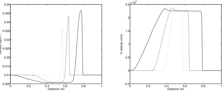
m−1_{. In this regime, radiative pressure cannot be neglected. We plot in Figures 1 and 2 profiles of density,} velocity, total pressure p+Prad and radiative energy that have been computed with the following numerical

0 0.2 0.4 0.6 0.8 1 0.005

0.01 0.015 0.02 0.025 0.03 0.035 0.04 0.045 0.05

Distance (m)

Density (kg/m

3)

0 0.2 0.4 0.6 0.8 1

−0.5 0 0.5 1 1.5 2 2.5x 10

5

Distance (m)

X velocity (m/s)

Figure 1. Snapshots of the solution at different times (t= 2.5×10−7 s, 5×10−7 s, 10−6s).

Left: density profile versusx. Right: velocity profile versusx.

conditions involving ghost cells have been prescribed at each extremity of the spatial domain, in order to avoid spurious reflexions caused by the boundaries.

0 0.2 0.4 0.6 0.8 1

0 5 10 15x 10

8

Distance (m)

Ptot (Pa)

0 0.2 0.4 0.6 0.8 1

0 0.5 1 1.5 2 2.5 3 3.5

4x 10 9

Distance (m)

Radiative energy (J/m

3)

Figure 2. Snapshots of the solution at different times (t= 2.5×10−7 s, 5×10−7 s, 10−6s).

Left: total pressure profile versusx. Right: radiative energy profile versusx.

Numerical results that have been obtained are in good agreement with the ones presented in [26]. Further-more, the structure of the solution is similar to the one found in a purely hydrodynamic regime. In particular, a depletion occurs for the density as seen in the left-hand side of Figure 1. A shock wave is generated and prop-agates with velocityvs≈300 km s−1. Let us mention that the elementary waves are magnified and propagate

4.2.

Radiative shock in the laboratory frame

We now focus on the formation of a radiative shock based on a laboratory experiment in a medium of krypton for which γ = 5/3. Initially, the gaz is at rest with density ρ0 = 0.168 kg m−3 and temperature

T0 = 1 eV. Furthermore, the gas is assumed to be initially in equilibrium with radiation, which implies that

ER,0 = aRT04. To raise the shock, we define an artificial piston with uniform density ρp = 103ρ0, velocity

vp = 20 km s−1 and temperature Tp =T0. We perform a parallel plan simulation using 2.000× 5 cells with

0 0.5 1 1.5 2

x 10−3

0 0.5 1 1.5 2

2.5x 10

5

Distance (m)

Temperature (K)

0 0.5 1 1.5 2

x 10−3

0 2 4 6 8 10 12

14x 10

5

Distance (m)

Radiative Energy (J.m

−

3)

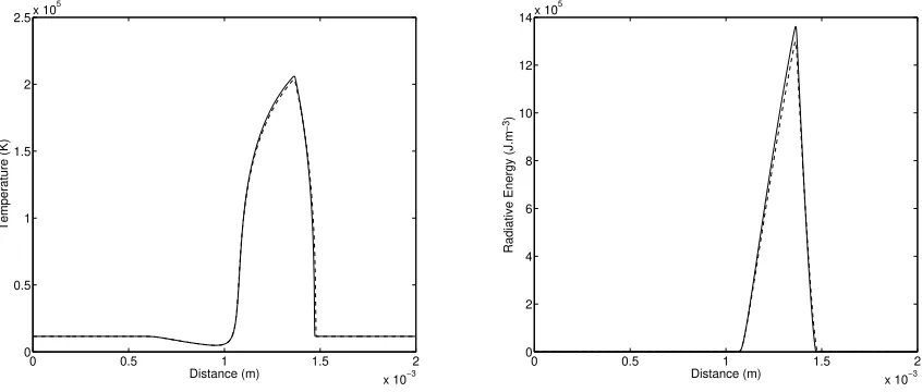
Figure 3. Results for M1 model (solid line) and diffusion model (dashed line) at timet= 40 ns.

Left: temperature profile versusx. Right: radiative energy profile versusx.

space step δx = δy = 10−6 m, where the piston initially fills 20 cells inx-space. Since we do not take into account ionization processes in our model, we roughly estimate it by dividing per 10 the mean molecular weight of krypton, which gives µ= 8.3798. Moreover, we assume that opacities are constant and equal to the space step. A comparison between results obtained with the M1 model and the diffusion approximation model at time t= 40 ns is shown on Figure 3. One can observe a very good quantitative and qualitative accordance between the two models, either for density and radiative energy. In this simulation, the maximal Mach number is found to be around 8. Let us notice that computational time is approximately 12 hours for a parallelized computation of 16 processors for the M1 model with HADES code and 28 minutes for a sequential computation using the diffusion approximation model. It has to be pointed out that using the M1 model, the CFL condition restricted significantly the time step in the hyperbolic part due to the speed of waves which depends on the speed of light. Consequently, it is worth dealing with the diffusion approximation model for optically thick flows rather than the full radiative transfer model for which computation times are much greater.

4.3.

Subcritical and supercritical shocks

This benchmark has been introduced by [5] and was used to validate several numerical codes for radiation hydrodynamic models (see [1], [2], [6], [7]). Depending on temperatures T− and T+ respectively observed at left-hand side and right-hand side of the shock, two cases occur: if the fluid velocity is sufficiently low, then T+T− and the shock is said to besubcritical, whereas for large enough fluid velocity, thenT−∼T+and the shock is said to besupercritical. In both cases, a temperature overshoot is found at the shock location. We have here simulated a cold medium with γ = 1.4 and µ= 1 in the initial configuration ρ1 = 7.78×10−7 kg m−3,

been taken constant and equal toκ= 3.1×10−8 m−1. Our computations have been performed on the spatial domain 7×108_{m discretized with 300 cells with a CFL number equal to 0.1. We impose a reflexive boundary} condition for the velocity at the left-hand side of the computational domain. Snapshots of the solutions are

0 1 2 3 4 5

x 108

0 200 400 600 800 1000 1200

Distance (m)

Temperature (K)

0 2 4 6 8 10

x 108

0 1000 2000 3000 4000 5000 6000

Distance (m)

Temperature (K)

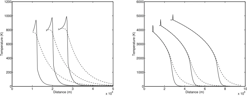
Figure 4. Snapshots of temperature profiles. Left: subcritical shock (u1=−6×103 m s−1)

at times (from left to right) 1.7×104 _{s, 2.8×10}4 _{s and 3.8×10}4_{s. Right: supercritical shock} (u1=−2×104m s−1) at times (from left to right) 4.0×103s, 7.5×103s and 1.3×104s (solid line: gas temperatureT; dashed line: radiative temperatureTR= (ER/aR)

1 4).

presented in Figure 4 at different times. Curves are plotted in the moving frame (that is with respect tox−u1t) in order to make a comparison with the ones obtained in the literature. The total CPU time was 9.4 s for the first simulation and 8.7 s for the second one. In both cases, our results are in good agreement with the ones obtained in the cited papers. For the subcritical shock, the increasing ofT− produces a flux of orderσRT24 that preheats the material ahead the front shock and locally generates a temperature overshoot. For the supercritical case, the overshoot temperature is also observed at the interface between pre-shock and post-shock states with similar temperatures.

4.4.

Radial test

We also performed a radial simulation on the cartesian domain [−8,8]×[−8,8] in a medium characterized by γ = 5/3, µ= 1 and that is assumed to be initially at rest with uniform density ρ0 = 10−8 kg m−3. We impose the Gaussian radiative energyER(x, y) = exp(−(x2+y2)) and assuming that the gas is in equilibrium

with radiation imply that initiallyE=ρkB(ER/aR)1/4/(γ−1). The numerical value of the densityρ0has been chosen in such a way thatE∼ER. We run the simulation with two sets of opacitiesκP =κR= 103m−1 and κP =κR= 105 m−1, for a 400×400 spatial discretization. The CFL number has been taken equal to 0.9 and

the simulation has been performed until timet= 10−3 s.

−80 −6 −4 −2 0 2 4 6 8 0.5

1 1.5 2 2.5 3 3.5x 10

−8

Distance (m)

Density (kg/m

3)

−8 −6 −4 −2 0 2 4 6 8

−3000 −2000 −1000 0 1000 2000 3000

Distance (m)

X velocity (m/s)

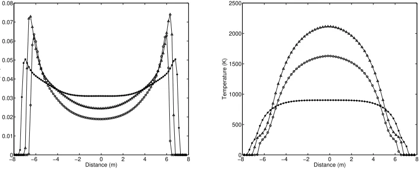
Figure 5. Trace ony= 0 for the density (left hand-side) and x-velocity (right hand-side) for

differentκP =κR=κ: κ= 105m−1(triangle),κ= 103m−1(asterisk) and pure hydrodynamic

case (disk).

−80 −6 −4 −2 0 2 4 6 8

0.01 0.02 0.03 0.04 0.05 0.06 0.07 0.08

Distance (m)

Ptot (Pa)

−80 −6 −4 −2 0 2 4 6 8

500 1000 1500 2000 2500

Distance (m)

Temperature (K)

Figure 6. Trace on y = 0 for different κP = κR = κ: κ = 105 m−1(triangle), κ = 103

m−1(asterisk) and pure hydrodynamic case (disk). Left: total pressure. Right: temperature.

4.5.

Quadrant test

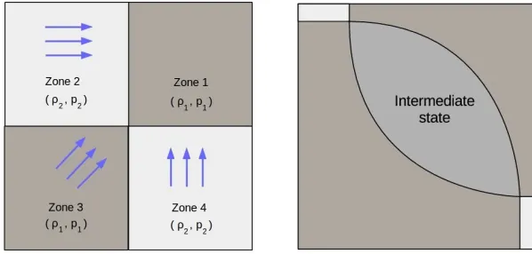
We finally perform a two-dimensional computation inspired by [10] where the initial data consists in constant states (see Figure 7) on the domain [0,1]×[0,1] separated into 4 different zones

(ρ, u, v, p)(x, y,0) = 

   

   

(ρ1, u1, v1, p1) = (1.1×10−7,0,0,11) ifx >0.5 andy >0.5

(ρ2, u2, v2, p2) = (5.065×10−8,8.939×103,0,3.5) ifx <0.5 andy >0.5 (ρ3, u3, v3, p3) = (1.1×10−7,8.939×103,8.939×103,11) ifx <0.5 andy <0.5

(ρ4, u4, v4, p4) = (5.065×10−8,0,8.939×103,3.5) ifx >0.5 andy <0.5

.

We deal with an overdensity and overpressure between zones 1, 3 and zones 2, 4 with symmetric velocity field (an horizontal and a vertical one for zones 2 and 4 and a diagonal one for the zone 3). The radiative energy is initialized to ER =aRT4 for a gas characterized by γ = 1.4 and µ = 1. One can refer to Figure 7 (left)

for a better understanding of the initial profile. Using this set of initial values, the resolution of the pure hydrodynamic problem exhibits shock waves between the different states with a nonconstant one that develops inside an increasing central domain (see Figure 7, right). Note that the interfaces between zones (1,2), (2,3), (3,4) and (4,1) are propagating with speeds given by Rankine-Hugoniot one-dimensional values. The solution is computed using 400 ×400 gridcells and the CFL number has been taken equal to 0.9.

Figure 7. Left: initial data. Right: structure of the solution of the Riemann problem involving

an intermediate state.

In Figure 8 are viewed the plots obtained for the density, first in a purely hydrodynamic configuration (left) and compared with the results in the diffusion regime (right), considered with the same initial states. In both cases, it can be observed the formation of the central structure delimited with circular shock waves. It means that even in the diffusion case, the general structure of the solution mimics the one in the absence of radiation. However, the density found in the diffusion case involves waves that once again propagate faster than in the hydrodynamic case. Moreover, the solution exhibits two dense regions in the poles of the structure in presence of radiation. This accumulation is also present when viewing the profile of radiative energy (see Figure 9, left). A slight density overshoot and a depletion effect at the center of the intermediate zone can be noticed. The plot of the trace of the density in the diagonal line that is presented in Figure 9 (right) for different values of opacities clearly confirms this effect. Qualitatively, this appears to be the same effect as the one observed in one-dimensional simulations: once again, the radiation magnifies both the values and the speed of propagation of density fronts. Let us finally mention that the cartesian crossed-line structure that is observed around the intermediate state in Figure 8 (right) is not a consequence of the directional splitting used in the method: the same simulation performed with aπ/4-angle rotation has given the same result. Indeed, these secondary waves are generated by the radiation processes.

5.

Discussion and perspectives

Figure 8. (x, y)-map of the density profile (×10−7 kg m−3) at timet = 10−6 s. Left: pure hydrodynamic case. Right: diffusion case (κP =κR= 0.1 m−1).

0 2 4 6 8 10 12 14

x 107 0.9

1 1.1 1.2 1.3 1.4 1.5 1.6

x 10−7

Distance (m)

Density (kg/m

3)

Figure 9. Left: (x, y)-map of the radiative energy profile (J m−3) at timet= 10−6 s. Right:

trace on the first diagonal axis for different κP =κR =κ: κ= 10−1 m−1(cross), κ = 10−2

m−1(triangle),κ= 10−3 m−1(diamond) and pure hydrodynamic case (disk).

whether on the acceleration of wave velocities or in the hydrodynamic quantities. In a forthcoming study, this model will be simulated in more realistic astrophysical configurations where numerical results could be compared with experimental data.

References

[1] F. Blach`ere,High-order asymptotic-preserving numerical scheme for radiation hydrodynamics, th`ese, Universit´e Nantes ;

Universit´e Bretagne Loire, 2016.

[2] B. Commerc¸on, R. Teyssier, E. Audit, P. Hennebelle, and G. Chabrier,Radiation hydrodynamics with adaptive mesh

[3] W. Dai and P. R. Woodward,Numerical simulations for radiation hydrodynamics. i. diffusion limit, Journal of

Computa-tional Physics, 142 (1998), pp. 182–207.

[4] B. Dubroca and J. Feugeas, Etude th´eorique et num´erique d’une hi´erarchie de mod`eles aux moments pour le transfert

radiatif, Academie des Sciences Paris Comptes Rendus Serie Sciences Mathematiques, 329 (1999), pp. 915–920.

[5] L. Ensman,Test problems for radiation and radiation-hydrodynamics codes, The Astrophysical Journal, 424 (1994), pp. 275–

291.

[6] M. Gonz´alez, E. Audit, and P. Huynh,HERACLES: a three-dimensional radiation hydrodynamics code, Astron. Astrophys.,

464 (2007), pp. 429–435.

[7] J. C. Hayes and M. L. Norman,Beyond Flux-limited Diffusion: Parallel Algorithms for Multidimensional Radiation

Hydro-dynamics, The Astrophysical Journals, 147 (2003), pp. 197–220.

[8] P. H. Hugoniot,M´emoire sur la propagation des mouvements dans les corps et sp´ecialement dans les gaz parfaits (deuxi`eme

partie), vol. 58, Journal de l’ ´Ecole Polytechnique, 1889.

[9] M. R. Krumholz, R. I. Klein, C. F. McKee, and J. Bolstad, Equations and algorithms for mixed-frame flux-limited

diffusion radiation hydrodynamics, The Astrophysical Journal, 667 (2007), p. 626.

[10] A. Kurganov and E. Tadmor,Solution of two-dimensional riemann problems for gas dynamics without riemann problem

solvers, Numerical Methods for Partial Differential Equations, 18 (2002), pp. 548–608.

[11] C. D. Levermore,Relating eddington factors to flux limiters, Journal of Quantitative Spectroscopy and Radiative Transfer,

31 (1984), pp. 149–160.

[12] R. B. Lowrie, D. Mihalas, and J. E. Morel,Comoving-frame radiation transport for nonrelativistic fluid velocities, Journal

of Quantitative Spectroscopy and Radiative Transfer, 69 (2001), pp. 291–304.

[13] C. Michaut, L. Di Menza, H. C. Nguyen, S. E. Bouquet, and M. Mancini,HADES code for numerical simulations of

high-mach number astrophysical radiative flows, High Energy Density Physics, 22 (2017), pp. 77–89.

[14] D. Mihalas,On laboratory-frame radiation hydrodynamics, Journal of Quantitative Spectroscopy and Radiative Transfer, 71

(2001), pp. 61–97.

[15] D. Mihalas and R. I. Klein,On the solution of the time-dependent inertial-frame equation of radiative transfer in moving

media to o(v/c), Journal of Computational Physics, 46 (1982), pp. 97–137.

[16] D. Mihalas and B. W. Mihalas,Foundations of radiation hydrodynamics, 1984.

[17] G. N. Minerbo,Maximum entropy eddington factors, Journal of Quantitative Spectroscopy and Radiative Transfer, 20 (1978),

pp. 541 – 545.

[18] G. C. Pomraning,The Equations of Radiation Hydrodynamics, Pergamon, NY, 1973.

[19] W. J. M. Rankine,On the thermodynamic theory of waves of finite longitudinal disturbance, Philosophical Transactions of

the Royal Society of London, 160 (1870), pp. 277–288.

[20] G. Strang,On the construction and comparison of difference schemes, SIAM J. Numer. Anal., 5 (1968), pp. 506–517.

[21] E. F. Toro,Riemann Solvers and Numerical Methods for Fluid Dynamics: A Practical Introduction., Springer - Verlag, 2nd

edition ed., 2006.

[22] E. F. Toro, M. Spruce, and W. Speares,Restoration of the contact surface in the hll-riemann solver, Shock Waves, 4

(1994), pp. 25–34.

[23] N. J. Turner and J. M. Stone,A Module for Radiation Hydrodynamic Calculations with ZEUS-2D Using Flux-limited

Diffusion, The Astrophysical Journal Supplement Series, 135 (2001), pp. 95–107.

[24] B. van Leer,On the relation between the upwind-differencing schemes of godunov, engquist-osher and roe, SIAM Journal on

Scientific and Statistical Computing, 5 (1984), pp. 1 – 20.

[25] Y. B. Zel’dovich and Y. P. Raizer,Physics of shock waves and high-temperature hydrodynamic phenomena, 1967.

[26] W. Zhang, L. Howell, A. Almgren, A. Burrows, and J. Bell,Castro: A new compressible astrophysical solver. ii. gray