1.
Introduction
The natural convective flow induced by thermal and solutal buoyancy forces that act on bodies with different geometries in a fluid-saturated porous medium is prevalent in many natural phenomena and has wide-ranging industrial applications. In atmospheric flows, for example, maintaining the purity of air or water is impossible because foreign mass may be present either naturally or in mixed form with air or water due to industrial emissions. Natural processes such as the attenuation of toxic waste in water bodies, the vaporization of mist and fog, photosynthesis, the drying of porous solids, transpiration, sea wind formation (wherein upward
convection is modified by Coriolis forces), and ocean current formation occur because of the thermal and solutal buoyancy forces that develop as a result of temperature difference, temperature concentration, or a combination of these two. Such forces are also encountered in several practical systems for industry-based applications, including heat exchanger devices, molten metals (for cooling), insulation systems, petroleum reservoirs, filtration systems, chemical catalytic reactors and processes, nuclear waste repositories, desert coolers, wet bulb thermometers, and frost formation in vertical channels.
Considering the importance of the above-mentioned fluid flow problems, extensive research has been carried out on these issues. Raju et al. [1], for instance, derived analytical and numerical
Analytical and numerical investigation of heat and mass transfer effects on
magnetohydrodynamic natural convective flow past a vertical porous plate
Rallabandi Srinivasa Raju
a*, Gampa Anitha
aand Gurejala Jithender Reddy
b aDepartment of Engineering Mathematics, GITAM University, Hyderabad, 502329, Medak (Dt), Telangana State, IndiabDepartment of Mathematics, VNR Vignana Jyothi Institute of Engineering and Technology, Hyderabad, Ranga Reddy (Dt), 500090, Telangana State, India.
Journal of Heat and Mass Transfer Research
Journal homepage: http://jhmtr.journals.semnan.ac.ir
A B S T R A C T
This study investigated the effects of the Hall current on the unsteady natural convective flow of a viscous, incompressible, and electrically conducting optically thick radiating fluid past a vertical porous plate in the presence of a uniform transverse magnetic field. Rosseland diffusion approximation was used to describe the radiative heat flux in the energy equation. Analytical and numerical solutions of coupled governing partial differential equations for fluid velocity, fluid temperature, and fluid concentration profiles were obtained via perturbation and finite element techniques, respectively. Graphs were used as bases for examining the effects of various dimensionless engineering parameters, namely, the Grashof number for heat and mass transfer, a magnetic field parameter, the Prandtl and Schmidt numbers, a thermal radiation parameter, the Hall parameter entering into the problem of primary and secondary velocities, and temperature and concentration profiles throughout the boundary layer. Expressions for skin friction, the Nusselt number, and the Sherwood number were derived and represented in tabular form. Results revealed that flow field and temperature distribution are considerably influenced by the thermal radiation parameter. The research also obtained limiting cases, which were found to be in good agreement with previously published results.
© 2017 Published by Semnan University Press. All rights reserved. DOI: 10.22075/jhmtr.2017.1503.1100
PAPER INFO
History:
Submitted 2017-01-07 Revised 2017-07-25 Accepted 2017-03-03
Keywords:
Heat and Mass transfer; Natural convection; Hall current; Porous medium;
Finite element method; Perturbation technique
Corresponding Author : Department of Engineering Mathematics, GITAM University, Hyderabad, 502329, Medak (Dt), Telangana State, India
solutions of unsteady magnetohydrodynamic (MHD) free convective flow over an exponentially moving vertical plate with heat absorption. Reddy and Raju [2] studied transient MHD free convective flow past an infinite vertical plate embedded in a porous medium with viscous dissipation. Raju et al. [3] probed into the application of the finite element method in the examination of unsteady MHD free convective flow past a vertically inclined porous plate. The authors included thermal diffusion and diffusion thermo effects in their analysis. Similarly, Raju et al. [4] used the finite element method to illuminate thermal diffusion and diffusion thermo effects on unsteady heat and mass transfer MHD natural convective Couette flow. Murthy et al. [5] studied heat and mass transfer effects on MHD natural convective flow past an infinite vertical porous plate in the presence of thermal radiation and the Hall current. Sivaiah and Raju [6] investigated finite element solutions of heat and mass transfer flow on the basis of the Hall current, heat sources, and viscous dissipation. Rao et al. [7] also examined finite element solutions of heat and mass transfer, this time with particular concentration on the MHD flow of a viscous fluid past a vertical plate under oscillatory suction velocity. Rao et al. [8] discussed chemical reaction effects on unsteady MHD free convective fluid flow past a semi-infinite vertical plate embedded in a porous medium with heat absorption. The combined influence of thermal diffusion and diffusion thermo on chemical reacted magnetohydrodynamic free convection from an impulsively started infinite vertical plate embedded in a porous medium studied by Jithender Reddy et al. [9] using finite element method. Ramya et al. [10] discussed the influence of chemical reaction on the MHD boundary layer flow of nanofluids over a nonlinearly stretching sheet with thermal radiation. Ramya et al. [11] studied the slip effect of the MHD boundary layer flow of nanofluid particles over a non-linearly isothermal stretching sheet in the presence of heat generation/absorption. Appling the finite element method, Rao et al. [12] obtained numerical solutions to MHD transient flow past an impulsively started infinite horizontal porous plate in a rotating fluid with the Hall current. Radiation and mass transfer flow past a semi-infinite moving vertical plate with viscous dissipation was examined via finite element analysis by Rao et al. [13]. The combined influence of thermal diffusion and diffusion thermo effects on unsteady hydromagnetic free convective fluid flow past an infinite vertical porous plate in the presence of chemical reaction was investigated by Raju et al. [14]. The effects of thermal radiation and heat source on unsteady MHD free convective flow past an infinite vertical plate with thermal diffusion and diffusion thermo effects were studied by Raju et al. [15]. The effects of a magnetic field on the flow field, heat transfer, and entropy generation of Cu–water nanofluid mixed
convection in a trapezoidal enclosure were investigated by Aghaei et al. [16]. Aghaei et al. [17] studied the effects of a magnetic field on the flow field and heat transfer of nanofluid with variable properties in a square enclosure with two heat sources.
The study of many transport processes existing in nature and in industrial applications, wherein heat and mass transfer is a consequence of buoyancy effects caused by the diffusion of heat and chemical species, is useful for improving a number of chemical technologies, such as polymer production, enhanced oil recovery, underground energy transport, ceramic manufacturing, and food processing. Heat and mass transfer from different geometries embedded in porous media finds numerous engineering and geophysical applications. For example, it is considered in the drying of porous solids, the use of thermal insulation, and the cooling of nuclear reactors. At high operating temperatures, radiation effects can be significant. Because many engineering processes are implemented at high temperatures, knowledge of radiation heat transfer is critical in the design of reliable equipment, nuclear plants, gas turbines, and various propulsion devices or aircraft, missiles, satellites, and space vehicles. The combination of heat and mass transfer problems with chemical reaction is equally important in many processes and has therefore received considerable attention in recent years. Such combination has found numerous applications in, for example, the design of chemical processing equipment, investigations of crop damage due to freezing, and the use of food processing and cooling towers. In this regard, Deka et al. [18] investigated the effects of first-order homogeneous chemical reaction on unsteady flow past an infinite vertical plate with constant heat and mass transfer. Muthucumaraswamy and Ganesan [19] discussed the effects of chemical reaction and injection on the flow characteristics of the unsteady upward motion of an isothermal plate. The MHD flow of a uniformly stretched vertical permeable surface in the presence of heat generation/absorption and chemical reaction was considered by Chamkha [20]. Ibrahim et al. [21] obtained an analytical solution for unsteady MHD free convective flow past a semi-infinite vertical permeable moving plate with a heat source and chemical reaction. Rahman et al. [22] studied heat transfer in micropolar fluid with temperature-dependent fluid properties along a non-stretching sheet.
in exploring radiation was addressed by other scholars. Cogley et al. [23], for example, showed that in an optically thin limit for a non-gray gas near equilibrium, the fluid does not absorb its own emitted radiation but absorbs the radiation emitted by boundaries. Satter and Hamid [24] investigated unsteady free convective interaction with thermal radiation in boundary layer flow past a vertical porous plate. Vajravelu [25] shed light on the flow of a steady viscous fluid and heat transfer characteristics in a porous medium by considering different heating processes. Hossain and Takhar [26] considered radiation effects on the mixed convective boundary layer flow of an optically dense viscous incompressible fluid along a vertical plate with uniform surface temperature. Raptis [27] investigated the steady flow of a viscous fluid through a porous medium bounded by a porous plate subjected to a constant suction velocity through the presence of thermal radiation. Makinde [28] examined transient free convective interaction with the thermal radiation of an absorbing emitting fluid along a moving vertical permeable plate. The effects of chemical reaction and radiation absorption on unsteady MHD free convective flow past a semi-infinite vertical permeable moving plate with a heat source and suction was studied by Ibrahim et al. [29]. Bakr [30] presented an analysis of MHD free convection and mass transfer adjacent to a moving vertical plate for micropolar fluid in a rotating frame of reference under the presence of heat generation/ absorption and a chemical reaction.
When the density of an electrically conducting fluid is low and/or when an applied magnetic field is strong, the Hall current is produced in the flow field. The Hall current plays an important role in determining the features of flow problems because it induces econdary flow in the flow field. With this consideration in mind, several researchers comprehensively investigated hydromagnetic free convective flow past a flat plate with Hall effects under different thermal conditions. Some of these works are those conducted by Pop and Watanabe [31], Abo-Eldahab and Elbarbary [32], Takhar et al. [33], and Saha et al. [34]. Note that the Hall current‘s inducement of secondary flow in the flow field resembles the characteristics of Coriolis force. Comparing the individual effects of these two phenomena and their combined influence on fluid flow problems is therefore a crucial component of fluid flow research. Such effort has been initiated by certain studies, such as that of Narayana et al. [35], who probed into the effects of the Hall current and radiation–absorption on the MHD natural convective heat and mass transfer flow of a micropolar fluid in a rotating frame of reference. Seth et al. [36] investigated the effects of the Hall current and rotation on the unsteady hydromagnetic natural convective flow of a viscous, incompressible, electrically conducting, and heat-absorbing fluid past
an impulsively moving vertical plate with ramped temperature in a porous medium. The authors also took the effects of thermal diffusion into account.
The main purpose of the present investigation was to illuminate the effects of the Hall current and thermal radiation on unsteady MHD natural convective heat and mass transfer flow past a vertical porous plate. We assumed that the plate is embedded in a uniform porous medium and oscillates in time with a constant frequency in the presence of a transverse magnetic field. Governing equations were solved numerically using the finite element technique, and numerical results were derived for various values of the physical parameters of interest.
2.
Mathematical formulations
The fundamental equations that govern the motion of an incompressible, viscous, and electrically conducting fluid in the presence of a magnetic field are as follows [37]:
Equation of continuity:
0
v
(1)Momentum equation:
v
k
v
g
B
J
P
v
v
t
v
2
(2)
Energy equation:
y q T T
v t T
C r
p
2
(3)
Species continuity equation:
v
C
D
C
t
C
2 (4)Kirchhoff’s first law:
0
J
(5)General Ohm’s law, with consideration for Hall effects:
e
e e
e
p e B v E B J B J
10
(6)
Gauss’s law of magnetism:
0
Fig. 1. Geometry of the problem
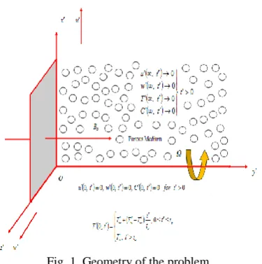
The unsteady flow of an electrically conducting fluid past an infinite vertical porous flat plate that coincides with the
x
- axisy
0
was considered. For this case, thermal diffusion, the Hall current, and heat sources in the presence of a uniform transverse magnetic field were also taken into account. Our investigation was underlain by the following assumptions:i. The coordinate system is chosen in such a way that the
x
- axis runs along the plate in an upward direction, and the y′-axis runs normal to the plane of the plate immersed in the fluid. ii.A uniform transverse magnetic fieldB
o isapplied in a direction parallel to the
y
- axis. iii.Initially (i.e., at timet
0
), both the fluid andplate are at rest and have uniform temperature
T
. Species concentration on the surface of the plate and at every point within the fluid is maintained at uniform concentrationC
.iv.The temperature at the surface of the plate is increased to uniform temperature
T
w
, and species concentration on such surface is raised to uniform species concentrationC
w
and maintained at this level thereafter.v. Given that the plate is of infinite extent in the
x
direction and is electrically non-conducting, all physical quantities, except pressure, depend only on
y
andt
.vi.No applied or polarized voltages exist, thereby rendering the effects of fluid polarization negligible. This corresponds to a case wherein no energy is incorporated into or extracted from fluid by electrical means [38].
vii.The magnetic field induced by fluid motion is negligible in comparison to the applied magnetic field. This assumption is justified because the magnetic Reynolds number is very small for the
liquid metals and partially ionized fluids that are commonly used in industrial applications [38]. viii.No voltage is applied, suggesting the absence of
an electric field.
ix.All the fluid properties, except density in the buoyancy force terms, are constant.
We introduce a coordinate system
x
,
y
,
z
, in which thex
- axis is positioned vertically upwards, they
- axis is normal to the plate directed into the fluid region, and thez
- axis runs along the width of the plate. Letk
w
j
v
i
u
v
ˆ
ˆ
ˆ
be the velocity,k
J
j
J
i
J
J
xˆ
yˆ
zˆ
be the current density at pointp
x
,
y
,
z
,
t
, andB
B
0J
ˆ
be the applied magnetic field, withi
ˆ
,
ˆ
j
,
k
ˆ
being the unit vectors along thex
- axis,y
- axis, andz
- axis, respectively. Because the plate is of infinite length in thex
andz
directions, all values, except perhaps that of pressure, are independent ofx
andz
. Eq. (1) yields0
y
v
(8)which is trivially satisfied by
0
V
v
(9) whereV
0 is a constant, andV
0
0
. Therefore, velocity vectorv
is obtained usingk
w
j
V
i
u
v
ˆ
0ˆ
ˆ
(10)Eq. (7) is satisfied by
j
B
B
0ˆ
(11)Eq. (5) is reduced to
0
y
J
y(12)
which shows that
J
y
constant. Given that the plate is non-conducting,J
y
0
at the plate and, hence,0
yJ
at all points in the fluid. Accordingly, the current density is given byk
J
i
J
Under assumptions (iv) and (v), Eq. (6) takes the form
J
B
v
B
B
m
J
0
(14)
where
m
e
e is the Hall parameter. Eqs. (10), (11), (13), and (14) yield
u mw
m B J and w u m m B J z x 2 0 2 0 1 1
(15)With the above assumptions the usual boundary layer, and Boussinesq‘s approximation, Eqs. (2) to (4) are reduce to the following forms:
C
C
g
T
T
g
u
k
w
m
B
m
u
B
m
y
u
y
u
v
t
u
2 2 0 2 0 2 2 21
1
1
(16)
k w m w u m B y w y w v t w
02 22 2
1 (17)
y q C y T T C y T T v t T T r p p
1 2 2 (18)
2 2y
C
C
D
y
C
C
v
t
C
C
(19)For an optically thick fluid, both emission and self-absorption exist, and the absorption coefficient is usually wavelength dependent and large. These features enable the use of Rosseland approximation for the radiative heat flux vector. Thermal radiation is assumed present in the form of a unidirectional flux in the
y
direction, that is,q
r (transverse to the vertical surface). Using the Rosseland approximation [39], radiative heat fluxq
r is derived thus:y
T
k
q
e sr
43
4
(20)where
sis the Stefan–Boltzmann constant, andk
edenotes the mean absorption coefficient. Note that the adoption of Rosseland approximation limited the
present analysis to optically thick fluids. If temperature differences within flow are sufficiently small, then Eq. (20) can be linearized by expanding
4
T
in the Taylor series aboutT
, which, after disregarding higher-order terms, takes the following form:
3 3 44 4
3
4
4
T
T
T
T
T
T
T
T
(21)Using Eqs. (21) and (20) in the last term of Eq. (18) derives 2 2 3
3
16
y
T
k
T
y
q
e h s r
(22)Introducing Eq. (22) into Eq. (18) produces the energy equation in the following form:
2 2 3 2 23
16
y
T
C
k
T
y
T
C
y
T
T
v
t
T
T
p e s p
(23)In Eq. (18), viscous dissipation and Ohmic dissipation are disregarded, and in Eq. (19), the term arising from chemical reaction is absent. We now use
y
t
T
y
t
T
V
v
0,
,
,
and
y
t
C
y
t
C
,
,
subject to boundary conditions
0
:
,
,
0
,
0
:
0
y
at
t
t
T
T
T
T
t
t
y
all
for
C
C
T
T
w
u
t
o w o
y
as
C
C
T
T
w
u
y
at
C
C
t
t
T
T
T
T
w
u
t
w o w,
,
0
,
0
0
,
,
0
,
0
:
0
as
y
T
T
y
at
T
T
t
t
o:
w0
(24)0
V
t
o
. Let us introduce the followingdimensionless quantities: a k T F k V K D Sc C V B M V b g Gc V a g Gr b C V w w V u u t V t y V e s p
, 4 , 4 , , Pr , 4 , 4 , 4 , , , , 4 , 3 2 2 0 3 0 2 0 3 0 3 0 0 0 ' 2 0 0 (25)Eqs. (16) to (19) are converted into the following non-dimensional forms, respectively:
K
u
Gc
Gr
mw
u
m
M
u
u
t
u
2 22
1
4
4
(26)
K
w
w
mu
m
M
w
w
t
w
2 2 21
4
4
(27)2 2
3
4
1
Pr
4
4
F
t
(28) 2 2 4 4
Sc t (29)The corresponding boundary condition (23) in non-dimensional form is
as at t at t t as w u at t w u t all for w u t 0 , 0 0 1 : 1 0 : 1 0 , 0 , 0 , 0 0 1 , , 0 , 0 : 0 0 , 0 , 0 , 0 : 0 (30)
For practical engineering applications and the design of chemical engineering systems, the values of interest include the skin friction coefficient, the couple stress coefficient, the Nusselt number, and the Sherwood number. The local skin friction coefficient, which signifies surface shear stress, is defined as
0 2
0
2, (0)
u u V y u u C o y w w wf (31)
The couple stress coefficient on a wall is given by
0 2
0
2
,
(
0
)
w
w
V
y
w
w
w
C
o y w w ww (32)
The local Nusselt number embodies the ratio of convective to conductive heat transfer across (normal to) a boundary and is a quantification of surface temperature gradient (heat transfer rate on a wall). It is defined as
0
)
(
)
(
y w uy
T
T
T
x
x
N
then 0 ) ( x e u R x N Nu (33)Finally, the local Sherwood number, which encapsulates the ratio of convective to diffusive mass transport and simulates the surface mass transfer rate, is defined thus
0
)
(
)
(
y w hy
C
C
C
x
x
S
then 0)
(
x e hR
x
S
Sh
(34)where
x
V
R
o ex
.3.
Solution Method
3.1. Numerical solution via the finite element method
The finite element method was implemented to obtain numerical solutions (25) to (28) under boundary condition (29). This technique is extremely efficient and generates robust solutions to complex coupled, nonlinear, multiple-degree differential equation systems. The fundamental steps of the method are summarized below. An excellent description of finite element formulations was also provided by Bathe [40] and Reddy [41].
3.1.1 Step 1: Discretization of a domain into elements
An entire domain is divided into a finite number of sub-domains—a process known as the discretization of the domain. Each sub-domain is termed a ―finite element,‖ and a collection of elements is designated as the ―finite element mesh.‖
3.1.2. Step 2: Derivation of the elements
algebraic expressions among the unknown parameters of finite element approximation) involves the following steps:
a. Construct the variational formulation of the differential equation.
b. Assume the form of the approximate solution over a typical finite element.
c. Derive the finite element by substituting the approximate solution into the variational formulation.
These steps result in a matrix equation of the form
e
e eF
u
K
, which defines the finite elementmodel of the original equation.
3.1.3. Step 3: Assembly of elements
The algebraic so obtained is assembled by imposing ―inter-element‖ continuity conditions. This assembly yields a large number of algebraic that constitute a global finite element model, which governs the entire flow in the domain.
3.1.4. Step 4: Imposition of boundary conditions
The physical boundary conditions defined in (29) are imposed on the assembled algebraic.
3.1.5. Step 5: Solution of assembled elements
The final matrix equation can be solved through a direct or indirect (iterative) method. For computational purposes, coordinate
is varied from 0 to
max
10
, where
max represents infinity (i.e., external to the momentum, energy, and concentration boundary layers). The entire domain is divided into a set of 100 line segments of equal width (0.1), with each element being two-noded.3.1.6. Step 6: Variational formulation
The variational formulation associated with (25) to (28) over a typical two-noded linear element
e,
e1
is given by
0
4
4
1 1 2 2 1
d
Gc
Gr
Bmw
u
Z
u
u
t
u
w
e e (35)0
4
4
1 2 2 2 2
d
Bmu
w
Z
w
w
t
w
w
e e (36)0
3
4
1
Pr
4
4
1 2 23
d
F
t
w
e e (37)0
4
4
1 2 24
d
Sc
t
w
e e (38)where
,
1
m
2M
B
1 1,K B Z
K B
Z2 1 , and
,
1
w
w
2,
w
3,
andw
4 are arbitrary test functions that may be viewed as variations inu
,
w
,
, and
, respectively. After reducing the order of integration and nonlinearity, we arrive at the following system of equations:
0
4
4
1 1 1 1 1 1 1 1 1 1 1
e e e eu
w
d
w
Gc
w
Gr
w
Bmw
u
w
Z
u
w
u
w
t
u
w
(39)
04 4 1 1 2 2 2 2 2 2 2
e e e e w w d w Bmu w w Z w w w w t w w (40)
0
Pr
3
4
1
3
4
1
Pr
4
4
1 1 3 3 3 3
e e e ew
F
d
w
F
w
t
w
(41)
0
4
4
1 1 4 4 4 4
e e e eSc
w
d
w
Sc
w
t
w
(42)3.1.7. Step 7: Finite element formulation
,
2 1
j e j e ju
u
,
2 1
j e j e jw
w
,
2 1
j e j e j
,
2 1
j e j e j
(43)with
w
1
w
2
w
3
w
4
(
i
1
,
2
),
e i
where,
e ju
w
ej,
ej , and
ej are the primary velocity, secondary velocity, temperature, and concentration, respectively, at thejth
node of the typicaleth
element
e,
e1
. Here,
ie represents the shape functions of
e,
e1
and are taken ase e e e
1 11 and ,
1 2 e e e e
1
ee
(44)The finite element model of the
eth
element thus formed is given by
e e e ew
u
K
K
K
K
K
K
K
K
K
K
K
K
K
K
K
K
44 43 42 41 34 33 32 31 24 23 22 21 14 13 12 11 (45)
e e e ew
u
M
M
M
M
M
M
M
M
M
M
M
M
M
M
M
M
44 43 42 41 34 33 32 31 24 23 22 21 14 13 12 11
e e e eb
b
b
b
4 3 2 1where
K
mn,
M
mn
and
(
,
1
,
2
,
3
,
4
)
,
,
,
,
,
,
,
n
m
b
and
w
u
w
u
me e e e e e e e e
arethe set of matrices of orders
4
4
and4
1
, respectively, and the /' (dash) indicates
d
d . These
matrices are defined as follows:
, 4 4 1 1 1 1 11
d Z d d K e e e e e e e j e i e j e i e j e i ij
d
Bmw
K
e e e i ij
1 12 ,
d
Gc
Gr
K
e e e j e i ij
1 13 ,
,
111
d
M
e e e j e i ij
K
ij21
K
ij24
0
,
,
0
14 13 12
14
ij ij ij
ij
M
M
M
K
,
1
23
d
Bm
K
e e e j e i ij
,
0
24 2321
ij ij ij
M
M
M
M
ij31
M
ij32
M
ij34
0
,
,
122
d
M
e e e j e i ij
K
ij31
K
ij33
K
ij34
0
,
,
1
33
d
M
e e e j e i ij
K
ij41
K
ij42
K
ij43
0
,
,
3
4
1
Pr
4
4
1 1 32
d
F
d
K
e e e e e j e i e j e i ij
,
1 2
e ew
b
ie ie
M
ij31
M
ij32
M
ij34
0
,
,
4
4
1 1 1 2 22
d
Z
d
d
K
e e e e e e e j e i e j e i e j e i ij
,
144
d
M
e e e j e i ij
,
1 1
e eu
b
ie ie
,
3
4
1
Pr
1 3
e eF
b
e i e i
1 4
e eSc
b
e i e i
The entire domain is divided into a set of 100 intervals of equal length (0.1). At each node, two functions are to be evaluated. The assembly of the elements therefore produces a set of 123. Given that the system derived after the assembly are nonlinear, an iterative scheme is employed to solve the matrix system. Specifically, the Gauss elimination method is used, thereby maintaining an accuracy of 0.0005.
3.2. Analytical solution via perturbation technique
To find the solution of the system of partial differential equations (25) to (28) in the neighborhood of the plate under condition (29), we assume a perturbation of the forms
2
int 1
int 0
2
,
t
u
e
u
e
u
u
(46)
2
int 1
int 0
2
,
t
w
e
w
e
w
w
(47)
int 21 int 0
2
,
t
e
e
(48)
int 21 int 0
2
,
t
e
e
(49)From Eqs. (45) to (48), we derive
2
int 1 int
2
e
u
e
u
u
u
o
(50)
2
int 1 int 2
2
2
e
u
e
u
u
u
o
(51)
2
int 1
int
2
in
e
u
in
e
u
t
u
(52)
2
int 1 int
2
e
w
e
w
w
w
o
(53)
2
int 1 int 2
2
2
e
w
e
w
w
w
o
(54)
2
int 1
int
2
in
e
w
in
e
w
t
w
(55)
2
int 1 int
2
e
e
o (56)
2
int 1 int 2
2
2
e
e
o (57)
2
int 1
int
2
e
in
e
in
t
(58)
2
int 1 int
2
e
e
o (59)
2
int 1 int 2
2
2
e
e
o (60)
2
int 1
int
2
e
in
e
in
t
(61)Substituting Eqs. (45) to (60) into Eqs. (25) to (28), equating harmonic and non-harmonic terms, and disregarding the higher-order terms of
O
2yield the following set of equations:
0
4
4
u
o
u
o
Zu
o
Gr
o
Gc
o
Bmw
o
(52)0
4
4
w
o
w
o
Z
1w
o
Bmu
o
(63)0
Pr
4
o oo
F
(64)
0
4
oo
Sc
(65)0
4
4
u
1
u
1
Z
2u
1
Gr
1
Gc
1
Bmw
1
(66)0
4
4
w
1
w
1
Z
3w
1
Bmu
1
(67)0
Pr
4
1 1 11
X
(68)0
4
1 11
Sc
inSc
(69)0
4
4
u
2
u
2
Z
2u
2
Gr
2
Gc
2
Bmw
2
(70)0
4
4
w
2
w
2
Z
4w
2
Bmu
2
(71)0
Pr
4
2 2 22
X
(72)0
4
2 22
Sc
inSc
(73)where the prime denotes differentiation with respect
to
and,
1
2m
M
B
1
,
K
B
Z
,
1
1
K
B
Z
Z2 Z in,Z
3
Z
1
in
,
,
1
4
Z
in
Z
X
1
in
Pr
F
,
X
2
in
Pr
F
.The corresponding boundary conditions can be written as follows:
as
w
w
w
u
u
u
at
w
w
w
u
u
u
o o o o o o o o0
,
0
,
0
,
0
,
0
,
0
,
0
,
0
,
0
,
0
,
0
,
0
0
0
,
0
,
1
,
1
,
1
,
1
,
0
,
0
,
0
,
0
,
0
,
0
2 1 2 1 2 1 2 1 2 1 2 1 2 1 2 1 (74)Case 2: Ramped temperature
as
w
w
w
u
u
u
at
w
w
w
u
u
u
o o o o o o o o0
,
0
,
0
,
0
,
0
,
0
,
0
,
0
,
0
,
0
,
0
,
0
0
0
,
0
,
1
,
0
,
0
,
0
,
0
,
0
,
0
,
0
,
0
,
0
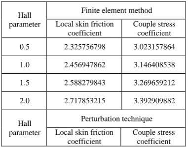
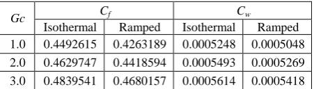
2 1 2 1 2 1 2 1 2 1 2 1 2 1 2 1 (75)Solving Eqs. (61) to (72) using boundary conditions (74) and (75) yields the expressions for primary and secondary velocities, temperature, and concentration. We obtained a comprehensive range of solutions to the converted conservation equations. To test the validity of the numerical finite element computations, we compared the local skin friction and couple stress coefficients and the Nusselt and Sherwood numbers in Tables 1 to 3 with the solutions obtained using the perturbation technique. The tables show that the results are in excellent agreement. As the numerical solutions are highly accurate, the values of
u
,
w
,
,
and
that correspond to the analytical and numerical solutions are very close to one another.Table 1:Comparison of local skin friction coefficient and couple stress coefficient with Gr = 6.0, Gc = 5.0, Pr = 0.71, F = 0.5, Sc = 0.6, and t = 0.5
Hall parameter
Finite element method Local skin friction
coefficient
Couple stress coefficient 0.5 2.325756798 3.023157864 1.0 2.456947862 3.146408538 1.5 2.588279843 3.269659212 2.0 2.717853215 3.392909882 Hall
parameter
Perturbation technique Local skin friction
coefficient
Couple stress coefficient
2.3257567990 3.02315786301 0.5 2.4569478630 3.14640853700 1.0 2.5882798440 3.2696592110 1.5 2.7178532160 3.39290988101 3.3. Accuracy of analytical and numerical solutions
Table 2: Comparison of local Nusselt number with Gr = 5.0, Gc = 5.0, Pr = 0.71, m = 0.5, Sc = 0.6, and t = 0.5
Radiation number Finite element method Perturbation technique 2.0 0.349673412 0.3496734130 1.5 0.407029841 0.4070298420 1.0 0.464386268 0.46438626900 0.5 0.521746697 0.5217466980
Table 3: Comparison of local Sherwood number with Gr = 6.0, Gc = 5.0, Pr = 0.71, F = 0.5, m = 0.5, and t = 0.5
Schmidt number Finite element method Perturbation technique 0.22 0.4348793152 0.4348793152 0.30 0.4237549217 0.4237549217 0.60 0.419679342 0.412679342 0.78 0.391582079 0.401582079
Table 4: Comparison of current local Sherwood number (Sh) values with the results of Sharma and Chaudhary [37]
Analytical results of Sharma and Chaudhary [37]
Sh
Sc = 0.22 Sc = 0.30 Sc = 0.78
0.2200 0.3000 0.7800 0.0800 0.1200 0.3800 - 0.1700 - 0.2100 - 0.4100 - 0.2700 - 0.3500 - 0.8100 - 0.0800 - 0.1200 0.3900 0.2100 0.2600 0.4400
Present numerical results
Sc = 0.22 Sc = 0.30 Sc = 0.78
0.218862 0.295247 0.774285 0.079562 0.119627 0.376248 - 0.169821 - 0.209634 - 0.409631 - 0.269824 - 0.349625 - 0.806431 - 0.079562 - 0.119627 0.382645 0.209634 0.259647 0.436921
4.
Code Validation
corresponds to the case computed by Sharma and Chaudhary [37] in the absence of thermal radiation and phase angle, with the authors adopting different Schmidt numbers and keeping other parameters constant. The results of the evaluation are presented in table 4. This favorable comparison lends confidence to the accuracy of the numerical procedure in the current work. The developed code can therefore be used with great confidence in the study of the problem considered in this paper.
5.
Results and Discussion
To analyze the effects of the Hall current, thermal buoyancy force, concentration buoyancy force, thermal diffusion, mass diffusion, thermal radiation, and time on the flow field, numerical values of the primary and secondary fluid velocities in the boundary layer region (computed from numerical solutions (38) and (39)) were plotted graphically against boundary layer coordinate η in Figs. 2 to 15 for various values of the Hall current parameter (m), the thermal Grashof number for heat transfer (Gr), the Grashof number for mass transfer (Gc), the Prandtl number (Pr), the Schmidt number (Sc), the thermal radiation parameter (F), and time (t). In the plotting, we set magnetic paramount permeability parameter K to0.5, Pr to0.71, and Sc to0.22.
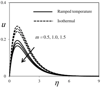
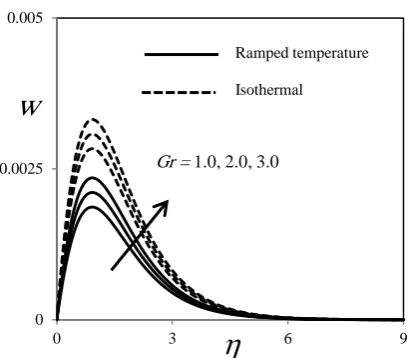
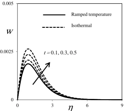
Figs. 2 to 15 indicate that for both ramped temperature and isothermal plates, primary velocity u
and secondary velocity w attain distinctive maximum values near the surface of the plate, after which the values decrease appropriately with increasing boundary layer coordinate η and thereby approach the free stream value. The primary and secondary fluid velocities are also slower in the ramped temperature plate than in the isothermal plate.
Fig. 2. Primary velocity profiles at Gr = 6, Gc = 5, Pr = 0.71, Sc = 0.6, F = 5, and t = 0.5.
Fig. 3. Secondary velocity profiles at Gr = 6, Gc = 5, Pr = 0.71, Sc = 0.6, F = 5, and t = 0.5.
Fig. 4. Primary velocity profiles at m = 0.5, Gc = 5, Pr = 0.71, Sc = 0.6, F = 5, and t = 0.5.
Fig. 2 illustrates that the primary velocity retards near the plate when Hall parameter m increases. Fig. 3 shows that the secondary velocity increases near the plate and decreases away from the plate with an increase in Hall parameter m. The momentum boundary layer thickness increases with increasing m. The Hall parameter exerts marked effects on the secondary velocity profiles because effective conductivity σ/(1+m2) decreases as m increases. For small values of m, the term 1/(1+m2) decreases, thereby increasing the resistive magnetic force and suppressing the fluid velocity components. This result is a new phenomenon, which emerges as a result of the inclusion of Hall currents. The case m = 0 corresponds to the disregard of Hall effects. Moreover, the primary and secondary profiles approach their classical hydrodynamic values when the Hall parameter tends to infinity. This finding is attributed to the fact that the magnetic force terms approach 0 for very large values of the Hall parameter.
0 0.2 0.4
0 3 6 9
u
η
m= 0.5, 1.0, 1.5Ramped temperature Isothermal
0 0.0025 0.005
0 3 6 9
w
η
m= 0.5, 1.0, 1.5Ramped temperature Isothermal
0 0.2 0.4
0 3 6 9
u
η
Gr= 1.0, 2.0, 3.0Fig. 5. Secondary velocity profiles at m = 0.5, Gc = 5, Pr = 0.71, Sc = 0.6, F = 5, and t = 0.5.
Fig. 6. Primary velocity profiles at m = 0.5, Gr = 6, Pr = 0.71, Sc = 0.6,