C. Besse, O. Goubet, T. Goudon & S. Nicaise, Editors
ANISOTROPY AND VORTICES IN BOSE EINSTEIN CONDENSATES
Amandine Aftalion
1Abstract. The fast rotation of a Bose Einstein condensate in a harmonic trap leads to a hexagonal lattice of vortices, called the Abrikosov lattice. Vortices are described as the zeros of the condensate wave function, which is a solution to a nonlinear Schrdinger equation type. We study the solutions of this equation on a specific eigenspace of the limiting problem, the Lowest Landau Level. Upper and lower bounds for the energy allow to determine the presence of a vortex lattice or the lack of visible vortices, as a function of the anisotropy and the rotation. The study of the critical regime is open and would need some numerical simulations. This constitutes a project in collaboration with Xavier Blanc and Nicolas Lerner.
1.
Introduction
Vortices in classical fluids are often related to turbulent phenomena, in hurricanes or typhoons for instance. In quantum fluids, such as Bose Einstein condensates (BEC), quantized vortices appear when the fluid is rotating and they provide an evidence of superfluidity. The aim of this paper is to make a review of mathematical issues related to vortices in fast rotating BEC. This is based on the papers [4, 6–8].
1.1.
Physical context
The phenomenon of condensation was predicted in 1925 by Einstein, on the basis of a paper by Bose: for a gas of non interacting particles, below a certain temperature, there is a phase transition where a macroscopic fraction of the gas gets condensed, that is, all the atoms occupy the state of lowest energy and are described by the same wave function, which is also the wave function of the condensate. There was no experimental evidence of this phenomenon, since at the densities and temperature required by the theory, all materials were in the solid state. The development of cooling techniques [10] led in 1995, to the achievement of Bose Einstein condensation in atomic gases by the Jila group in Boulder (Cornell, Wiemann [12]), and very soon afterwards by the MIT group (Ketterle [15]), which was awarded with the Nobel Prize for Physics in 2001. Now, many properties of these systems are studied both experimentally and theoretically. We refer to the books by Pethick-Smith [19] and Pitaevskii-Stringari [20] for more details on the physics. An important issue is the relationship between Bose Einstein condensation and superfluidity, in particular through the existence of vortices. A BEC is a quantum macroscopic object described by a macroscopic wave functionψ (complex-valued order parameter). For ψ = √ρeiS, vortices are lines of singularities along which ρ = 0 and around which (1/(2π))H
∇S·dr is an integer: ∇S is a superfluid velocity. There are two classical experiments which illustrate the quantum fluid behaviour and are addressed on a mathematical ground in a book by the author [2]. One consists in stirring a laser beam along the condensate in a translation movement: there is a critical velocity below which the movement is dissipationless and beyond which the stirring produces vortices, as in the moving of an object
1 CNRS, Universit´e Pierre et Marie Curie-Paris6, UMR 7598, Laboratoire Jacques-Louis Lions, 175 rue du Chevaleret, Paris
F-75013 France
c
EDP Sciences, SMAI 2009
in a superfluid. These aspects are described in [2], and will not be addressed here. In another experiment, achieved in the group of Jean Dalibard in Paris [17], a trapped system, which has a cigar shape, is rotated with a ”spoon”, like coffee in a cup. For small angular velocities, no modification of the condensate is observed. For sufficiently large angular velocities, the condensate behaves like a quantum fluid and, unlike coffee, vortices are detected in the system. When the rotational velocity is increased, the number of singularity lines increases and they get ordered through an Abrikosov lattice [1,9] (see Figure 1). The study of the lattice is at the core of very recent works [5, 11, 13, 14, 23] in the condensed matter physics community. We intend to address these aspects mathematically here.
1.2.
Mathematical setting
The study of interacting nonuniform quantum gases at zero temperature can be made in the framework of the Gross-Pitaevskii energy. The field operator used to describe quantum phenomena can be replaced by a classical field ψ, also called the order parameter or wave function of the condensate. We are interested in stationary phenomena: thus in the frame rotating at angular velocity Ω˜ = ˜Ωe3, the trapping potential and the wave function are time independent. In the experimental device, the rotation is obtained thanks to a laser beam imposed on the magnetic trap holding the atoms to create a harmonic anisotropic rotating potential. The wave functionψminimizes the following energy, called the Gross Pitaevskii energy, which includes in this order a kinetic contribution, a term due to rotation, a term due to the presence of a harmonic trapping and a term due to atomic interactions:
Z
R3
~2
2m|∇ψ|
2
−~Ω˜×x·(iψ,∇ψ) +m 2
3
X
i=j
ω2jx2j|ψ|2+N g3D|ψ|4, (1)
under the constraintR
|ψ|2= 1. Here,g
3D= 4π~2a0/m, wherea0is the scattering length describing interactions,
N is the number of atoms, m is the atomic mass,x= (x1, x2, x3), ωj is the trapping frequency along thejth direction, and (iψ,∇ψ) denotes the scalar product in Cso that it is equal to (iψ∇ψ¯−iψ¯∇ψ)/2.
We defineω=p(ω2
1+ω22)/2,d= (~/mω)1/2, the characteristic length of the harmonic oscillator. Rescaling distances byd, that is settingφ(x) =d3/2ψ(dx), and Ω = ˜Ω/ω
1, the energy becomes, in units of~ω,
E3D(φ) =
Z
R3
1 2|∇φ|
2
−Ω×x·(iφ,∇φ) +1 2((1−ν
2)x2
1+ (1 +ν2)x22+β2x32)|φ|2+ 4πN a0|φ|4 (2)
underR
|φ|2= 1. We have set 1−ν2=ω2
1/ω2andβ=ω3/ω. If Ω> √
1−ν2, the energy is not bounded below: the rotating force is stronger than the trapping potential. Our asymptotic regime of fast rotation will be when Ω reaches Ωc=√1−ν2.
There are two distinct regimes of rotation according to the value of Ω. For low rotational velocity, there is a transition from none to a few vortices in the system, and their characteristic size is much smaller than their inter distance. We refer to [2] for more details on this regime also known as the Thomas Fermi regime, which requires the introduction of a small parameter. The other regime is at high rotational velocity, that is when Ω is close to the critical trapping frequency Ωc=√1−ν2. Then, the centrifugal force nearly balances the trapping force, the condensate expands and the number of vortices diverges. There is a dense lattice for which vortices have approximately the same size as their inter distance.
1.3.
Main results
We setν = 0 in the energy (2) and write the first two terms as the expansion of a complete square, and thus subtract the extra term to find:
E3D(ψ) =
Z
IR3
1
2|∇ψ−iΩ×xψ| 2+1
2(1−Ω 2)
|r|2|ψ|2+1 2β
2x2
3|ψ|2+ 4πN a0|ψ|4, (3)
wherer= (x1, x2), under the constraintRIR3|ψ|2= 1. We assume thatψ∈ H3Ddefined by
H3D=ψ∈H1(IR3), s.t. E3D(ψ)<∞ . (4)
Our regime of interest is when Ω tends to 1. It displays a strong analogy with Quantum Hall physics: the first part of the Gross Pitaevskii energy is similar to that of a charged particle in a uniform magnetic field. Therefore, the ground state becomes degenerate, as in the case of the Landau levels obtained for the motion of a charge in a magnetic field.
We prove that any minimizer ψ is close to a product u(x1, x2)ξ(x3), whereξ is a gaussian and uis in the Lowest Landau level, that is the space
L=nu(x1, x2)∈L2(IR2) s.t. u(x1, x2) =f(z)e−|z|
2/2
, f holomorphic,z=x1+ix2
o
. (5)
This implies in particular that vortices are almost straight. We study the minimization of the energy restricted to the Lowest Landau level which simplifies to
Z
IR2
(1−Ω)|r|2|u|2+a 2|u|
4
for somea. We construct an upper bound with a triangular vortex lattice, and an averaged behaviour on large circles which is like an inverted parabola. We perform this analysis with the introduction of Bargmann spaces. Then we analyze the case whenν 6= 0: our mathematical analysis yields that an anisotropy of the trap can drastically change the picture in the fast rotation regime. In this case, the condensate becomes very elongated in one direction. Inspired by Fetter [13], we find that the description of the condensate can still be made in the framework of the lowest Landau level. This requires the diagonalization of the quadratic form in a simplectic basis. We show that the averaged behaviour on large circles and the distribution of the vortices are very different from the isotropic case: the behaviour is an inverted parabola in the deconfined direction, and a fixed Gaussian in the other direction. In particular, if the rotation is fast enough, there are no vortices in the central region of the condensate where the inverted parabola is supported. Contrary to the isotropic case, the wave function in the LLL can display an inverted parabola profile in one direction without visible vortices. This regime has not been reached experimentally yet and provides prospects for experiments. On the other hand, if the rotation is fast, but the anisotropy very small compared to the rotation, the behaviour is very similar to the isotropic case.
We are now going to describe briefly the most significant results.
2.
Isotropic traps, vortex lattice
In the isotropic case, that isν = 0, the fast rotation regime is when the rotational velocity Ω gets close to 1. We minimize (3) under the constraintR
2.1.
Dimensional reduction
In the regime where Ω tends to 1, we expect any minimizer ψ of (3) under the constraintR
IR3|ψ|2 = 1, to
be close to a product φ(x1, x2)ξ(x3), where ξ is a gaussian corresponding the ground state of the energy in the third direction, ξ(x3) = (β/(2π))1/4e−βx
2
3/2, and φis almost a minimizer of the two dimensional problem
corresponding to (3), where the coefficient of the quartic term has been modified:
E2D(Φ) =
Z
IR2
1
2|∇Φ−iΩr
⊥Φ
|2+1 2(1−Ω
2)
|r|2|Φ|2+1 2a|Φ|
4. (6)
We have setr= (x1, x2),r⊥= (−x2, x1), anda= 8πN a0RIRξ4. The natural space of minimization forE2D is
H2D=Φ∈H1(IR2), s.t. E2D(Φ)<∞ . (7)
Recall that E3Dis given by (3). Let us define
I3D(Ω) = inf
E3D(ψ), ψ ∈ H3D,
Z
IR3|
ψ|2= 1
, (8)
I2D(Ω) = inf
E2D(Φ), Φ∈ H2D,
Z
IR2|
Φ|2= 1
. (9)
In [4], we prove thatI3Dis well described, as Ω tends to 1, up to the second term in the expansion, byI2D(Ω), andβ the trapping frequency in the third direction:
Theorem 2.1. [4] For each Ω, the minima I3D(Ω) andI2D(Ω) are achieved and, as Ωtends to 1,
I3D(Ω)−
β
2 +I2D(Ω)
=o(√1−Ω). (10)
Moreover, if I3D(Ω) is achieved for some ψ then, there exists φ(x1, x2) ∈ H2D∩C0,1/2(IR2) such that w =
ψ−φ(x1, x2)ξ(x3)has the property that|w|tends to0 inH1(IR3)∩C0,1/2(IR3)asΩtends to 1.
Let us comment on these results. The estimate (10) is meaningful because as we will see below,
I2D(Ω)−1 =O( √
1−Ω). (11)
This Theorem implies that the vortex lines ofψare almost straight and their location in a transverse plane is determined by the minimization ofE2D that we will address in the next section.
The proof is made by projectingψ onto the first eigenstate of −d2
dt2 +β2t2 in IR with L2 norm equal to 1.
The corresponding eigenvalue isβ and the other eigenvalues are (2k+ 1)β,k∈N. Since the gap between two eigenvalues is much bigger thanE2D(φ)−1, we get that a minimizer ofE3Dis confined on the lowest eigenstate of−d2
dt2 +β
2t2, that iswis small in energy, and by elliptic estimates, in stronger norms.
This Theorem justifies the study of the minimum ofE2D in the next section. We know thatφ obtained in the Theorem is almost minimizing but we would like to prove that it is close to the 2D minimizer in some C0 norm.
The aim is thus to study the minimization ofE2D.
2.2.
Lowest Landau Level
The first term in the energy (6) is identical to the energy of a particle placed in a uniform magnetic field 2Ω.
The minimizers for Z
IR2
1
2|∇ψ−iΩ×rψ|
2under Z
IR2|
are well known through the study of the eigenvalues of the operator−(∇ −iΩ×r)2. The minimum is Ω and the corresponding eigenspace is of infinite dimension and called the lowest Landau level (LLL). This can be studied using a change of gauge and a Fourier transform in one direction. The other eigenvalues are (2k+ 1)Ω,
k∈N. A basis of the first eigenspace is given by
ψ(x1, x2) =P(z)e−Ω|z|
2/2
withz=x1+ix2 (13)
where P varies in a basis of polynomials. The closure of this space in L2(IR2
) is made up of functions of the type (13) whereP is a holomorphic function. In this framework, vortices are the zeroes of the polynomial or holomorphic function and are thus easy to identify.
We will see that as Ω approaches 1, the second and third term in the energy (6) produce a contribution of order√1−Ω, which is much smaller than the gap between two eigenvalues of−(∇ −iΩ×r)2, namely 2Ω. This allows us to prove that we can restrict the minimization of the energy (6) to this eigenspace. In fact, we choose the spaceLgiven by (5), which is independent of Ω and stable by the action of −(∇ −iΩ×r)2+ (1−Ω2)r2. Ifv∈L, then the energy (6) simplifies to
ELLL(v) := Ω +
Z
IR2
(1−Ω)|r|2|v|2+a 2|v|
4. (14)
Let us define
ILLL(Ω) = inf
ELLL(v), v∈L∩ H2D,
Z
IR2|
v|2= 1
= inf
E2D(v), v∈L∩ H2D,
Z
IR2|
v|2= 1
. (15)
Theorem 2.2. [4] For each Ω, the minimumILLL(Ω) is achieved and, asΩtends to 1,
I2D(Ω)−ILLL(Ω) =o( √
1−Ω). (16)
Moreover, if I2D(Ω) is achieved for someφ then, there existsu(x1, x2) in L such thatw=φ−uis such that
|w| tends to0 inH1(IR2)
∩C0,α(IR2), for all α
∈(0,1), asΩtends to 1.
This estimate is meaningful up to second order in the expansion, since, as we will see below, as Ω tends to 1,
ILLL(Ω)−1 =O(√1−Ω). (17)
The spaceLis related to the Fock Bargmann spaceF, see [8]:
F =nf ∈L2(C, e−|z|2dz), s.tf holomorphico with kfk2F =
Z
C|
f(z)|2e−|z|2dz (18)
where dz denotes the Lebesgue measure dx1dx2. This is a Hilbert space endowed with the scalar product hf, giF =
R
IR2f(z)g(z)e−|z| 2
. The projection of a general functiong(z,¯z) ontoF is explicit. This provides the expression for the orthogonal projection fromL2(IR2) ontoL, that we call ΠL:
[ΠLv](z) =e
−|z|2/2
π
Z
C
ezz′e−|z′|2v(z′,z¯′)dz′ (19)
for allv∈L2(IR2), withz=x
-10 -5 0 5 10 -10
0 10
-5 5
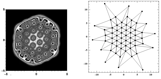
Figure 1. An example of (right): a configuration of zi minimizing the energy (14) for Ω = 0.999,a= 3 andn= 58. (left): density plot of|v|
2.3.
Shape of minimizers and main results
We want to minimize the energy (14) under R
IR2|v|2 = 1, when v ∈ L, that is study (15). A numerical
study [5] consists in writing v(z) = p0Qni=1(z−zi)e−|z|
2/2
and minimize the energy on the locationzi of the zeroes and the degreen. Our numerical observations indicate that vortices are located on a regular triangular lattice in a central region, while the lattice is distorted towards the edges, as illustrated in Figure 1. On the right, we have plotted the ziand on the left |v|. The density plot of|v|shows that the only visible vortices are the central ones in the regular lattice part, the outer ones being in a region of very low density. Our aim is to justify these observations rigorously. In [3, 5], we have constructed an upper bound for the energy inspired by our numerical computations.
2.3.1. Inverted parabola profile
Let us explain the origin of the inverted parabola profile: the minimization of (14) underR
IR2|v|2= 1 without
the constraint of being in the space (5) implies that the minimizer is the inverted parabola
|vmin(r)|2= 2
πR2 0
1− r 2
R2 0
1{r≤R0}, R0=
2a π(1−Ω)
1/4
. (20)
The value of the energy yields a lower bound for ELLL:
ǫmin:=ELLL(vmin)−Ω =2 √
2 3
p
a(1−Ω). (21)
The function vmin does not belong to the space (5), since f =vmine|z|
2/2
is not holomorphic. Nevertheless, a distortion of the vortex lattice inside the space (5) provides a weak star approximation of the inverted parabola
2.3.2. Qualitative properties of minimizers
We are going to rescale the problem. We let R4 = a/(1−Ω), h = 1/R2, and u(r) = Rv(Rr). Then
ELLL(v) = Ω +p
a(1−Ω)Eh
LLL(u) where
ELLLh (u) =
Z
C
|z|2|u|2+1 2|u|
4 dz (22)
wheredz denotes the Lebesgue measuredx1 dx2. We want to minimizeELLLh under the condition thatf(z) =
u(z)e|z|
2
2h is in the Fock Bargmann spaceFh, see [8]:
Fh=
f ∈L2(C, e−|2zh|2dz), s.tf holomorphic
. (23)
The projection of a general functiong(z,z¯) ontoFh is explicit :
Πh(g) = 1
πh
Z
IR2
ezzh′e−
|z′|2
h g(z′,z¯′). (24)
Ifg is a holomorphic function, then an integration by parts indeed yields Πh(g) =g. Using the properties of this space, we are able to derive an equation for the minimizer:
Theorem 2.3. [8] There exists f ∈ Fh such that u(z) = f(z)e−|z|
2/2h
minimizes (22) with kfkFh = 1.
Moreover, f is a solution of the following equation
Πh(|z|2+|f|2e−|z|2/h−µ)f= 0 (25)
whereµ is the Lagrange multiplier coming from the constraint.
The Euler Lagrange equation can be rewritten
zh∂zf +1
2f¯(h∂z)[f
2(2−1.)]
−(µ−h)f = 0, (26)
The operator ¯f(h∂z) being defined as the limit limK→∞PKk=0ak(h∂z)k iff(z) =P∞k=0akzk. This equation allows us to derive that f cannot be a polynomial:
Theorem 2.4. [8] Iff ∈ Fhis such thatu(z) =f(z/ √
h)e−|z|2/2
minimizes (15), thenf has an infinite number
of zeroes.
The proof assumes that f has a finite number of zeroes and derives a contradiction between the degree of the terms in (26).
We would like to prove that the zeroes of the minimizer are arranged on an almost regular lattice. For this purpose, we have to introduce the lattice problem.
2.3.3. The Abrikosov problem
We define a latticeLin the following way:
L= 1
ν (Z⊕τZ), ν∈R ∗
+, τ =τR+iτI ∈C. (27)
The functionsusuch that f(z) =u(z)e|z|2/2h
completely determined by the complex numberτ of the lattice: indeed, the periodicity of|u|imposes the value ofν in terms of handτI. The functionuτ can be expressed in terms of the Theta function according to:
Θ(v, τ) = 1
i
+∞
X
n=−∞
(−1)neiπτ(n+1/2)2e(2n+1)πiv, v∈C.
Such an ansatz was introduced by Abrikosov to minimize the quantity
γ(τ) = −
R
|uτ|4
−
R
|uτ|2
2 (28)
which also arises in the study of superconductors. It turns out that the square (τ =i) and hexagonal lattices (τ=e2iπ/3) are critical points of the functionτ→γ(τ). The fact that the hexagonal lattice is a minimizer was numerically checked by Kleiner, Roth and Autler in [16]. An explicit computation of the quantity γ(τ), with the help of a result by Nonnenmacher and Voros [18] about quantum chaos, provides a complete proof that
τ =e2iπ/3 is the global minimizer:
Theorem 2.5. [8] LetL be a lattice given by its parametersν andτ through (27). If the functionf is entire,
satisfiesf−1({0}) =Lwith simple zeroes, and e
−|z2|h2f(z)
isL-periodic, then the parameter ν and the function
f are determined byτ through:
ν=
r
τI
πh and f(z) =cfτ(z), c∈C ∗
with fτ(z) =e
z2
2hΘ
√τ
I √
πhz, τ
anduτ(z) =e−|z|
2 2h f
τ(z). (29)
The functionfτ(z)solves the equation
Πh
e−|z|
2
h |fτ|2fτ
=λτfτ, inFhs, s <−1, (30)
with λτ=
−
R
|uτ|4
−
R
|uτ|2 = √1
2τI
X
k,ℓ∈Z
e−τIπ|kτ−ℓ|
2
(31)
Moreover, the quantityγ(τ)defined in (28) satisfies
γ(τ) = X k,ℓ∈Z
e−τIπ|kτ−ℓ|
2
. (32)
The complex number τ =j =e2iπ3 , corresponding to the hexagonal lattice, is the unique minimizer of γ(τ) in
the fundamental domain
τ=τR+iτI ∈C, τI >0, |τ| ≥1, − 1
2 ≤τR< 1
2,(τR≤0 if |τ|= 1)
andb=γ(j)∼1.1596.
2.3.4. Upper bound for the energy
We prove that fτ(z)α(z) can be approximated, as h tends to 0, by the function Πh(αfτ) of Fh, which is almost a solution to (25):
Theorem 2.6. [8] Letτ ∈C\R, letα˜∈C0,1
2(C;C) be such thatsupp (˜α)⊂K for some compact setK and
R
|α˜|2= 1. Forf
τ defined by (29), we set
gh ˜
α,τ =kΠh(˜αfτ)k
−1
FhΠh(˜αfτ), and v h ˜
α,τ(z) =gα,τh˜ (z)e−
|z|2
2h . (33)
Then we have
ELLLh vα,τh˜
=
Z
C
|z|2|α˜(z)|2+γ(τ) 2 |α˜(z)|
4
dz+O(h1/4) (34)
whereγ(τ)is given by (28) or (32) andO(h1/4)depends only onkα˜k
C0,1/2, τ andK. Moreover, for anyλ∈C,
Πh|z|2−λ+ Ω2h
vα,τh˜
2
gα,τh˜
= Πh |z|2−λ+γ(τ)|α˜|2
ghα,τ˜
+Rh, (35)
wherekRhkFh ≤C(˜α, τ, λ, K)h1/4, andC(˜α, τ, λ, K)depends only onkα˜kC0,1/2, τ,λandK, and
kvα,τh˜ −αu˜ τkL∞(K)≤Ch1/4.
Let us point out that (35) shows that the projection of the nonlinear term provides the product of the average of|uτ|4, henceγ(τ) times|α˜|2. The difference in the length scales (|uτ|varies on a scale
√
hwhile ˜αvaries on a scale 1) is taken into account to separate the contributions in the product.
In order to approximate a minimizer of (22), we need to pick the optimal function ˜α. Minimizing the right-hand side of (34) with respect toτ and ˜αunder the constraintR
|α˜|2= 1 yields
τ=j and|α˜(z)|2= 1
γ(τ)
r
2γ(τ)
π − |z|
2
!
+
, (36)
where the first equality is a consequence of Theorem 2.5. This provides in particular a test function for the upper bound of the energy (22), and in particular,
ILLL(Ω)−Ω≤ 2 √
2 3
p
ab(1−Ω) (37)
and (34) makes precise the remainder estimate in the upper bound.
With this choice of ˜αandτ, and if in additionλin (35) is such thatλ=p2γ(τ)/π,(35) implies that
Πh|z|2−λ+ Ω2h
vhα,τ˜
2
gα,τh˜
=Oh1/4 in Fh.
In other words,gh ˜
α,τ is a solution to (25) up to an error term of orderh1/4. Moreover, as htends to 0,ghα,τ˜ is very close tofτ(z)˜α(z). This implies that, inside the support of ˜α, the zeroes ofgh
˜
α,τ are located on an almost regular triangular lattice. We do not have much information though, on the zeroes located outside the support of ˜α, the ”invisible vortices”. An open question is to derive that there is a solution to (25) close togh
˜ α,τ, for the specific choice ofτ and ˜αgiven by (36). One may hope to prove such a result by an analogue of a Newton method.
b=γ(j). We expect that reproducing an inverted parabola profile in the space (5) requires a lot of vortices and thus creates a contribution in the energy throughb. But proving that the zeroes of the minimizer (we know by Theorem 2.4 that there is an infinite number) are located on an almost regular lattice seems very difficult and is probably related to similar difficulties in crystallization and sphere packing problems.
3.
Anisotropic case
We go back to the energy (2) and assume thatν6= 0. We address the two-dimensional case only, that is do not enter into the details of the dimensional reduction leading to (6). The energy that we want to minimize is thus
Ean(ψ) =
Z
R2
1 2|∇ψ|
2
−Ω×x·(iψ,∇ψ) +1 2 (1−ν
2)x2
1+ (1 +ν2)x22
|ψ|2+1 2G|ψ|
4 (38)
under theL2constraint, withGequal to 4πN a
0times theL4 norm of the ground state in thezdirection. The critical frequency provides the existence of a small parameterε, with
ε2= 1−ν2−Ω2.
We will see that an anisotropy of the trap can drastically change the picture in the fast rotation regime, that is smallε.
We would like to perform the same steps as in the isotropic case, that is find new coordinates (equivalent of the LLL) where the energy gets simplified and then study this reduced energy in order to understand the vortex behaviour. This is performed in [6, 7] and uses the diagonalization of the quadratic form in a simplectic basis, as we will see below, to find the reduced energy
ELLL(ψ) =
Z
R2
1 2(ε
2x2
1+κ2x22)|ψ|2+
G
2|ψ|
4 (39)
withκ2∼(ν2+ε2/2)(2−ν2)
(1−ν2) asεtends to 0. ELLL is minimized on the spaceL given by (5). Thus, we are interested in the following problem
I(ε, κ) = inf
ELLL(ψ), ψ∈L,
Z
IR2|
ψ|2= 1
. (40)
Asεtends to 0, the condensate expands in thex1direction. In thex2 direction, according to the values ofε andν, either the condensate expands (inverted parabola profile) or stays bounded. Indeed, the minimization without the holomorphy constraint yields
|ψ|2= 2
πR1R2 (1− x
2 1
R2 1
− x 2 2
R2 2
), whereR1=
2Gκ
πε3
1/4
, R2=
2Gε
πκ3
1/4
.
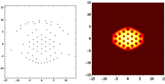
There are 2 regimes: • ε1/3 >> κ: R
2 → ∞. Numerical simulations (figure 2) show a triangular vortex lattice with an inverted parabola profile. The behaviour is similar to the isotropic case except that the inverted parabolaαtakes into account the anisotropy,f = Π(α(z)fτ(z)) is an approximate solution of the equation.
• ε1/3<< κ: R
2→0. Numerical simulations (figure 3) show that the behaviour is an inverted parabola in thex1 direction and a fixed gaussian in thex2 direction. The shrinking of the condensate in thex2direction is not allowed in the lowest Landau level because the operatorx2
-10 0 10
-15 -5 5
-10 0 10
-5 5 15
Figure 2. Plot of the zeroes of the minimizer (left) and the density (right) for ε2 = 0.002,
ν= 0.0316. Triangular vortex lattice in an anisotropic trap.
-40 -30 -20 -10 0 10 20 30 40 -40
-30 -20 -10 0 10 20 30 40
Figure 3. Plot of the zeroes of the minimizer (left) and the density (right) for ε2 = 0.002,
ν= 0.06. No vortex in the visible region.
3.1.
Reduction to an LLL energy
In this section, we sketch the computations which allow to reduceEan toELLLand the space L. We define the quadratic form corresponding to the linear terms in the energy:
Q(x1, x2, ξ1, ξ2) =ξ12+ξ22+ (1−ν2)x21+ (1 +ν2)x22−2Ω(x1ξ2−x2ξ1), (41)
We consider the phase space IR2x×IR2ξ with the symplectic formσ, which is a bilinear alternate form given by
σ (x, ξ); (y, η)
=ξ·y−η·x=< σXY >, X =
x ξ
, Y =
y η
, σ=
0 I2 −I2 0
, (42)
where the formσis identified with the 4×4 matrix above.
where
µ2
1= 1 + Ω2−
p
ν4+ 4Ω2, µ2
2= 1 + Ω2+
p
ν4+ 4Ω2. We define α = √ν4+ 4Ω2, β
1 = (2Ωµ1)/(α−2Ω2+ν2), β2 = (2Ωµ2)/(α+ 2Ω2+ν2), γ = (2α)/Ω, λ21 = (α−2Ω2+ν2)/(2α), λ2
2 = (α+ 2Ω2+ν2)/2α, d= (γλ1λ2)/2, c= (λ21+λ22)/2λ1λ2.Then computations lead to the following diagonalization ofQ:
Q= 1 2
a†1a1+a1a†1
+1 2
a†2a2+a2a†2
where
a2=
µ2 √
2 −iλ1d
−1∂
x1+cλ1x2
+√i
2 −iλ2∂x2− dλ
−1
1 −λ2cdx1,
and
a1=
µ1 √
2 −iλ2d
−1∂
x2+cλ2x1
+√i
2 (λ1cd−dλ
−1
2 )x2−iλ1∂x1
.
We have: ha2, a†2
i
=µ2,
h
a1, a†1
i
=µ1, and all other commutators vanish. Since µ1 < µ2, the LLL is then
defined by a2ψ= 0, that is f(x+iβ2y)e
h
− 1 8β2
“2α−ν2
Ω x
2+2α+ν2
Ω (β2y)2 ”i
−iν2
4Ωxy, with f analytic. In the LLL, we
have< Qψ, ψ >= 12 <(a†1a1+a1a†1ψ, ψ >+µ22 < ψ, ψ > . a1, a2, a
†
1, a
†
2 [13] and get, ifψ∈LLL,
< Qψ, ψ >= µ2 2 −
µ1 4
β1β2+ 1
β1β2
+γ 4 Z R2
µ1β1x21+
µ1
β1
x22
|ψ|2dx1dx2. (43)
It is always possible to change the analytic functionf(ξ) intof(ξ) exp(−δξ2) in the above definition of the LLL, since exp(−δξ2) is an analytic function of ξ. Hence, for δ =ν2/(8Ωβ
2), we find the alternative definition of the LLL, which, after rescaling by β2 yields the same LLL as in the isotropic case, that is the spaceL. This definition is equivalent to the one given by Fetter in [13]. Moreover (43) provides (39) with κ2 =γµ
1/2β1 and sinceγµ1β1∼2ε2,β2∼
p
(1−ν2)/(1−ν2/2) andγ∼(4−2ν2)/√1−ν2.
The rest of this section is dedicated to the minimization of (38), which yields two different cases according to the behaviour ofκ/ε1/3.
3.2.
Weakly anisotropic case
In this section, we assume that
ε≤κ≪ε1/3 . (44)
This case is similar to the isotropic case and we derive similar results to the previous section, namely an upper bound given by the Theta function but we lack a good lower bound. The isotropic case is recovered by assuming
κ=ε.
Theorem 3.1. [7] If (44)is satisfied, and if ε→0, then we have
2 3
r
2Gεκ
π < I(ε, κ)≤
2 3
r
2Gbεκ π +O
√
εκ
κ3
ε
1/8!
, (45)
where b =γ(j)≈1.1596 is given by the Abrikosov problem. Moreover, the following function gives the upper
bound in (45):
v= ΠL(uτα), (46)
whereuτ is defined by (29)withh= 1, and
α(x)2= 2
π√bR1R2
1− x 2 1 √ bR2 1 − x 2 2 √ bR2 2 ! +
, R1=
2Gκ πε3
1/4
, R2=
2Gε πκ3
1/4
We point out that the lower bound does not include b. We expect the energy asymptotics to match the right-hand side of (45). Thus, the lower bound is not optimal. This is confirmed by numerics.
3.3.
Very fast rotation
In the case where the rotation is fast enough with respect to the anisotropy in the sense that
κ≫ε1/3 (47)
we have found a regime unknown by physicists where vortices disappear and the problem can be reduced in fact to a 1D energy.
Theorem 3.2. [7] Assume (47). Then, we have
I(ε, κ) = κ 2
8π+Jε
2/3+oε2/3, (48)
asε→0, where
J = inf
Z
IR 1 2t
2p(t)2+G 2
Z
IR
p(t)4, p∈L2(IR)∩L4(IR),
Z
IR
p2= 1
. (49)
In addition, ifuis a minimizer of I(ε, κ), then
1
ε1/3
u
x1
ε2/3, x2
−→2
1/4e−πx2 2p(x
1), (50)
in L2(IR2)
∩L4(IR2), wherepis the minimizer of J.
This is due to the fact that the operatorx2
2is bounded below by a constant in the LLL. The ground state of the operatorx2
2is
u(x1, x2) =
γβ
2π
1/4
exp
−γβ4 x22+i
γ
4x1x2
(51)
and every function in the LLL cannot be more localized in the x2 direction than (51). This provides an upper bound. The projection onto the space of separate variables inx1andx2is enough to provide the suitable lower bound.
3.4.
Open questions
The missing information correspond to the intermediate regime whereε1/3/κconverges to some limitλ. We expect that the extension in the x2 direction depends on λ and wonder whether the condensate has a finite number of vortex lines.
Numerical simulations are still to be performed.
References
[1] Abo-Shaeer JR, Raman C, Vogels JM, Ketterle W, Observation of Vortex Lattices in Bose-Einstein Condensates (2001) Science
292, 476-479.
[2] Aftalion A, Vortices in Bose Einstein condensates, Progress in Nonlinear Differential Equations and their Applications, Vol.67 Birkh¨auser Boston, Inc., Boston, MA, (2006).
[3] Aftalion A, Blanc X, Vortex lattices in rotating Bose Einstein condensates, (2006), SIAM J. Math. Anal., Vol 38, p 874. [4] Aftalion A, Blanc X, Reduced energy functionals for a three dimensional fast rotating Bose Einstein condensates, (2008), Ann.
I.H.P., Vol. 25, 339-356.
[6] Aftalion A, Blanc X, Lerner N, Fast rotating condensates in an asymmetric harmonic trap, (2008), condmat-0804.0971. [7] Aftalion A, Blanc X, Lerner N, (2008), in preparation.
[8] Aftalion A, Blanc X, Nier F, Lowest Landau Level for Bose Einstein condensates and Bargmann transform, (2006) J. Func. Anal. Vol 241, pp 661-702.
[9] Bretin V, Stock S, Seurin Y, Dalibard J, Fast Rotation of a Bose-Einstein Condensate Phys. Rev. Lett.92, 050403 (2004). [10] Cohen-Tannoudji CN, in: Les Prix Nobel 1997 (The Nobel Foundation, Stockholm, 1998), pp. 87-108, Reprinted in: Rev.
Mod. Phys. 70:707-719.
[11] Cooper NR, Komineas S, Read N,Vortex lattices in the lowest Landau level for confined Bose-Einstein condensates, Phys. Rev. A70, 033604 (2004).
[12] Cornell EA, Wieman CE,Bose-Einstein condensation in a dilute gas, the first 70 years and some recent experiments, in: Les Prix Nobel 2001 (The Nobel Foundation, Stockholm, 2002), pp. 87-108, Reprinted in: Rev. Mod. Phys. 74, 875-893; Cem. Phys. Cem.3, 476-493 (2002).
[13] Fetter AL, Lowest-Landau-level description of a Bose-Einstein condensate in a rapidly rotating anisotropic trap, Phys. Rev. A75, 013620 (2007).
[14] Ho TL, Bose-Einstein Condensates with Large Number of Vortices, Phys. Rev. Lett.87060403 (2001).
[15] Ketterle W,When atoms behave as waves: Bose-Einstein condensation and the atom laser, in: Les Prix Nobel 2001 (The Nobel Foundation, Stockholm, 2002), pp. 118-154, Reprinted in: Rev. Mod. Phys.74, 1131-1151 (2002); Chem. Phys. Chem.
3, 736-753 (2002)
[16] Kleiner WH, Roth LM, Autler SH, Bulk Solution of Ginzburg-Landau Equations for Type II Superconductors: Upper Critical Field Region, Phys. Rev.133, A1226, (1964).
[17] Madison K, Chevy F, Bretin V, Dalibard J, Vortex Formation in a Stirred Bose-Einstein Condensate, (2000) Phys. Rev. Lett.,
84, 806.
[18] Nonnenmacher S, Voros A, Chaotic Eigenfunctions in Phase Space, J. Stat. Phys. 92, 431-518 (1998). [19] Pethick CJ, Smith H, (2002) Bose Einstein condensation in dilute gases, Cambridge University Press.
[20] Pitaevskii L, Stringari S, (2003) Bose Einstein condensation, International series of monographs on physics, 116, Oxford Science Publications.
[21] Rosenbuch P, Bretin V, Dalibard J, Dynamics of a single vortex line in a Bose-Einstein condensate (2002) Phys. Rev. Lett.
89, 200403.
[22] Stock S, Bretin V, Chevy F, Dalibard J, Shape oscillation of a rotating Bose-Einstein condensate, Europhys.Lett. 65594 (2004).