A coupled well-balanced and random sampling scheme for computing bubble oscillations*

(1)

Fédération Denis Poisson (Orléans-Tours) et E. Trélat (UPMC), Editors

A COUPLED WELL-BALANCED AND RANDOM SAMPLING SCHEME FOR

COMPUTING BUBBLE OSCILLATIONS

∗

Philippe Helluy

1

and Jonathan Jung

2

Abstract. We propose a finite volume scheme to study the oscillations of a spherical bubble of gas in a liquid phase. Spherical symmetry implies a geometric source term in the Euler equations. Our scheme satisfies the well-balanced property. It is based on the VFRoe approach. In order to avoid spurious pressure oscillations, the well-balanced approach is coupled with an ALE (Arbitrary Lagrangian Eulerian) technique at the interface and a random sampling remap.

Résumé. Nous proposons un schéma de volumes finis pour étudier les oscillations d’une bulle sphérique de gaz dans l’eau. La symétrie sphérique fait apparaitre un terme source géométrique dans les équations d’Euler. Notre schéma est basé sur une approche VFRoe et préserve les états stationnaires. Pour éviter les oscillations de pression, l’approche well-balanced est couplée avec une approche ALE (Arbitrary Lagrangian Eulerian), et une étape de projection basée sur un échantillonage aléatoire.

Introduction

We want study the behavior of a spherical bubble of gas in a liquid phase. Note that the equations will be the same as in the case of flows in variable cross-section. Classical finite volume solvers generally have a bad precision for solving two-fluid interfaces or flows in varying cross-section ducts. Several cures have been developed for improving the precision.

• For cross-section ducts, the well-balanced approach of Greenberg and Leroux [5] (see also [6, 10]) is an

efficient tool to improve the precision.

• For two-fluid flows the pressure oscillations phenomenon (see [2,8] for instance) can be cured by a recent

tool developed in [1, 4]. It is based on an ALE (Arbitrary Lagrangian Eulerian) scheme followed by a random sampling projection step.

In this paper, we show that it is possible to mix the two approaches in order to design an efficient scheme for computing the collapse of a spherical bubble of gas in a liquid phase.

1. Model

1.1. Equations

To study a spherical bubble of gas in a liquid phase we consider the 3D-Euler equations. We assume that the

flow is invariant under rotation. We notexthe space variable along the radius of the bubble andtthe time (see

∗_{This work has been partly supported by a PICS CNRS grant.}

1 _{IRMA, University of Strasbourg; [email protected]} 2 _{IRMA, University of Strasbourg; [email protected].}

c

EDP Sciences, SMAI 2012

(2)

Figure 1(a)). With the spherical symmetry the unknowns are the density ρ, the radial velocityu, the internal

energye and the fraction of gasϕ and they depend only on (x, t). We can put the 3D-Euler equations in the

following form

∂t(Aρ) +∂x(Aρu) = 0, (1)

∂t(Aρu) +∂x(A(ρu2+p)) = p∂xA, (2)

∂t(AρE) +∂x(A(ρE+p)u) = 0, (3)

∂t(Aρϕ) +∂x(Aρϕu) = 0, (4)

∂tA = 0, (5)

where

p=p(ρ, e, ϕ), E=e+u

2

2 , (6)

andA(x) =x2 _{appears because of spherical symmetry. Without loss of generality, in this paper we consider a}

stiffened gas pressure law (see [11] and included references)

p(ρ, e, ϕ) = (γ(ϕ)−1)ρe−γ(ϕ)π(ϕ), (7)

where (γ, π)(ϕ= 1) = (γgas, πgas) and (γ, π)(ϕ= 0) = (γliq, πliq).

We can also put the system (1)-(5) in the non-conservative form

∂tW +∂xF(W)−S(W)∂xA= 0, (8)

where

W = (Aρ, Aρu, AρE, Aρϕ, A)T, (9)

F(W) = (Aρu, A(ρu2+p), A(ρE+p)u, Aρϕu,0)T, (10)

S∂xA = (0, p∂xA,0,0,0). (11)

We define the vector of primitive variables

Y = (ρ, u, p, ϕ, A)T. (12)

We define also the following quantities

Q= mass flow rate =ρAu, s= entropy = (p+π(ϕ))ρ−γ(ϕ), (13)

h= enthalpy =e+p

ρ, H = total enthalpy =h+

u2

2 . (14)

The sound speedc satisfies

c2=pρ=ρhρ. (15)

1.2. Properties

Proposition 1.1. The jacobian matrix of the non conservative system (8) admits five real eigenvalues

λ0= 0, λ1=u−c, λ2=λ3=u, λ4=u+c. (16)

However, the system may be resonant (whenλ0=λ1 orλ0=λ4.)

The quantitiesϕ,s,QandH are independent Riemann invariants of the stationary waveλ0.

(3)

2. A well-balanced two-fluid ALE solver

2.1. Principe

The objective of our algorithm is to determine the behavior of a spherical gas bubble. For computing the gas-liquid interface, we propose to mix front-tracking and front-capturing approaches. First, we apply Arbitrary Lagrangian Eulerian (ALE) ideas: at the interface between gas and water we use a Lagrangian approach. Elsewhere, we use an Eulerian scheme.

We divide the domain Ω intoN cells Ωi=]xi−1/2, xi+1/2[ centered onxi.We denote byτ the time step and

by ∆xi=xi+1/2−xi−1/2 the size of cell i. The area of the sectionAis approximated by a piecewise constant

function,A=Ai in cell Ωi.

The boundaryxn

i+1/2 can move at the velocity of the fluidvni+1/2 between timetn andtn+1, thus we have

xn_i₊₁+1_/,₂−=xi+1/2+τ vni+1/2 (17)

where at the gas-liquid interface (i.e ϕn

i 6=ϕni+1) we have vni+1/26= 0, everywhere else we havevin+1/2= 0.

Suppose that at time tn we know an approximation Wn _{of the exact solution} _W_{. The approximation is}

constant on each cell

W(tn, x)≃Wn(x) =Win, x∈Ωi. (18)

AsAis constant on each cell, the integration of the non-conservative system (8) on the quadrilateral space-time

Q={(x, t)∈R2|tn< t < tn+1, xn_i−1

2 +t×v

n

i−1/2< x < xni+1

2 +t×v

n i+1/2}

= [

tn<t<tn+1 ]xn_i−1

2 +t×v

n i−1/2;x

n i+1

2 +t×v

n

i+1/2[×{t}

gives

Z Z

Q

∂tW +∂xF(W) = 0. (19)

To simplify the formula, we define a discontinuous Arbitrary Lagrangian Eulerian (ALE) numerical flux

F(WL, WR, v±

) :=F(W(WL, WR, v±

))−vW(WL, WR, v±

)) (20)

where W(WL, WR, v±

) = WRiemann(WL, WR,x_t =v±

). We cannot confuse the fluxes denoted by F because

they do not depend on the same number of variables. By applying Stokes’ formula to (19), we have

• ifvn

i+1/2≤0 andv

n

i−1/2≥0

∆xni+1,−W

n+1,−

i −∆xiWin+τ(F(Win, Win+1, v n,−

i+1/2)−F(W n

i−1, Win, v n,+

i−1/2)) = 0, (21)

• In order to take into account the variable section, we also have to make the following corrections

– ifvn

i+1/2>0, we add the following term on the left side of the equation above

τ(F(Win, Wmoyn ,0

−

)−F(Win, Wmoyn ,0+)), (22)

whereWn

moy=W(Ymoyn = (ρni, uni, pni, ϕni, Ani+1)), – ifvn

i−1/2<0, we add

τ(F(Wn

moy, Win,0

−

)−F(Wn

moy, Win,0+)). (23)

whereWn

(4)

In this equality, the time stepτ satisfies a CFL condition

τ ≤max i

△xi

|ui|+ci. (24)

To updateW_in+1,−, we have to computeF(WL, WR, v±_{). To do that, we need to:}

• precise how we choose the ALE velocityv,

• explain how we computeF(WL, WR, v±

) for a given ALE velocityv.

2.2. ALE velocity

We have now to express the velocity v that depends on the data WL and WR. The idea is to use the

well-balanced scheme everywhere except at the interface between the two fluids. At this interface we use the

Lagrange flux. When our initial data satisfyϕ∈ {0,1}, the algorithm reads:

• if we are not at the interface, i.e. if ϕL =ϕR, we takev= 0,

• if we are at the interface, i.e. if ϕL 6= ϕR. We use an exact Riemann solver of variable (ρ, u, p, ϕ)

to compute the pressure and the velocity at the contact discontinuity, which presents no jump at this

discontinuity. We thus denote by u∗

(WL, WR) and p∗

(WL, WR) the velocity and the pressure at the contact. We take

v=u∗(WL, WR), (25)

A∗ =

(

AL , if v <0

AR , if v >0. (26)

The numerical flux ALE becomes lagrangian and takes the form

F(WL, WR, v±

) = (0, A∗

p∗

, A∗

u∗

p∗

,0,−A∗

u∗

)T. (27)

2.3. Computing

W

(

W

L

, W

R

,

0

±

)

As the invariants of Riemann associated to the stationary wave areϕ,s,Q,H (prop 1.1), the idea is to use a

VFRoe ncv solver (see [3]) in the variablesZ = (A, ϕ, s, Q, H) to compute the interface statesW(WL, WR,0±

). We proceed as follows. For regular solutions, system (1)-(5) may be rewritten in the non-conservative form

∂tZ+C(Z)∂xZ= 0 (28)

where

C(Z)=



      

0 0 0 0 0

0 u 0 0 0

0 0 u 0 0

0 A(∂ϕp−ρ∂ϕh) A(∂sp−ρ∂sh) u ρA

0 u

ρ∂ϕp

u ρ∂sp

c2 ρA u



      

(29)

that admits 5 real eigenvalues

λ0= 0, λ1=u−c, λ2=λ3=u, λ4=u+c. (30)

Now, we want to solve

∂tZ+C(Z)∂xZ= 0, (31)

with the initial data

Z(x,0) =

(

Z(WL) , x <0,

(5)

• We approximateC(Z) at ˆZ =Z(YL+YR

2 ) and we solve the linear Riemann problem

∂tZ+C( ˆZ)∂xZ= 0,

with the same initial datas.

• We obtainZ(WL, WR,0±_).

• We go back to W(WL, WR,0±_{). It appears that this change of variable is not always invertible. We}

deal with this difficulty as in [6].

The VFRoe ncv scheme without entropy correction can approach incorrect rarefaction waves crossing the

interface x = 0 and thus authorizes in these points non physical shocks. To solve this problem, we use the

following entropy correction presented in [7]:

Definition 2.1. Ifλk(Wn

i )≤0≤λk(Win+1) in a non linear k-field, then the numerical fluxF is replaced by

G(Win, Win+1,0

±

) = F(Win, Win+1,0

± )

− min

k (|λk(W n

i )|,|λk(Win+1)|)(Win+1−Win)/2.

2.4. Glimm remap

We go back to the original Euler grid by the Glimm procedure. We construct a sequence of pseudo-random

numbers ωn∈[0,1[.In practice, we consider the (5,3) van der Corput sequence [1]. According to this number

we take

Win+1=



 

 

Win−+11,−, if ωn< ∆τximax(vin−1/2,0), W_in+1,−, if τ

∆ximax(v n

i−1/2,0)≤ωn≤1 + ∆τximin(v n i+1/2,0), Win+1+1,−, if ωn>1 + ∆τximin(vin+1/2,0).

(33)

2.5. Properties of the scheme

The constructed scheme has many interesting properties:

• it is well-balanced in the sense that it preserves exactly all stationary states (i.e. initial data for which

the quantitiesϕ, s, Q, H are constant);

• for a flow in a duct with constant cross-section ducts, it computes exactly the contact discontinuities,

with no smearing at the interface;

• if at the initial time the mass fraction is in{0,1}, then this property is exactly preserved at any time.

For detailed proofs, we refer to [1, 6]. Some other subtleties are given in the same references. For instance, the

change of variablesZ=Z(W) is not always invertible, that implies to define a special procedure for constructing

completely rigorously the well-balanced VFRoe solver.

3. Numerical result: Implosion of a bubble

We simulate the collapse of a spherical bubble of vapor in liquid water. In this case we recall thatA(x) =x2_.

We assume that the initial radius of the bubble is Rmax= 0,7469×10−4_{. The computation is carried out on}

Ω = [0; 20×Rmax] with approximativelyN= 15000 cells. Initial datas are the following:

Quantity Left Right

ρ(kg.m−3₎ ₀_.₉₂ ₁₀₀₀ u(m.s−1₎ ₀ ₀

p(P a) 72567.68 105

ϕ 1 0

γ 1.4 3

(6)

Water

Gas x

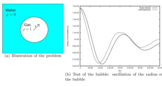
(a) Illustration of the problem

6.6e-05 6.7e-05 6.8e-05 6.9e-05 7e-05 7.1e-05 7.2e-05 7.3e-05 7.4e-05 7.5e-05

0 5e-06 1e-05 1.5e-05 2e-05 2.5e-05 3e-05 3.5e-05 4e-05

Radius of the bubble (m)

t(s)

’Keller-Miksis’ ’Well-balanced’

(b) Test of the bubble: oscillation of the radius of the bubble

Figure 1

The amplitude of the oscillations of the radius obtained with our scheme (see Figure 1(b)) is comparable with those obtained with the model of Keller-Miksis (see [9]). Let us remind that the model of Keller-Miksis is an estimate of the real flow. It must be considered as a reference solution but not as an exact solution.

4. Conclusion

We have constructed and validated a new one order scheme to compute the oscillation of a spherical bubble

in a liquid phase. The smooth functionA is approximated by a piecewise constant function. Our scheme relies

on two ingredients:

• a well-balanced approach for dealing with the varying cross-section;

• a Lagrange plus remap technique in order to avoid pressure oscillations at the interface. The random

sampling remap ensures that the interface is not diffused at all.

Our scheme can also be applied to flows in a nozzle with variable cross-section.

References

[1] M. Bachmann, P. Helluy, H. Mathis, S. Mueller, Random sampling remap for compressible two-phase flows, Preprint HAL http://hal.archives-ouvertes.fr/hal-00546919/fr/.

[2] T. Barberon, P. Helluy, S. Rouy, Practical computation of axisymmetrical multifluid flows, Int. J. Finite Vol. 1, no. 1, 34 pp, 2004.

[3] T. Buffard, T. Gallouet, J.-M. H´erard. A sequel to a rough Godunov scheme: application to real gases, Computers and Fluids, vol. 29, pp. 813-847, 2000.

[4] C. Chalons, F. Coquel. Computing material fronts with a Lagrange-Projection approach. HYP2010 Proc. http://hal.archives-ouvertes.fr/hal-00548938/fr/.

[5] J.-M. Greenberg, A.Y., Leroux. A well balanced scheme for the numerical processing of source terms in hyperbolic equations, SIAM J. Num. Anal., vol. 33 (1), pp. 1-16, 1996.

[6] P. Helluy, J.-M. H´erard, H. Mathis. A Well- Balanced Approximate Riemann Solver for Variable Cross- Section Compressible Flows. AIAA-2009-3540. 19th AIAA Computational Fluid Dynamics. June 2009.

[7] P. Helluy, J.-M H´erard, H. Mathis, S. Mueller. A simple parameter-free entropy correction for approximate Riemann solvers, Comptes rendus M´ecanique, 2010.

[8] S. Karni. Multicomponent flow calculations by a consistent primitive algorithm. J. Comput. Phys. 112, no. 1, pp. 31-43, 1994. [9] B. Keller, M.Miksis. Bubble oscillations of large amplitude, J. Acoust. Soc. Am., 68(2), pp. 628-633, 1980.

[10] D. Kroner, M.-D. Thanh. Numerical solution to compressible flows in a nozzle with variable cross-section, SIAM J. Numer. Anal., vol. 43(2), pp. 796-824, 2006.