Weighted Negative Binomial-Poisson Lindley with Application to Genetic Data

(1)

Original Article

Weighted negative binomial-Poisson Lindley with application to genetic data

Hossein Zamani1*_{, Noriszura Ismail}2_{, Marzieh Shekari}1

1 _{Department of Mathematics and Statistics, Faculty of Science, University of Hormozgan, Bandarabbas,}_Iran 2_{School of Mathematical Sciences, Universiti Kebangsaan Malaysia}_,_Selangor,_Malaysia

ARTICLE INFO ABSTRACT

Received 18.12.2017 Revised 27.12.2017 Accepted 12.03.2018

Background & Aim: Mixed Poisson and mixed negative binomial distributions have been considered as alternatives for fitting count data with over-dispersion. This study introduces a new discrete distribution which is a weighted version of Poisson-Lindley distribution.

Methods & Materials: The weighted distribution is obtained using the negative binomial weight function and can be fitted to count data with over-dispersion. The p.m.f., p.g.f. and simulation procedure of the new weighted distribution, namely weighted negative binomial-Poisson-Lindley (WNBPL), are provided. The maximum likelihood method for parameters estimation is also presented.

Results: The WNBPL distribution is fitted to several datasets, related to genetics and compared with the Poison distribution. The goodness of fit test shows that the WNBPL can be a useful tool for modeling genetics datasets.

Conclusion: This paper introduces a new weighted Poisson-Lindley distribution which is obtained using negative binomial weight function and can be used for fitting over-dispersed count data. The p.m.f., p.g.f. and simulation procedure are provided for the new weighted distribution, namely the weighted negative binomial-Poisson Lindley (WNBPL) to better inform parents from possible time of occurrence reflux and treatment strategies.

Key words: Weighted distribution; Poisson distribution; Discrete distribution; Mixed distribution, Mixed Poisson

Introduction

Mixed Poisson and mixed negative binomial distributions have been considered as alternatives for fitting count data with over-dispersion (1-5). Several examples of mixed Poisson and mixed negative binomial distributions can be found in several statistical literatures (6-23), such as negative binomial which is obtained as a mixture of Poisson and gamma, Poisson-Lindley (6, 18), Poisson-lognormal (1), Poisson-inverse Gaussian (24, 25), negative binomial-Pareto (12), negative inverse Gaussian (7), negative binomial-Lindley (26, 11), Poisson-exponential (2), Poisson-weighted exponential (27), two parameter Lindley (19) and Poisson-Janardan distributions (20).

Besides mixed distributions, weighted distributions have also been considered as

alternatives for fitting count data with over-dispersion, and can be generally obtained by multiplying a count distribution with a weight function. To derive a new weighted distribution, let X be a count random variable with p.m.f.

)

(

X

k

P

=

, where

k

∈

N

₀

=

{

0

,

1

,

2

,...}

. Let

( )

k

ω

be a non-negative function on

N

₀ having a finite expectation

0

( ( )) _k ( ) ( )

E _ω X =



∞₌ _ω k P X =k < ∞, where the weight function

ω

( )

k

can be used to adjust the probability when X =k occur. Thus, the weighted version of r.v . X , which is the realization of count r.v. Y, has the following p.m.f:

0

( ) ( )

( ) ( ; ) ,

( ( ))

k P X k

P Y k p k k N

E X

ω θ

ω

=

= = = ∈ . (1)

The most popular weighted count distributions are the weighted Poisson (WP) distributions which are obtained when the initial count r.v., X , follows a Poisson distribution. The initial concept of WP distribution was introduced in (16), which lead to several more _____________________________________________________

* Corresponding Author: Hossein Zamani, Postal Address: Department of Mathematics and Statistics, Faculty of Science, University of Hormozgan, Bandarabbas, Iran.

(2)

recent and different types of WP distributions derived and analyzed in other studies. Examples of a more recent WP distributions can be found in (3,17, 22).

In recent studies, some authors used particulars weights for deriving new versions of weighted distributions. Such examples can be found in(13) who used the Poisson weight function

ω

( ; )

k

ϕ ϕ

=

k

e

−ϕ

( !)

k

−1_{, Kokonendji} (10) who utilized the binomial weight function

( ; ) 1 (1

k

)

k

ω

ϕ

= − −

ϕ

, and the negative

binomial weight function

1

( ; )

k

ϕ

ω

ϕ

=





+ −









which was applied by

(8). A more detailed study of weighted distributions and weight functions can be found in (15).

The objective of this study is to introduce a new discrete weighted distribution based on the Poisson-Lindley distribution. The weighted distribution, namely the weighted negative binomial-Poisson Lindley (WNBPL), is weighted with the negative binomial weight function and can be used as an alternative for fitting count data with over-dispersion. The rest of this paper is organized as follows. Section 2 provides the p.m.f., p.g.f. and simulation procedure for the WNBPL. Maximum likelihood method for parameters estimation is provided in Section 3. Several numerical illustrations are provided in Section 4, where the Poisson, and WNBPL are fitted to a few datasets.

Methods

Weighted Poisson-Lindley Negative Binomial (WPLN)

P.m.f., p.g.f., mean, and variance: Assume r.v.

Y

|

λ

follows Poisson distribution with p.m.f:

( | )

,

0,1, 2,...

!

y

e

p y

y

λ

=

−

=

, (2)

and parameter

λ

is distributed as Lindley with parameter

θ

:

2

( )

(1

)

0

1

f

λ

θ

λ

e

θλ

λ

θ

−

=

+

>

+

. (3)

The Poisson-Lindley (PL) distribution is obtained by mixing the Poisson and Lindley distributions, and the p.m.f. is:

2

3

(

2)

( )

,

0,1, 2,3...

(1

)

y

p y

θ

y

θ

+

+ +

=

+

, (4)

with mean and variance: 3 2

2 2

2 4 6 2

( ) , ( )

( 1) ( 1)

E Y θ Var Y θ θ θ

θ θ θ θ

+ + + +

= =

+ + .

Using

p 1 1= +

θ for re-parameterization, the PL p.m.f. in (4) can be re-written as:

2

( ) (1 ) y(1 ) 0,1,2,3,... p y = −p p + +p py y =

(5)

A new discrete distribution can be easily obtained by inserting the negative binomial

weight function

( ; )

k r

r k

1

k

ω

=





+ −









and the

PL p.m.f. (5) into the weighted equation in (1). The new distribution, namely the WNBPL, has the following p.m.f:

r 1

2 2

r 1 (1 ) (1 )

( ) ( ) , 0,1, 2,..., 0 1

(1 r ) k

k p p p pk

P Y k p k k p

k p p

+ + −

  − + +

= = =  ₋ ₊ = < <

 

(6)

with mean and variance:

2 2

2

2 2 2 2

r (r 1)

1 r 1

(r )( 1) (r 1)

(1 r ) (1 )

p p p p

p p p

p p p p p

p p p

μ

σ

− − +

= +

+ − −

− − + +

= +

+ − −

(7)

The p.g.f. can be obtained in a closed form, and is given by:

1 2 2

2 2

(1 r ) (1 ) 1

( ) ( )

(1 r ) 1

r Y

Y

p t p t p t p

G t E t

p p pt

+

 

− + + − −

= = ₋ ₊  ₋ 

 

. (8)

Over-dispersion

In statistics, cases of over-dispersion can be determined by comparing the mean and variance, where a distribution is known to be over-dispersed if the variance is greater than the mean. For WNBPL, the variance and mean can be written as:

2 2 2 2

2

2 2 2 2

(r 1) (r )

(1 ) (1 r )

p p p p

p p p

σ

− =

μ

+ − − −

− + − ,

so that we can determine whether the term

2 2 2

) 1

(

) (

p rp

p p rp

− +

−

(3)

pand

r

. If

2 2 2

) 1

(

) (

p rp

p p rp

− +

−

− _{is less than one,}

then 2 2

) 1 (

p r p

−

+ _{is greater than one, indicating that}

μ

σ2− _{is greater than zero. Therefore, the}

variance of WNBPL is greater than the mean, and the distribution can be used to handle over-dispersed count data.

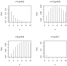
Figure 1 shows the p.m.f. of WNBPL for different values of

( , )

r p

. The graphs indicate that the distribution can be considered as an alternative for over-dispersed count data.

Random data generation

P.m.f. (6) indicates that

WNBPL

(

r

,

p

)

is a mixture of negative binomial distributions, which can be written as:

) 1 , 1 ( 1

) 1 , ( 1

1 )

( ₂ ₂

2

2 2

2

p r NB rp p

rp p

r NB rp p

p k

p ₊ ₋

+ − + − +

− −

= .

Therefore, the

WNBPL

(

r

,

p

)

random samples can be generated via the weighted negative binomial approach.

We analyze the performance of ML estimates of

WNBPL

(

r

,

p

)

based on 1000 simulations. The average estimators, average mean square

errors and average standard errors of the ML estimates for several sample sizes,

n

, and several initial values

(

r

,

p

)

, are provided in Table 1. The results show that increasing the sample size is an effective way of decreasing the standard errors of parameters. As shown in this table, the MSEs decrease when the sample size increase, and thus, suggesting the consistency of the proposed model.

Parameter Estimation

Let

Y

₁

,

Y

₂

,...,

Y

_n be an i.i.d. random sample drawn from WNBPL distribution, with observed values

k

₁

,

k

₂

,...,

k

_n. The log-likelihood is:

1 1

2 2

1

ln ( , ) ( , ) ( 1) ln(1 ) ln ln(1 )

1

ln(1 )

n n

i i

n i

i i

L r p r p n r p k p p pk

r k n p rp

k

= =

=

= = + − + + + +

+ −

 

− − + +  

 

 





By partially differentiating the log-likelihood with respect to p and

r

, we obtained:

2 2 1

1

( , ) ( 1) 2 ( 1)

1 1 1

n

i

i i

k

r p n r nk np r

p p p ₌ p pk p rp

+

∂ _{= −} + ₊ ₊ ₋ −

∂ −



+ + − +



Figure 1. P.m.f. of WNBPLN distribution for different values of

( , )

r p

0 2 4 6 8 10

0.

00

.1

0.

20

.3

r=1,p=0.5

k

PL

N

0 2 4 6 8 10

0.

03

0.

05

0.

07

r=1.5,p=0.8

k

PL

N

0 2 4 6 8 10

0.

01

0.

03

0.

05

r=2,p=0.8

k

PL

N

0 2 4 6 8 10

0.

0

0.

4

0.

8

r=1,p=0.1

k

PL

(4)

2

2 2

1

( , ) _ln(1 ₎ _ln

1

n

i

i i

r k

r p _n _p np

k

r p rp r =

+ −

 

∂ ₌ ₋ ₋ ₊ ∂

 

∂ − + ∂



 



Klugman et.al (2012) showed that the term



= 

 

  + − ∂

∂ k

x x

x r r 0

1

ln can be simplified into:

1

0 0 0

1

ln ln( )

k k x

x x m

r x

r m x

r

−

= = =

+ −

 

∂ ₌ ₊

 

∂



 

 

.

Therefore, the partial differentiation p

p r ∂ ∂_( , )

can be written in a simpler form, which is:

1 2

2 2 1 0

( , )

ln(1 ) ln( )

1

i

k n

i m

r p np

n p r m

r p rp

−

= =

∂ ₌ ₋ ₋ ₊ ₊

∂ − +





ML estimates

(

r

ˆ

,

p

ˆ

)

can be obtained numerically using statistical packages such as R 3.3.1 with nlminb command. Under regularity conditions, the ML estimates

(

r

ˆ

,

p

ˆ

)

for

WNBPL has a bivariate normal distribution with mean

(

r

,

p

)

and variance-covariance matrix

1

[ ( , )]

I r p

− _{, where}

I r p

( , )

_{is the Fisher} information matrix, which is given as:

2 2

2

2 2

2

( , ) ( , )

ˆ ˆ ( , )

( , ) ( , )

r p r p

E E

p r p

I r p

r p r p

E E

r p r

 ₋∂  ₋∂ 

  _∂   _{∂ ∂} 

   

 

=_ _

 ∂   ∂ 

 _₋ _ _₋ _

∂ ∂ ∂

 _ _ _ _

 

 

Results

Application to Genetic Data

The Poisson distribution is a tool which widely used in modeling count data in many areas such as ecology and genetics. But the Poisson model has a good fitting on the equi-dispersion datasets. For the case of the over dispersed data, i.e. the data in which the variance is greater than the mean, the alternatives distributions are used. In this case, the mixed

Table 1. Average estimates, average MSE and average standard error (1000 simulation)

Initial values Average estimates Average MSE Average Std

n

r

p

r

ˆ

p

ˆ

mse r

( )

ˆ

mse p

( )

ˆ

se r

( )

ˆ

se p

( )

ˆ

50

0.3 0.1 1.227 0.130 1.773 0.046 0.955 0.213

0.6 0.6 0.629 0.567 0.105 0.010 0.323 0.094

0.2 0.8 5.924 0.179 105.247 0.404 8.513 0.147

75 0.3 0.6 0.1 0.6 2.051 0.594 0.161 0.572 8.413 0.062 0.048 0.006 0.249 2.312 0.211 0.076

0.2 0.8 4.081 0.189 58.593 0.389 6.597 0.131

100

0.3 0.1 1.948 0.177 7.543 0.050 2.197 0.210

0.6 0.6 0.581 0.575 0.041 0.005 0.203 0.066

0.2 0.8 3.490 0.184 43.061 0.389 5.677 0.118

125 0.3 0.6 0.1 0.6 1.577 0.567 0.196 0.577 5.541 0.027 0.094 0.004 0.163 .970 0.200 0.058

0.2 0.8 2.864 0.191 31.381 0.382 4.927 0.112

150

0.3 0.1 1.402 0.198 4.614 0.044 1.844 0.186

0.6 0.6 0.555 0.581 0.021 0.003 0.140 0.050

0.2 0.8 2.694 0.190 27.342 0.382 4.595 0.107

Table 2. Mammalian cytogenetic dosimetry lesions in rabbit lymphoblast induced by streptonigrin, exposure -60

Class/Exposure (μg kg| ) Observed frequency Poisson WNBPL

0 413 374 412.9

1 124 177.4 124.3

2 42 42.1 41.9

3 15 6.6 14.4

4 5 6

5 0 2

0.8 0.1 0.0

4.9 1.7 0.9

Parameters _λ_{ˆ 0.4742}₌ ˆ 0.3207

ˆ 0.7555 p r

= =

-ln L 582.67 556.18

AIC 1167.34 1116.36

chi-square 48.169 0.06

(5)

Poisson distribution or the sized biased distribution can be used for modeling the over dispersed datasets. In this section three genetic data sets which was used by (21) are given. The Poisson and the WNBPL are fitted to the datasets and compared using the AIC criteria and the goodness of fit test.

In Table 2-4 the Poisson and the WNBPL are fitted to the Mammalian cytogenetic dosimetry lesions in rabbit lymphoblast induced by streptonigrin for the exposure of ( -60 , -70, -90)

| g kg

μ

respectively which considered by Catcheside et al. It can be seen that based on the AIC and the goodness of fit test, the WNBPL has a better fit compared to the Poisson distribution.

Discussion

This paper introduces a new weighted Poisson-Lindley distribution which is obtained using negative binomial weight function and can be used for fitting over-dispersed count data. The p.m.f., p.g.f. and simulation procedure are provided for the new weighted distribution, namely the weighted negative binomial-Poisson

Lindley (WNBPL). The WNBPL

(

r

,

p

)

can also be shown to be equivalent to a mixture of negative binomial distributions, and thus, allowing the random samples to be generated via weighted approach. The estimation procedures of WNBPL parameters via the maximum likelihood are also shown. For numerical illustrations, the WNBPL distribution is fitted to three sets of genetic count data, and the results are compared to the Poisson distribution. Based on chi-square and log likelihood of the fitted models, the WNBPL distributions provide significant improvements over the Poisson, and the WNBPL provide the largest log likelihood and the smallest chi-square. Considering the straightforward manner of obtaining its MLE estimators, the WNBPL can be considered as an alternative model for fitting over-dispersed count data.

Conclusion

To summarize, the proposed method in this study is recommended for modeling over-dispersed count data as an alternative to the Poisson and negative binomial distributions.

Class/Exposure (μg kg| ) Observed frequency Poisson WNBPL

0 200 172.5 199.2

1 57 95.4 61.6

2 30 26.4 23.6

3 7 4.9 9.3

4 5 6

4 0 2

0.7 0.1 0.0

3.8 1.6 0.9

Parameters _λ_{ˆ 0.553}₌ ˆ 0.384

ˆ 0.630 p r

= =

-ln L 323.44 302.67

AIC 648.88 609.34

p-value of chi-square 0.00 0.15

Class/Exposure (μg kg| ) Observed frequency Poisson WNBPL

0 155 127.8 155.3

1 83 109 80.2

2 33 46.5 36.9

3 14 13.2 16.2

4 5 6

11 3 1

2.8 0.5 0.2

6.9 2.9 1.6

Parameters _λ_{ˆ 0.853}₌ ˆ 1.154

ˆ 0.354 p r

= =

-ln L 400.46 382.89

AIC 802.9 769.78

(6)

Conflicts of interests

The authors declare that there is no conflict of interest regarding the publication of this article.

References

1. Bulmer MG. On fitting the Poisson-lognormal distribution to species-abundance data. Biometrics. 1974:101-110.

2. Cancho VG, Louzada-Neto F, Barriga, GDC. The Poisson-exponential lifetime distribution. Computa Stat Data Analys. 2011;55(1):677-686. 3. Castillo J, Perez-Casany, M. Overdispersed and

underdispersed Poisson generalizations. J Stat Plan Infer. 2005;134:486-500.

4. Catcheside DG, Lea DE, Thoday JM. Types of chromosome structural change induced by the irradiation on Tradescantia microspores. J Genet. 1946;47:113-136.

5. Denuit M. A new distribution of Poisson-type for the number of claims. Astin Bull. 1997;27(2): 229-242.

6. Ghitan ME, Atieh B, Nadarajah S. Lindley distribution and its application. Math Comput Simulat. 2008;78:493-506.

7. Gomez-Deniz E, Sarabia JM, Calderin-Ojeda E. Univariate and multivariate versions of the negative binomial-inverse Gaussian distributions with applications. Insurance: Math Econ. 2008; 42:39-49.

8. Hussain T, Aslam M, Ahmad M. A two parameter discrete Lindley Distribution. Revista Colomb Estad. 2016;39(1):45-61.

9. Klugman SA, Panjer HH, Willmot GE. Loss models: from data to decisions. John Wiley & Sons; 2012 Jan 25.

10. Kokonendji CC, Casany MP. A Note on Weighted Count Distributions. J Stat Theory Appl. 2012;11(4):337-352.

11. Lord D, Geedipally SR. The negative binomial-Lindley distribution as a tool for analyzing crash data characterized by a large amount of zeros. Accident Anal. Prevent. 2011;43:1738-1742. 12. Meng S, Wei Y, Whitmore GA. Accounting for

individual overdispersion in a bonus-malus system. ASTIN Bull. 199929:327-337.

13. Neel JV, Schull WJ. Human Heredity. University of Chicago Press, Chicago. 1966:211-227.

14. Shanker R, Fesshaye H. On Poisson Lindley Distribution and Applications to Biological Sciences. Biometr Biostat Int J. 2015;2(4). 15. Patil GP, Rao CR, Ratnaparkhi MV. On discrete

weighted distribution and their use in model choice for observed data. Commun Stat Theory Math. 1986;15(3):907-918.

16. Rao CR. On discrete distributions arising out of methods of ascertainment. Ind J Stat. 1965 Dec 1:311-24.

17. Ridout MS, Besbeas P. An empirical model for underdispersed count data. Stat Model. 2004 Apr;4(1):77-89.

18. Sankaran M. 275. note: The discrete poisson-lindley distribution. Biometrics. 1970 Mar 1:145 19. Shanker R, Mishra A. A two-parameter

Poisson-Lindley distribution. Int J Stat Syst. 2014;9(1):79-85.

20. Shanker R, Sharma S, Shanker U, Shanker R, Leonida TA. The discrete Poisson–Janardan distribution with applications. Int J Soft Comput Eng. 2014;4(2):31-3.

21. Shanker R, Hagos F. On Poisson-Lindley distribution and its applications to biological sciences. Biometr Biostat Int J. 2015;2(4):1-5. 22. Shmueli G, Minka TP, Kadane JB, Borle S,

Boatwright P. A useful distribution for fitting discrete data: revival of the Conway–Maxwell– Poisson distribution. J Royal Stat Soc. 2005 Jan 1;54(1):127-42.

23. Simon LJ. Fitting negative binomial distributions by the method of maximum likelihood. Proceed Casualty Actuar Soc. 1961;48:45-53.

24. Tremblay L. Using the Poisson inverse Gaussian in bonus-malus systems. ASTIN Bull: J IAA. 1992 May;22(1):97-106.

25. Willmot GE. The Poisson-inverse Gaussian distribution as an alternative to the negative binomial. Scand Actuar J. 1987 Jul 1;1987(3-4):113-27.

26. Zamani H, Ismail N. Negative binomial-Lindley distribution and its application. J Math Stat. 2010;6(1):4-9.