Please cite this article in press as: FathizadehM, MahdaviA, JabbariL.Alpha-power power distribution. J B i o s t a t Epidemiol. 2018; 4(3):
129-Original Article
Alpha-power power distribution
Malek Fathizadeh*, Abbas Mahdavi, Leila Jabbari
Department of Statistics, Vali-e-Asr University of Rafsanjan, Rafsanjan, Iran
ARTICLE INFO ABSTRACT
Received 13.12.2017 Revised 26.12.2017 Accepted 07.03.2018
Background & Aim: Due to the applicability of the statistical distributions in many areas of sciences, adding parameters to an existing distribution for developing more flexible models have been overlooked in the statistical literatures.
Methods & Materials: A new generalization of power distribution is proposed using alpha power transformation method. The new distribution is more flexible than the power distribution and contains distributions that can be unimodal or right skewed.
Results: We study some statistical properties of the new distribution, including mean residual lifetime, quantiles, mode, moments, moment generating function, order statistics, some entropies and maximum likelihood estimators.
Conclusion: We fit the APP and some competitive models to one real data set and show that the new model has a superior performance among the compared distributions as evidenced by some goodness-of fit statistics.
Key words: Alpha-power transformation; Hazard rate function; Maximum likelihood estimation; Power distribution; Survival function
Introduction
In recent years, many impressive families of new statistical distributions have been generated by statisticians. The necessity to develop an extended class of classical distributions is even more in areas such as survival data analysis, finance and risk modeling, insurance, biomedicine, modeling rare events etc.
The power distribution is used to analysis of environmental policy and public health Boyce et al. (1) and also in financial engineering domain Van Dorp and Kotz (2). The PDF and the cumulative distribution function (CDF) of power distribution is given by
( ; , ) = ( ) , 0 < <1,
( ; , ) = ( ) ,
respectively, where > 0 is shape
parameter and > 0 is scale parameter. Cordeiro et al. (3) introduced the beta power distribution (BP) which extends the power distribution defined by Balakrishnan and Nevzorov (4). The probability density function (PDF) of BP is
( ; , , , )
= ( ) 1 − ( )
( , ) , 0 < < 1
,
where ( , ) is the beta function. > 0,
> 0 and > 0 are shape parameters and > 0 is the scale parameter. It is observed that this four parameter BP distribution has several desirable properties and it can be produce better fit for the data.
Recently, Mahdavi and Kundu (5) introduced a new method to expand family of distributions by adding an extra parameter , called -power transformation method (APT). The aim of this paper is to introduce an extra parameter to the power distribution to bring more flexibility. We have used the APT method to the power distribution and generated a threeparameter -power -power (APP) distribution. Several properties of APP distribution have been established. Such that, the random samples _____________________________________________________
* Corresponding Author: Malek Fathizadeh, Postal Address: Department of Statistics, Vali-e-Asr University of Rafsanjan, Rafsanjan, Iran.
130
generation of the APP is straight forward. It is shown that the distribution function, survival function, hazard rate function, moment generating function and the n-th moment can be obtained in closed form. The maximum likelihood estimators (MLEs) of unknown parameters can be obtained by solving three nonlinear equations. Finally, one real data set is used to illustrate the usefulness and applicability of the APP distribution.
Methods
Let a continuous random variable with CDF and PDF, ( , ) and ( , ), respectively, and parameter vector . Then the -power transformation of has the following CDF and PDF,
( , , )
=
( , )− 1
− 1 > 1, ≠ 1 ( , ) = 1,
(1)
and
( , , )
= log
− 1 ( , ) ( , ) > 1, ≠ 1 ( , ) = 1,
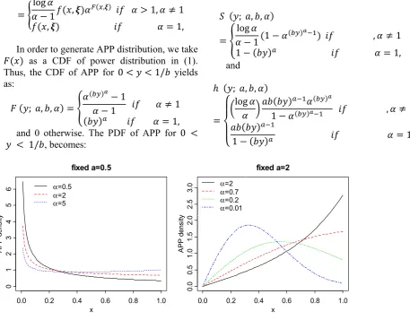
In order to generate APP distribution, we take
( ) as a CDF of power distribution in (1). Thus, the CDF of APP for 0 < < 1/ yields as:
( ; , , ) =
( ) − 1
− 1 ≠ 1 ( ) = 1,
and 0 otherwise. The PDF of APP for 0 < < 1/ , becomes:
( ; , , )
= log
− 1 ( ) ( ) , ≠ 1 ( ) = 1,
and 0 otherwise. We denoted the random variable that follows APP distribution by ∼
( , , ), where > 0 and > 0 are the shape parameters and > 0 is the scale parameter.
Results
Plots of the APP
Plots of the APP density function for selected choices of the parameters , and fixed scale parameter = 1 are given in Figure 1. The PDF of the APP distribution can be either unimodal or right skewed. If ≤ 1 and 0 <
≤ 1, then it is a decreasing function of , and for 0 < < 1 and > 1, it is an unimodal function.
The survival function, ( ), and the HRF,
ℎ( ), for APP distribution, are in the following forms for 0 < < 1/
( ; , , )
= log
− 1(1 − ( ) ) , ≠ 1 1 − ( ) = 1,
and
ℎ ( ; , , )
=
log ( ) ( )
1 − ( ) , ≠ 1
( )
1 − ( ) = 1,
Figure 1. Density plots of the APP distribution with various shape parameters and fixed scale parameter = 1.
0.0 0.2 0.4 0.6 0.8 1.0
01
2
3
4
5
6
fixed a=0.5
x
A
P
P
dens
ity
α=0.5
α=2
α=5
0.0 0.2 0.4 0.6 0.8 1.0
0.
0
0.
5
1.
0
1.
5
2.
0
2.
5
3.
0
fixed a=2
x
A
P
P
dens
ity
α=2
α=0.7
α=0.2
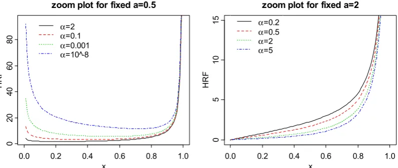
Plots of the HRF for selected choices of the parameters , and fixed scale parameter = 1 are given in Figure 2. If 1, then
ℎ ( ; , , ) is an increasing function of , and
ℎ ( ; , , ) can be a bathtub shaped for < 1, as tends to 0. The failure rate function is an important quantity characterizing life phenomena. Almost all of the standard distributions in statistics do not exhibit a bathtub shape for hazard rate function. Even the traditional Weibull distribution does not exhibit a bathtub shape for hazard rate function. Thus, it is important that one knows which distributions exhibit this shape and most real-life systems exhibit bathtub shapes for their hazard rate functions.
Mean residual lifetime function
The mean residual lifetime (MRL) function of APP distribution is given by
( ) = ( − | > )
= 1
( − ( ) ) (1 − )
− ( ) 1 − ( ) ! ( 1) .
For 0 < < 1 the MLR function can be written as
( )
=
1, − log − 1, −( ) log − (1 − )
( ( ) − ) ,
where ( , ) = is the
incomplete gamma function. If 1, then the APP distribution has increasing hazard rate function and hence, decreasing MRL function. For < 1 and close to 0, the APP distribution has bathtub-shape hazard rate function and hence, upside-down bathtub-shape MRL function.
Mode, quantile and simulation
The Mode of APP distribution can be obtained using the following simple formula:
=1 1 − log .
The − ℎ quantile of APP distribution is given by
=1 log ( − 1) 1
log . (2)
The median can be derive from (2) by considering = 0.5 as
=1 log( 1) − log 2
log .
One of the advantages of the APP distribution is that its CDF has a closed form which helps us to generate random variables by using the following simple formula
=1 log ( − 1) 1
log ,
where is a uniformly distributed random variable on (0, 1).
Figure 2. The HRF of APP distribution with various shape parameters and fixed scale parameter = 1.
0.0 0.2 0.4 0.6 0.8 1.0
0
204
0
608
0
zoom plot for fixed a=0.5
x
HR
F
α=2 α=0.1 α=0.001 α=10^-8
0.0 0.2 0.4 0.6 0.8 1.0
0
5
10
15
zoom plot for fixed a=2
x
HR
F
132
Moments and moment generating function Let a random variable follows
( , , ). We derive infinite expansions for the -th ordinary moment of as
= ( )
= ( − 1) (log )
! ( ). (3)
If 0 < < 1 then (3) can be expressed with a simpler formula as
= ( ) = 1, − log
(1 − ) (− log ) .
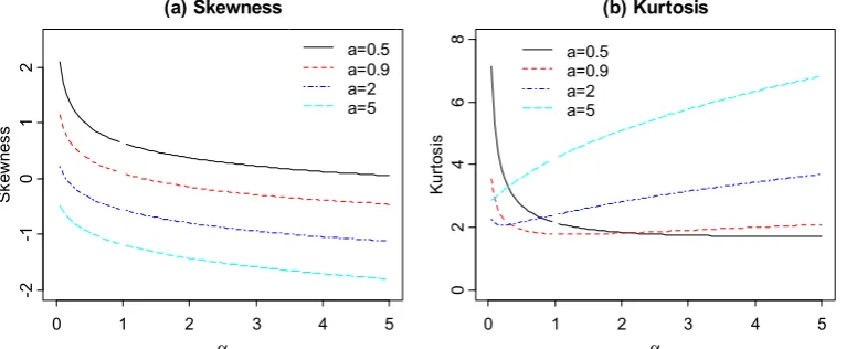
Based on the first four ordinary moments of the APP distribution, the measures of skewness
( ) and kurtosis ( ) of the APP distribution can obtained as
= − 3 2 ( − ) ,
and
= − 4 6 − 3 ( − ) .
Figures 3 (a) and (b) show the skewness and kurtosis of APP distribution as a function of parameter for different values of and fixed scale parameter = 1. It is observed that the skewness is a decreasing function of and kurtosis first decrease as increase and then start increasing.
The moment generating function (MGF) can be obtained by the following series expansion
( ) = ( ) ! .
So, the MGF of APP distribution is given by
( ) = − 1
(log )
! ( ).
Also, if 0 < < 1 then the MGF can be obtained using the following formula:
( )
= 1
− 1
1, − log
! (− log ) .
Order statistics
Order statistics make their appearance in many areas of statistical theory and practice. We now give the PDF of the -th order statistic =
: in a random sample of size from the APP distribution as follows
( ) = !
( − 1)! ( − )! ( ) 1
− ( ) ( )
= ! log ( − 1) ( )
(−1) ( )( )
( − − 1)! ( − − )! ! !
Entropies
Entropy has been used in various situations in Science and Engineering. The entropy of a random variable with PDF ( ) is a measure of variation of the uncertainty. There exist many entropy definitions and they are not equally good for all applications. While the most famous (and most liberal) Shannon (6) Entropy, which quantifies the encoding length, is extremely useful in information theory. Shannon showed important applications of this entropy in communication theory and many applications have been used in different areas such as Engineering, Physics, Biology and Economics. The Shannon entropy for APP distribution is obtained as
Figure 3. The skewness and kurtosis of APP distribution as a function of for some values of and fixed = 1.
0 1 2 3 4 5
-2
-1
0
1
2
(a) Skewness
α
S
kew
nes
s
a=0.5 a=0.9 a=2 a=5
0 1 2 3 4 5
024
68
(b) Kurtosis
α
Ku
rt
os
is
(− log ( )) = − log ∑ (log )
− 1 ( 1)( 1)!
( − 1) log ( 1)!
− log
! ( 2 ) . (4)
A generalized definition of entropy that stems from modifying the additivity postulate and results in a class of information measures that contain Shannons definitions as special cases is Rényi (7) entropy. If has the PDF f(x) then Rényi entropy is defined by
( ) = 1
1 − log ( )
where > 0 and ≠ 1. Using (4), the integral in ( ) for the APP distribution can be reduced to
( )
= log − 1
( log )
! ( − 1).
So, one obtains the Rényi entropy as
( )
= 1
1 − log
log − 1
log ( log )
! ( − 1) .
Discussion
Maximum likelihood estimation
We now determine the MLEs of the parameters of the APP distribution from complete samples only. Let , , . . . , be a sample from ( , , ) distribution. Then, the log-likelihood function is
log = log log log log − 1
( − 1) log
log .
The first order derivatives of log are
log
= log log
log log
log ,
log
= log ,
and
log
= − 1 − log
( − 1) log .
The MLEs of the unknown parameters cannot be obtained explicitly. They have to be obtained by solving some numerical methods, like Newton-Raphson or Gauss Newton methods or their variants. In this paper we use the optim function from the statistical software R (R Core Team, (8)) to maximize the logarithm of the likelihood function. This Fisher information matrix is important because it can be used to construct asymptotic confidence intervals for the parameters from its estimates. Let = ( , , ) and = ( , , ) denote the vector of parameters and its respective estimates. Under regularity conditions, the asymptotic distribution of is given by
√ − ~ 0, ( ) ,
where (θ) is expected information matrix. This asymptotic behavior is valid if (θ) is replaced by (θ) where (θ) is the observed information matrix evaluated at . The asymptotic multivariate normal 0, ( )
distribution can be used to construct approximate confidence intervals for the individual parameters and for the hazard rate and survival functions. Package numDeriv of R language can
134
be used to compute the Hessian matrix and its inverse, standard errors and asymptotic confidence intervals.
Application: glass fibres data
The following 46 data points represent the strengths of 15 cm glass fibres, originally obtained by workers at the UK National Physical Laboratory. The data set is obtained from Smith and Naylor (9). The sorted data are given as follows: 0.37 0.40 0.70 0.75 0.80 0.81 0.83 0.86 0.92 0.92 0.94 0.95 0.98 1.03 1.06 1.06 1.08 1.09 1.10 1.10 1.13 1.14 1.15 1.17 1.20 1.20 1.21 1.22 1.25 1.28 1.28 1.29 1.29 1.30 1.35 1.35 1.37 1.37 1.38 1.40 1.40 1.42 1.43 1.51 1.53 1.61.
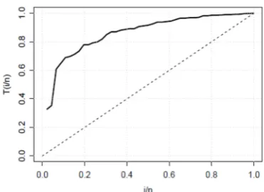
In order to identify the shape of the hazard function, we shall consider a graphical method based on the Total Time on Test (TTT) plot. In its empirical version the TTT plot is given by
( / ) =∑ :∑ ( − ) :
:
where = 1, 2, , and : represents the -th order statistic of the sample. If the empirical
TTT transform is convex, concave, first convex then concave, and first concave then convex, the shape of the corresponding hazard rate function is, respectively, decreasing, increasing, bathtub, and unimodal. (For more details, see Aarset, (10)). Figure 4 shows the empirical TTT plots for the glass fibres data, which is concave indicating an increasing failure rate function, which can be properly accommodated by APP distribution. We compare APP distribution with power distribution, BP distribution and Transmuted Power Function distribution (T-Ps) introduced by ul Haq et al.
11) with PDF
( ) = 1 − 2 ,
0 < < , > 0, > 0, −1 < < 1.
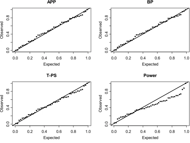
To see which one of these models is more appropriate to fit data. The MLEs of parameters, Akaike Information Criterion (AIC) value, Bayesian Information Criterion (BIC) value, Kolmogorov-Smirnov (K-S) statistic and its p-value are given in Table 1. The APP distribution
Figure 5. Probability plots for the fitted distributions
Table 1. The maximum likelihood estimates, AIC, BIC and K-S and its p-values for glass fibers data.
The model MLEs of the parameters AIC BIC K-S
statistic
p-value
APP = 4.6523, = 0.6211, = 0.0455 10.1961 15.68202 0.0699 0.9872 BP = 3.5953, = 0.5996, = 1.17, = 2.6908 12.7105 20.0251 0.0701 0.9770
T-Ps = 3.6454, = 1.61, = 0.8614 11.0284 16.5143 0.0895 0.8548
Power = 2.5565, = 0.6211 17.4726 21.1299 0.1963 0.0578
APP
Expected
Ob
se
rv
ed
0.0 0.2 0.4 0.6 0.8 1.0
0.
0
0.
4
0.
8
BP
Expected
Ob
se
rv
ed
0.0 0.2 0.4 0.6 0.8 1.0
0.
0
0.
4
0.
8
T-PS
Expected
Ob
se
rv
ed
0.0 0.2 0.4 0.6 0.8 1.0
0.
0
0.
4
0.
8
Power
Expected
Ob
se
rv
ed
0.0 0.2 0.4 0.6 0.8 1.0
0.
0
0.
4
0.
gives the smallest AIC, BIC and K-S statistics. The probability plots for the fitted distributions are plotted in Figure 5. It is clear from Table 1 and Figure 4 that the APP model provides the best fits to the data.
Conclusion
In this paper, we proposed a new family of distributions called alpha-power power distribution (APP), by applying the alpha-power transformation method initially proposed by Mahdavi and Kundu (5) to the classical power distribution. The HRF of the APP distribution can be a bathtub shape that is important quantity characterizing life phenomena. Various properties of the new distribution are obtained. These properties include moments, quantiles, mode, moment generating function, order statistics and some entropies. We dis-cuss maximum likelihood estimation of the model parameters and derive the observed information matrix. An application of the APP distribution is demonstrated in a real data set. It provides a better fit than other competing models.
Conflicts of interests
The authors declare that there is no conflict of interest regarding the publication of this article.
References
1. Boyce JK, Klemer AR, Templet PH, Willis CE. Power distribution, the environment, and public health: A state-level analysis. Ecologic Econom. 1999;29(1):127–140.
2. Van Dorp JR, Kotz S. The standard two-sided power distribution and its properties: with applications in financial engineering. Am Stat. 2002;56(2):90–99.
3. Cordeiro GM, dos Santos Brito R. The beta power distribution. Braz J Probabil Stat. 2012; 26(1):88–112.
4. Balakrishnan N, Nevzorov V. A primer on statistical distributions. Hoboken, New Jersey: A John Wiley & Sons; 2003.
5. Mahdavi A, Kundu D. A new method for generating distributions with an application to exponential distribution. Commun Stat Theory Method. 2017;46(13):6543–6557.
6. Shannon CE. Prediction and entropy of printed English. Bell System Technic J. 1951;30(1):50– 64.
7. Rényi A. On measures of entropy and information. In Proceedings of the Fourth Berkeley Symposium on Mathematical Statistics and Probability, Volume 1: Contributions to the Theory of Statistics. The Regents of the University of California; 1961.
8. R Core, Team R. A Language and Environment for Statistical Computing. R Foundation for Statistical Computing, Vienna, Austria; 2017. 9. Smith RL, Naylor JA. Comparison of maximum
likelihood and bayesian estimators for the three-parameter weibull distribution. Appl Stat. 1987; 358–369.
10. Aarset MV. How to identify a bathtub hazard rate. IEEE Transact Reliabil. 1987;36(1):106– 108.