Journal of Computing and Security
Expected Coverage of Perfect Chains in the Hellman Time Memory
Trade-Off
Nasser Hossein Gharavi
a,∗, Abodorasoul Mirghadri
a, Mohammad Abdollahi Azgomi
b,
Sayyed Ahmad Mousavi
caFaculty of Communication and Information Technology, Imam Hossein University (IHU), Tehran, Iran. bIran University of Science and Technology (IUST), Iran.
cShahid Bahonar University of Kerman, Kerman, Iran.
A R T I C L E I N F O.
Article history:
Received:18 January 2017
Revised:16 September 2017
Accepted:16 November 2017
Published Online:10 February 2018
Keywords:
Time Memory Trade-Off, Perfect Chains, Random Mapping, Expected Value.
A B S T R A C T
Critical overlap situations in the classical Hellman’s cryptanalytic time memory trade-off method can be avoided, provided that during the precomputation phase, we generate perfect chains which are merge-free and loop-free chains. In this paper, we present asymptotic behavior of perfect chains in terms of time memory trade-off attacks. More precisely, we obtained expected values and variances for the coverage of perfect chains. We have also confirmed our theoretic outcomes with test results.
c
2016 JComSec. All rights reserved.
1
Introduction
Cryptanalytic time memory trade-offs (TMTO) have been introduced in 1980 by Hellman [1]. He tried to find an optimal solution between two extremes in searching of the large search spaces: the time-consuming exhaustive searching and the memory-consuming lookup tables. In its more general form, TMTO can be viewed as a general one-way function inverter. Let X be a search space of sizeN andf :
X → X be a one-way function,i.e., a function which
is straightforward to compute, but which will be hard to invert. An example of interest is the— the function mapping a secret key to the encryption of a specific fixed known plaintext. TMTO is universal (indepen-dent of the type of functionf) method for searching the solutions of the equation f(x) = y, for a fixed imagey∈ X.
∗ Corresponding author.
Email addresses:[email protected](N.H. Gharavi),
[email protected](A. Mirghadri),[email protected](M. Abdollahi Azgomi),[email protected](S.A. Mousavi)
ISSN: 2322-4460 c2016 JComSec. All rights reserved.
In precomputation phase (offline phase) of the Hell-man’s method, we generatemchains oft+ 1 points from the search spaceX following a simple rule that in each chain, image of preceding point under the func-tionf is the next point. In the attack phase (online phase), these chains can be used for searching the solu-tions of the equationf(x) =y, for a given image point
y∈ X. This is accomplished by determining a specific chain that possibly includesy and searching through this chain. Consequently, the number of chains (m), as well as their lengths (t) are mostly selected in such a way that the number of points inside chains is ap-proximately equal toN (the search space size).
success of the attack.
Two basic improvements of the Hellman’s method, that we are not treating in this work, are Distinguished Points (DP) method, which is attributed to Rivest in [2] and Rainbow method [3], announced by Oechslin; for more details regarding these methods see [4,5].
For constructing an efficient TMTO table, we must confirm that the usage of our memory is certainly effi-cient. Consequently, in the precomputation phase, we should avoid storing repeated part of the chains, which merged with previously recorded chains or looped with itself. In DP and Rainbow methods, generally, more chains than really required are produced and then chains with similar ending points are removed. The resulting tables are calledperfect tables[4–8]. In fact, perfect tables are tables in which merges and loops are occurred rarely.
Unlike DP and Rainbow methods, the removal of redundancies in classical Hellman’s method cannot be done easily. In this paper, we will consider a generic procedure, introduced in the papers [6,8], for con-structing perfect version of the Hellman tables in pere-computation phase. During this technique, whenever a loop within a chain is found, construction of the chain might be terminated. Also, when a chain is merged with a previously constructed chain, the redundant part of the later chain will be omitted. This procedure guarantees unique elements in the table,i.e., it leads us to perfect chains.
The main disadvantage of this approach, is that ev-ery single element of each chain that is created must looked up in all of the previously produced chains. The authors of the paper [8] offered to track the record of points previously included within the chains through-out the offline phase. On the other hand, these look ups can be performed efficiently using some high-speed cycle detection and merge detection algorithms [9–11].
In the perfect type of the TMTO techniques, char-acteristics of chains (for example the average lengths, coverage, and variances) shed more light on the per-fect chain creation procedure, as well as, make it pos-sible for getting a much better understanding of the TMTO. The performances of the perfect version of the DP and Rainbow methods are completely analyzed earlier and we are really not planning to discuss about them; for example you can see [4,5,12]. Additionally, there are several analysis for perfect chains behavior in the classical Hellman’s method [6,8], however at this point there isn’t any explicit expression for the expected values and variances of the coverage of per-fect chains in the classical Hellman’s method. In this paper, we are going to obtain asymptotic formulas for expected values, and variances of the coverage of
perfect chains in classical Hellman’s method. In the next section (Section2), the basic Hellman time memory trade-off, its limitations and the per-fect version of this method are described. In the Sec-tion 3, an asymptotic probabilistic analysis of the perfect chains is presented. More explicitly, expected values and variances for the coverage of perfect chains are obtained. Section 4is devoted to experimental results of our theoretical formulas. We show experi-mentally that the theoretical results match practical outcomes. Finally, Section5provides a short summary and overview of the future works on this problem.
In the last of this section, note that, nevertheless in TMTO procedures we make use of a particular one-way functionf, we can assume that f is a random mapping. This assumption is done by any theoretic analysis of trade-off algorithms. In very rough terms, a random mapping f : X → X is a function that assigns independent and random valuesf(x)∈ X to each of its argumentsx∈ X [13,14].
2
Hellman’s Method and Its Perfect
Version
In the Hellman’s TMTO method, starting from a random pointx0∈ X, iteratively evaluatingf, a chain
of lengthtis generated as follows:
x0 f
→x1=f(x0) f
→x2=f2(x0) f
→ · · ·→f xt=ft(x0).
Let positive integersmandtthat satisfy the relation
mt2≈N(matrix stopping rule) be fixed. To construct
aHellman matrixof sizem×(t+1), pickingmrandom start points, chains of lengtht are created. In order to save memory, just the first and last columns of the Hellman matrix are kept in a table, known asHellman table. Additionally, the table is sorted with respect to end points for speeding up the lookups in attack phase; for more details see [1,4,5].
SP1=x10 x11 x12 x13
. . .
x1(t−1) x1t=EP1SP2=x20 x21 x22 x23
. . .
x2(t−1) x2t=EP2SP3=x30 x31 x32 x33
. . .
x3(t−1) x3t=EP3...
...
SPm=xm0 xm1 xm2 xm3
. . .
xm(t−1) xmt=EPmf f f f f f
f f f f f f
f f f f f f
f f f f f f
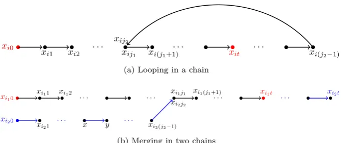
In the Hellman’s method, one will try to be able to keep as many different points as possible by generating as long chains as possible; but various critical overlap scenarios can appear and increase constraints of the method.
(2) Two chains can merge. This is the case where there exist i1 6=i2such that xi1j1 =xi2j2, for
some j1 and j2. Which means that from the
moment of the merge until the end of at least one chain, both chains include exactly the same points (Figure1(b)).
Consequently, multiple occurrences of points lead to a lower coverage ofX. Coverage of a Hellman matrix is defined as the number of distinct entries in this matrix, or the number of elements in the set H =
Sm
i=1
St−1
j=0f
j(x
i0).
In the paper [1], lower and upper bound for the expected coverage of a Hellman matrix is obtained as follows
m X
i=1
t−1
X
j=0
1− it
N
j+1
≤E[|H|]≤mt. (1)
One of the main consequences of overlap situations is thefalse alarmphenomena. Let image pointy∈ X
is given. There exist situations in which the chain that has been produced fromy, in the online phase, merges with some other chain that is saved in the Hellman table, which unfortunately does not includey(see the Figure1(b)). Therefore, looking for a matching end point does not essentially imply that the imagey will be found in the regenerated chain through the related start point. As illustrated in Figure 1(b), a wrong starting point xi10, instead ofxi20, will be searched
in the online phase andxcan’t be found.
In order to construct a perfect table version of the Hellman’s method, we will consider a generic proce-dure, introduced in the papers [6,8], for constructing perfect chains in perecomputation phase. LetSf(x) =
{ft(x) :t≥0}be the set of all distinct elements in the chain starting fromx∈ X. At this point we describe the procedure of generating perfect chains:
• Given a random point x10 ∈ X. We generate
the chain starting from x10 and we terminate
construction of the chain, when a loop appears. The event for the number of points in this chain is denoted by Ch1, or equivalently Ch1=|Sf(x10)|.
• Fori≥2, a random pointxi0∈ X is chosen and
we generate the chain starting fromxi0. When
the chain merged with a previously constructed chain or when a loop occured, we stop the process. The event for the number of elements ini’th chain is denoted by Chi. Note that
Chi=
Sf(xi0)/
i−1
[
j=1
Sf(xj0)
fori≥2.
We follow this constructionmtimes as follows which results in mperfect chains, where Chj =ij forj =
1,2, . . . , m.
SP1=x10 x11 x12
. . . .
x1i1=EP1SP2=x20 x21 x22
. . . .
x2i2=EP2SP3=x30 x31 x32
. . . .
x3i3=EP3...
...
SPm=xm0 xm1 xm2
. . .
xmim=EPmf f f f
f f f f
f f f f
f f f f
As you observe, this method ends up with a number of chains with variable lengths, where all elements in chains are distinct.
The main disadvantage of this procedure, which make it probably impractical, is that every single ele-ment of every chain that is produced, has to be looked up in all formerly generated chains. For this reason, Avoine et al. [6] stated that constructing perfect Hell-man tables is not efficient. In [8], the authors suggest to keep the record of points already included in to chains efficiently by using interval trees in the precom-putation phase. However these look ups increase the precomputation complexity, the actual profits of the method which relies on perfect chains depends both on the implementation of look ups and characteristics of the chains. On the other hand, in the online phase of this approach there is no false alarm and it is possi-ble to have a high probability of success. By the way, using most efficient cycle detection and collision detec-tion algorithms [9–11] in the precomputation phase, we can decrease the precomputation complexity.
In the next section, we present a probabilistic analy-sis of the perfect chains characteristics. More precisely, we are interested in the expected values and variances of the random variables Chi, and
Ci = Ch1+· · ·+Chi = i [
j=1
Sf(xj,0), for 1≤i≤m.
Note that, the random variable Chi indicates the
coverage ofi’th perfect chain and the random variable
Ci indicates the coverageiperfect chains.
· · · · xi0
xi1 xi2 xij1
xij2
xi(j1+1) xit xi(j2−1)
(a) Looping in a chain
· · · ·
· · · ·
xi10
xi11 xi12 xi1j1 xi2j2
xi1(j1+1) xi1t xi2t
xi20
xi21 x y xi2(j2−1)
(b) Merging in two chains
Figure 1. Merging and Looping in Chains
3
Analysis of the Perfect Chains
In this section, we are going to discuss about expected values of the random variables ChiandCifor 1≤i≤ m. Since we supposed thatf is a random mapping, we can assume that we have an urn containing N
distinctly marked balls and these balls are drawn from the urn, one at a time, with replacements. Indeed, the random variable Ch1counts the number of balls that
must be drawn in order to obtain a repeated value. So we have
Pr[Ch1=k1] =
k1−1
Y
i=0
N−i N
!
k1 N
Pr[Ch2=k2|Ch1=k1] =
k2−1
Y
i=k1 N−i
N
!
k1+k2 N
Pr[Ch2=k2|Ch1=k1,Ch2=k2] =
k3−1
Y
i=k1+k2
N−i N
!
k1+k2+k3 N
.. .
Pr[Chm=km|Ch1=k1, . . . ,Chm−1=km−1] =
km−1
Y
i=k1+···+km−1
N−i N
k1+· · ·+km N
By multiplying above conditional probabilities, we have
Pr[Cm=k] =
X
k1+···+km=k
k1≥1,k2,...,km≥0
Pr[Ch1=k1, . . . ,Chm=km]
=
k−1
Y
i=0
N−i N
!
k
NmPm−1(k),
where,
Pm−1(k) =
X
k1+···+km=k
k1≥1,k2,...,km≥0
k1(k1+k2)· · ·(k1+· · ·+km−1).
Letl1=k1, l2=k1+k2, . . . , lm−1=k1+· · ·+km−1.
Then 1≤l1 ≤l2 ≤ · · · ≤lm−1 ≤k and we obtain
that
Pm−1(k) = k X
lm−1=0
lm−1
lm−1
X
lm−2=0
lm−1· · ·l2 l2 X
l1=0
l1.
SoPm(k) =P k
x=0xPm−1(x), which satisfy in
assump-tions of the Lemma2.
Since asiN, NN−i ≈e−i/N [4, Appendix A], the asymptotic expected value of the random variableCm,
asN tends to infinity, is as follows
E[Cm] =
N X
k=0
kPr[Cm=k]
= 1
Nm N X
k=0
k−1
Y
i=0
N−i N
!
k2Pm−1(k)
≈
iN
1
Nm N X
k=0
k2Pm−1(k)e−
k2 2N ≈ N→∞ N Nm Z 1 0
(N x)2Pm−1(N x)e−
N
2x 2
dx.
Let Pm−1(x) = P 2m−2
j=0 am−1,jxj. Therefore as N → ∞we obtain that
E[Cm]≈
1
Nm−3
Z 1
0 x2
2m−2
X
j=0
am−1,j(N x)j e −N 2x 2 dx =
2m−2 X
j=0
am−1,j Nj Nm−3
Z 1
0
xj+2e−N2x 2
dx
.
So by using Lemmas 2and3 we easily conclude that,
E[Cm]≈
(2m−1)! (2m−1(m−1)!)2
r
πN
ex-pected value of the coverage ofmperfect chains, as
N tends to infinity.
Similar to above procedure and by using Lemmas2 and3we derive
E[Cm2] =
N X
k=0
k2Pr[Cm=k]
≈
2m−2 X
j=0
am−1,j Nj Nm−4
Z 1
0
xj+3e−N2x 2
dx
≈2mN+O(√N).
Thus, the asymptotic value for the variance of the coverage ofmperfect chains is obtained as follows, as
N tends to infinity.
V[Cm] =E[Cm2]−(E[Cm])2
≈
2m−
π
2
(2m−1)! (2m−1(m−1)!)2
!2
N+O(
√
N).
(3) Now, sinceE[Chm] =E[Cm]−E[Cm−1], we easily
conclude that, asN tends to infinity
E[Chm]≈
2m(2m−1)! (2m(m)!)2
r
πN
2 +O(1). (4)
Note that by using Equation (4),E[Ch1]≈ q
πN
2 .
This result has been investigated previously in the standard birthday problem for a year with N days; for example see [15,16] and the brilliant paper [13].
Evidently, asm→ ∞, by using the Sterling formula,
m!≈mme−m√2πm, and the Equations (2) and (4)
we have
E[Cm]≈
p
2N(m−1), asm→ ∞, (5)
E[Chm]≈
s
N
2(m−1), asm→ ∞. (6) So we obtain that
E[Cm]E[Chm]≈N, asm→ ∞. (7)
The Equations (2), (4), (5), (6) and (7) indicates how one can choose parameters to obtain an efficient per-fect table. For example, when we want to have a full coverage of the search space, then the average number of the perfect chains is obtained as follows
E[Cm]≈
p
2N(m−1) =N ⇒m= N 2 + 1. Also, for m = N2 + 1, we have E[Chm] ≈ 1 is the
minimum chain length.
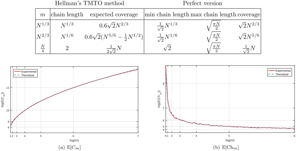
The perfect and non-perfect Hellman’s TMTO methods for different values ofm, with matrix
stop-ping rulemt2=N, are compared in the Table1.
4
Experimental Results
During this section, we provide some experiments which are carried out to check of our theoretic results made in the former section. The numerical results are calculated using the Matlab software.
In our tests, the random mappingf is constructed from the mini-AES (16-bit) cipher [17]. Our reasons for choosing this specific algorithm are: (1) The search space of mini-AES is small against AES algorithm and we can use this algorithm more times for testing our theoretical data; (2) almost all functions derived from mini-AES algorithm, using a constant plaintext, have properties of a random function [13].
More explicitly, the random mapping f : X → X maps the 16-bit key in X = {0,1}16 to 16-bit
ciphertext in X under a fixed plaintext. Different fixed plaintexts are used to create multiple random mappings. Also, starting pointsxi,0∈ X, 1≤i≤m,
are generated randomly. Then we explicitly computed Ch1=|Sf(x1,0)|, Chi=|Sf(xm,0)/∪ji−=11 Sf(xj,0)|, C1=|Sf(x1,0)|, Ci=∪ij=1Sf(xj,0),
for 2≤i ≤m, on the search space of sizeN = 216.
Finally, numerous test instances are conducted for different random starting points. The average values in our test instances are given in Figure2((a) and (b)). It can be seen that the experimental curve is nearly close to the theoretical curve, obtained by the Equations (2) and (4).
5
Summary and Conclusions
Within the basic Hellman’s TMTO approach, points are generated and immediately contained into the current chain until a fixed chain length is achieved, and after that we start the creation of the next chain. In the case of perfect Hellman’s TMTO approach, the current chain is finished if a previously employed point happens again. This method results in a number of chains with variable lengths where all points inside all chains are distinct and hence 100% coverage of the search space can be guaranteed. Such perfect chains would certainly ensure the discovering of the solutions of the equationf(x) =y, thus, making this technique deterministic.
or-Table 1. Comparison of the Perfect and Non-Perfect Hellman’s TMTO Methods, for Different Values OfmWithmt2=N.
Hellman’s TMTO method Perfect version
m chain length expected coverage min chain length max chain length coverage
N1/3 N1/3 0.6√2N2/3 √1
2N
1/3 qπN
2
√
2N2/3 N2/3 N1/6 0.6√2(N5/6−1
2N
1/2) √1
2N
1/6 qπN
2
√
2N5/6 N
4 2
1
2√2N
√
2 qπN
2
1 √
2N
1 2 3 4 5 6 7
log(m) 8
9 10 11
log(E(C
m
))
Experimental Theoretical
(a)E[Cm]
0 1 2 3 4 5 6
log(m) 4
5 6 7 8
log(E(Ch
m
))
Experimental Theoretical
(b)E[Chm]
Figure 2. Theoretically and Experimentally Obtained E[Cm] And E[Chm], for 1≤m≤27 And N = 216 (With mini-AES
Algorithm).
der to obtain these characteristics, we used an asymp-totic probabilistic analytical model, which treats the chain generation as a random process.
Although, for large search spaces, loop and collision detection algorithms for generating perfect chains in the precomputation phase may not be practically feasible, our analysis provides a deeper understanding of the statistical details of the perfect chains.
References
[1] Martin Hellman. A cryptanalytic time-memory trade-off.IEEE transactions on Information The-ory, 26(4):401–406, 1980.
[2] Dorothy Elizabeth Robling Denning. Cryptogra-phy and data security. Addison-Wesley Longman Publishing Co., Inc., 1982.
[3] Philippe Oechslin. Making a Faster Cryptanalytic Time-Memory Trade-Off. InCrypto, volume 2729, pages 617–630. Springer, 2003.
[4] Jin Hong and Sunghwan Moon. A comparison of cryptanalytic tradeoff algorithms. Journal of cryptology, 26(4):559–637, 2013.
[5] Ga Won Lee and Jin Hong. Comparison of perfect table cryptanalytic tradeoff algorithms. Designs, Codes and Cryptography, 80(3):473–523, 2016. [6] Gildas Avoine, Pascal Junod, and Philippe
Oech-slin. Characterization and improvement of time-memory trade-off based on perfect tables. ACM Transactions on Information and System Security
(TISSEC), 11(4):17, 2008.
[7] Johan Borst, Bart Preneel, and Joos Vandewalle. On the time-memory tradeoff between exhaustive key search and table precomputation. In Sym-posium on Information Theory in the Benelux, pages 111–118. TECHNISCHE UNIVERSITEIT DELFT, 1998.
[8] Violeta Tomaˇsevi´c and Milo Tomaˇsevi´c. An anal-ysis of chain characteristics in the cryptanalytic TMTO method. Theoretical Computer Science, 501:52–61, 2013.
[9] Antoine Joux. Algorithmic cryptanalysis. CRC Press, 2009.
[10] Gabriel Nivasch. Cycle detection using a stack.
Information Processing Letters, 90(3):135–140, 2004.
[11] Paul C Van Oorschot and Michael J Wiener. Par-allel collision search with cryptanalytic applica-tions. Journal of cryptology, 12(1):1–28, 1999. [12] Jin Hong. Perfect Rainbow Tradeoff with
Check-points Revisited. PloS one, 11(11):e0166404, 2016.
[13] Philippe Flajolet and Andrew M Odlyzko. Ran-dom mapping statistics. In Workshop on the Theory and Application of of Cryptographic Tech-niques, pages 329–354. Springer, 1989.
[14] Valentin Fedorovich Kolchin. Random graphs, volume 53. Cambridge University Press, 1999. [15] Bernard Harris et al. Probability distributions
Mathematical Statistics, 31(4):1045–1062, 1960. [16] Herman Rubin and Rosedith Sitgreaves.
Prob-ability distributions related to random transfor-mations of a finite set. Technical report, Stan-ford Univ Ca Applied Mathematics and Statistics Labs, 1954.
[17] Raphael Chung-Wei Phan. Mini advanced encryp-tion standard (mini-AES): a testbed for crypt-analysis students. Cryptologia, 26(4):283–306, 2002.
[18] John H Conway and Richard Guy. The book of numbers. Springer Science & Business Media, 2012.
A
Some Lemmas
The following lemmas are used in this work.
Lemma 1 (Faulhaber’s formula [18]). Let P(x) =
Px
k=1k
p= 1p+ 2p+· · ·+xp. ThenP(x)is a
polyno-mial of degreep+ 1with the fillowing form
P(x) = 1
p+ 1
p X
i=0
(−1)i
p+ 1
i
Bixp+1−i,
whereBi =Pik=0Pkv=0(−1)v vkv m
k+1, fori= 0,1, . . .,
are the Bernoulli numbers.
Lemma 2. LetPm(x) = Pj2m=0am,jxj be a
polyno-mial of degree2msuch that
Pm(x) =
x−1
X
i=m
iPm−1(i), P0(x) = 1, m≥1.
Then
am,2m=
1 2mm!.
Proof. Let Pm(x) = P
2m
j=0am,jxj. So Pm−1(x) =
P2m−2
j=0 am−1,jxj and
Pm(k) =
k−1
X
x=m
xPm−1(x) =
k−1
X
x=m
x
2m−2
X
j=0
am−1,jxj
=
2m−2 X
j=0
am−1,j
k−1
X
x=m
xj+1
!
=
2m−2 X
j=0
am−1,j
k−1
X
x=0
xj+1−
m−1
X
x=0
xj+1
!
.
Therefore by using the Lemma1we have
Pm(k) = 2m−2
X
j=0
am−1,j
1
j+ 2k
j+2+O(kj+1)
= am−1,2m−2
2m k
2m+O(k2m−1).
So, we obtain that
am,2m=
am−1,2m−2
2m , a0,0= 1, a1,2=
1 2.
(A.1) Solving the recursive relation (A.1) is easy and
am,2m=
1
2×4× · · · ×2m =
1 2mm!.
Lemma 3. LetIj = R1
0 e
−N
2x 2
xjdxforj ≥0. Then
asN→ ∞we have the following asymptotic formulas
I2j≈
(2j)!
j!2jNj r
π
2N, I2j+1≈ j!2j Nj+1.
Proof. First note that
I0=
Z 1
0 e−N2x
2
dx=
r 2π N Z √ N 0 1 √
2πe −1 2y 2 ≈ N→∞ r π 2N and
I1=
Z 1
0 e−N2x
2
xdx= 1
N
1−e−N2
.
Let du = e−N2x 2
xdx and v = xj−1 for j ≥ 2. We
obtain that
Ij=−
1
Ne −N
2 +j−1
N Ij−2, j≥2.
AsNtends to infinityIj≈ j−N1Ij−2and so by solving
this recursive relation we have
I2j ≈
1×3×5× · · · ×(2j−1)
Nj I0≈
(2j)!
j!2jNj r
π
2N, I2j+1≈
2×4×6× · · · ×(2j)
Nj+1 I1≈
Naser Hossein Gharavireceived his B.Sc. in Telecommunication Engineering from Uni-versity of Tehran, M.Sc. degree in Cryptogra-phy from Imam Hossein University and Ph.D. degree in Cyber Defense Engineering from Imam Hossein University, Tehran, Iran, in 1996, 2002 and 2017, respectively. His research interests include cryptography, cryptanalysis, security protocols and network security.
Abdolrasoul Mirghadrireceived his B.Sc., M.Sc. and Ph.D. degrees in Mathematical Statistics, from the Faculty of Science, Shiraz University in 1986, 1989 and 2001, respec-tively. He is an associate professor at the fac-ulty and research center of communication and information technology, Imam Hussein University, Tehran, Iran since 1989. His re-search interest includes: Cryptography, Statistics and Stochas-tic Processes. He is a member of ISC scientific society.
Mohammad Abdollahi Azgomireceived his B.Sc., M.Sc. and Ph.D. degrees in com-puter engineering (software) (1991, 1996 and 2005, respectively) from Department of Com-puter Engineering, Sharif University of Tech-nology, Tehran, Iran. His research interests include modeling and evaluation of security, privacy and trust, network security, and soft-ware security. He is currently an associate professor at School of Computer Engineering, Iran University of Science and Tech-nology, Tehran, Iran.