Journal of Computing and Security
An Efficient End to End Key Establishment Protocol for Wireless
Sensor Networks
Ali Fanian
a,∗
Mehdi Berenjkoub
aaDepartment of Electrical and Computer Engineering, Isfahan University of Technology (IUT), Isfahan, Iran.
A R T I C L E I N F O.
Article history:
Received:05 November 2012
Revised:06 April 2013
Accepted:28 June 2013
Published Online:20 December 2013
Keywords:
Wireless Sensor Networks, Key Management, Network Security, Random Key Pre-distribution, Symmetric Polynomial, Deployment Knowledge, Combinatorial Design.
A B S T R A C T
Sensor networks are eligible candidates for military and scientific applications such as border security and environmental monitoring. They are usually deployed in unattended or hostile environments; therefore, security is a major concern with these networks. A fundamental requirement is the capability to establish pairwise keys between sensors. Many key establishment protocols have been proposed to address the security issues in wireless sensor networks. However, most of these protocols have security and/or performance restriction. In this article, we propose a new key establishment protocol based on symmetric polynomials and random key pre-distribution. In our protocol, contrary to others, we use several symmetric polynomials to generate polynomial shares for a group of sensors, and the distribution of polynomial shares to each sensor is done using a combinatorial design. Since a limited number of shares are generated from a symmetric polynomial, the polynomial degree is very low. As a result, the common key between sensors can be generated without imposing significant overhead to them. Further, in the proposed protocol, key establishment between near sensors is provided via symmetric polynomials, while key establishment between far sensors is accomplished via random key pre-distribution. Using these two techniques simultaneously allows end to end key establishment between every pair of sensors with reasonable overhead.
c
2014 JComSec. All rights reserved.
1
Introduction
Due to the technological achievements in recent decades, wireless networks are now widely deployed and highly developed. According to the application, there are many types of wireless networks, including sensor networks. Sensor networks are usually con-structed from a large number of limited resource
∗ Corresponding author.
Email addresses:[email protected](A. Fanian),
[email protected](M. Berenjkoub)
ISSN: 2322-4460 c2014 JComSec. All rights reserved.
critical aspect of network security. In the literature, key management protocols are based on either sym-metric or asymsym-metric encryption techniques. Due to resource limitations in the sensors, protocols based on asymmetric cryptography are not suitable [6,7]. To date, many different methods have been proposed for key management in sensor networks [8–16]. Some of these distribute sensors in the network uniformly [8– 11] so sensors can reside at any point in the network with equal probability. Key establishment with these methods presents both security and performance challenges. Others have tried to improve performance using node deployment knowledge. This knowledge is used in the pre-deployment stage to arrange the sensors into groups [12–16]. Some of the proposed pro-tocols are based on random key pre-distribution. In these schemes, one key may be used for several pairs of sensors, so perfect security cannot be achieved. With perfect security, the security between two un-compromised sensors must be guaranteed despite other sensors being compromised. Some protocols are based on threshold cryptography. While perfect security can be achieved with this technique, the memory usage and processing overhead are very high. Further, in most of the proposed protocols, end to end key establishment between every pair of sensors creates significant communication overhead. In this article, an efficient end to end key establishment pro-tocol (ETE) is proposed which uses both symmetric polynomial and random key pre-distribution methods. This improves the security, and also the scalability so that the sensor overhead due to the protocol is not excessive. A preliminary version of this article was presented in [17], however in this article the proposed key establishment for near and far sensors are consid-ered simultaneously. Also the technical correctness of the proposed protocol is precisely evaluated.
The features of the proposed protocol are as follows:
• The polynomial shares are distributed in groups based on combinatorial design theory.
• Shared keys between sensors within each group are directly established based on their polynomial share derived from a symmetric polynomial.
• Keys between two sensors which are not in the same group but are near to each other are in-directly generated by intermediate nodes called agents. Keys are sent from the source sensor to the destination sensor via a secure path generated by agent sensors.
• Key establishment between far sensors is provided by random key pre-distribution.
• End to end key establishment between every pair of sensors in the network can be achieved without significant overhead.
• The proposed protocol can provide connectivity
and resistance against key exposure for a large network with relatively low resource consump-tion.
• Perfect security can be supported in the proposed protocol.
• The proposed protocol is more efficient in terms of processing overhead than other schemes. The rest of the article is organized as follows. Sec-tion2reviews some required primitives including re-lated work. Details of our key establishment protocol are given in Section3. Performance evaluation and se-curity analysis of the proposed protocol are presented in Section4. Finally, some conclusions are given in Section5.
2
Preliminaries
In this section, we present authentication using sym-metric polynomials and review related results in the area.
2.1 Authentication Using Symmetric Polyno-mials
A symmetric polynomial [11], [18, 19] is a t-degree (K+ 1)-variate polynomial defined as follows
f(x1, x2, . . . , xk+1) =
t
X
i1=1
t
X
i2=1
· · ·
t
X
ik+1=1
ai1,i2,...,ik,ik+1x
i1xi2. . . xikxik+1
(1) All coefficients of the polynomial are chosen from a finite fieldFq, whereqis a prime integer. The poly-nomialf is a symmetric polynomial in the following sense [11]
f(x1, x2, . . . , xk+1) =f(x∂(1), x∂(2), . . . , x∂(k+1))
(2) This means that for any permutation,∂, we obtain the same polynomial. Every node using the protocol based on a symmetric polynomial takes identities (I1, I2, , IK) from the key management center, and stores these in memory. The key management center must also compute a polynomial share for each node using its identities and the symmetric polynomial. The coefficientsbiK+1 stored in node memory as the share
of the polynomial coefficients are obtained using the following expression
f(u(x) =f(I1, I2, . . . , Ik, x) = t
X
iK+1=1 biK+1x
iK+1
identities of nodesuandvhave one mismatch in their identities given by (c1, c2, . . . , ci−1, ui, ci+1, . . . , cK) and (c1, c2, . . . , ci−1, vi, ci+1, , cK), respectively. In or-der to compute a common key, nodeutakesvi as the input and computesfu(vi), and nodevtakesuias the input and computesfv(ui). Due to polynomial sym-metry, both nodes compute the same key. In [11], it was shown that in order to maintain perfect security in the sensor network, the polynomial degree must satisfy the presented inequalities in4and5.
0≤Ni−1≤t (4)
Ni×
K+1
r
K(K+ 1)!
2 ≤t (5)
whereNiis the number of nodes in groupiandi= 1,2, . . . , K
2.2 Combinatorial Design Theory
Combinatorial design theory is the study of arranging elements of a finite set into patterns such as subsets or arrays according to specified rules. For instance, one such design is a Balanced Incomplete Block Design (BIBD). ABIBD is an arrangement of a finite set
S ofvdistinct object into a collectionBofbblocks such that every block has k distinct objects. Each object occurs inrdifferent blocks, and each pair of
S certainly occurs in λ blocks. The design can be expressed as (v, b, r, k, λ) whereλ(v−1) =r(k−1) andbk=vr[20,21]. ABIBDis called a symmetric
BIBD when b = v and r = k. In this case, each block has k=robjects and each object is inr=k
blocks. For example consider a (v,b,r,k,λ) = (7, 7, 3, 3, 1) symmetric design. LetS ={1,2,3, . . . ,7}, so the setShas 7 objects, and there are 7 blocks. Each block has 3 objects, and each object occurs in 3 blocks. Every pair of distinct objects occurs in only one block. Consequently, every pair of blocks intersects in only one object. Using a construction algorithm, the blocks are:{1,2,3},{1,4,5},{1,6,7},{2,4,6},{2,5,7},{3,4,7},
{3,5,6}. A subset of symmetricBIBDsis called Finite Projective Planes. These planes consist of a finite set
P points and a set of subsets ofP, called lines. For an integerq, (q2), the finite projective plane has four properties: 1) every line contains q+1 points; 2) every point occurs in q+ 1 lines; 3) there are q2+q+ 1 points as objects; 4) there are q2+q+ 1 lines as
blocks. Therefore, a finite projective plane of order
qis a symmetric design with parameters (q2+q+ 1,
q2+q+ 1,q+ 1,q+ 1, 1) [20,21].
2.3 Related Work
Due to resource constraints in the sensors, key man-agement is not a trivial task in WSNs. Thus, many
key establishment protocols have been proposed to address the security issue in WSNs. Eschenauer et al. [8] proposed a random key pre-distribution scheme. Before sensor deployment, keys from a large key-pool are selected randomly and stored in the sensors. Af-ter deployment, with some probability they can es-tablish a key between each other. If there is no com-mon key between two sensors, a comcom-mon key can be generated through an intermediate node which has common keys with both. Zhou et al. [11] proposed a key management protocol based on symmetric poly-nomials. In this scheme, at-degree (K+ 1)-variate symmetric polynomial is selected and each sensor has aK-tuple of identities. Then the polynomial share for each sensor is computed using these identities and the symmetric polynomial. The polynomial share and sen-sor identities are stored in the sensen-sor. If the identities of two sensors differ in only one dimension, they can produce a common key. Liu et al. proposed another key management protocol based on symmetric poly-nomials [10]. In their approach, a grid based model is used to calculate and distribute the sensor polynomial shares. TheN sensors in the network form anm×m
matrix (N =m2). For each row and column of this
matrix a t-degree bi-variate symmetric polynomial is selected. A sensor in position (i, j) of the matrix computes polynomial sharesfc
j(x, j) andfir(i, y) from symmetric polynomialsfc
j(x, j) andfir(i, y), respec-tively. Therefore, if two sensors are in the same row or column, they can compute a common key directly. Otherwise, they have to employ another sensor to com-pute this key. Note that the sensor deployment model in this method does not follow any distribution, so the sensors are distributed randomly in the network. Some WSN key management schemes use deploy-ment knowledge to improve the protocol performance. In [13], [15] it was shown that if deployment knowl-edge is used before the sensors are deployed, the ef-ficiency of the protocol can be increased. Du et al. [13] proposed a key management protocol based on the approach in [8] which uses deployment knowledge during key distribution. This knowledge is modeled us-ing a Gaussian probability distribution function (pdf). Conversely, methods which do not use deployment knowledge follow a uniform model, so the sensors can reside at any point in the network with equal proba-bility. In [13] the network area is divided into square cells and each cell is considered the location for one group of sensors. Then the key-pool is divided into sub key-pools (equal to the number of cells) such that each sub key-pool has some key correlation with its neighboring sub key-pools. Each sensor in a cell has
se-lected from a smaller key-pool. This can improve the protocol performance, especially in large networks.
Lin et al. [12] proposed a key management protocol called LPBK in which the network area is divided into square cells. Each cell has a specific symmetric poly-nomial which is used to compute a polypoly-nomial share for the sensors in the corresponding cell and the four adjacent vertical and horizontal cells. In this scheme, each sensor stores five polynomial shares in its mem-ory. Zhou et al. [14] proposed a key management pro-tocol called LAKE which is based on symmetric poly-nomials and deployment knowledge. Similar to the previous scheme, the network is divided into square cells and each sensor is allocated to a cell. The polyno-mial in this method is at-degree tri-variate symmetric polynomial. Each sensor in this protocol has a pair of identities (n1, n2) wheren1represents the cell
iden-tity andn2represents the sensor identity within the
cell. Each sensor receives a polynomial share based on its identities. After network deployment, sensors with just one mismatch in their identities can directly compute a common key.
Yu et al. [16] proposed another key management protocol based on an approach by Blom [22]. Blom developed a protocol that allows each pair of nodes to establish a common key. With this scheme, if no more thantnodes are compromised, all common keys of the uncompromised nodes remain secure. A (t+ 1)×N
matrixGis defined as public information whereN
is the size of the network. During the key generation phase for the sensor nodes, the key management server creates a secure random (t+ 1)×(t+ 1) symmetric matrix,D. Then the server calculates anN×(t+ 1) matrixA = (D×G)T, whereT denotes transpose. SinceDis symmetric,K=A×Gis also symmetric, so thatKij =Kji. In Bloms scheme,Kij is used as a common key between nodesiandj. Hence, nodesiand
jshould be able to computeKijandKji, respectively. Nodeistores theith row ofAand theith column of
G. Hence, if nodesiandjwant to establish a common key, they should exchange their columns ofGand then computeKij =Kjiusing their private row ofA. In the Yu et al. scheme, the network area is divided into hexagonal cells and the information from theGandD
matrices is stored in the sensors based on deployment knowledge. A secret matrixAi(equivalent to matrixD in the Blom method), is allocated to celli. The sensors in the cell are each assigned a row fromAi. Hence, the sensors belonging to a cell can produce a common key directly. To generate a common key between sensors belonging to different cells, another secret matrix,
B, is used that is common to sensors in neighboring cells. These matrices are allocated to the cells using two parametersb andw. Parameterb indicates the number ofB matrices assigned to a group, andwis
the number of rows chosen by a sensor. The analysis in [16] shows that the best results are obtained with
w=2 andb=2. In this method, the cells are divided into two categories, base cells and normal cells. Base cells are not neighbors to each other, but every normal cell is a neighbor of two base cells and four normal cells. To produce a common key between sensors in neighboring cells, a confidential matrixBis allocated to each base cell together with its six neighbors. Bloms scheme is used with this matrix to provide information to the sensors. Therefore, the sensors in the seven neighboring cells can produce a common key directly. Since every normal cell is neighbor with two base cells, their sensors receive information from twoBmatrices. Although this scheme has connectivity near to one, the memory consumption is extremely high. Du et al. [15] proposed another key management protocol using Blom scheme. In this scheme, many pairs of matrices
G andD, called the key space, are produced, and some key spaces are assigned to each cell. Adjacent cells have some common key space as in [13], where adjacent cells have correlation between their sub key pools. Each sensor selects key spaces randomly, and according to Blom scheme, the required information is stored in the sensors. As a result, sensors with the same key space can produce a common key. As in [13], two vertical or horizontal neighboring cells have common key spaces, and two diagonal neighboring cells have common key spaces, where is the number of key spaces assigned to a cell.
In [23], a hybrid key establishment protocol for low resource wireless sensor networks based on Blom scheme and random key pre-distribution was pro-posed. In this protocol, the network area is divided into non-overlapping hexagonal cells, and key estab-lishment between sensors in a cell is provided by Blom scheme. Key establishment between sensors residing in neighboring cells is provided via pre-distributed random keys.
More-over, if the number of sensors belonging to a group increases, in perfect security conditions the computa-tion overhead become considerable.
3
The End to End Key Establishment
Protocol (ETE)
We propose a new key management protocol called ETE. Both symmetric polynomials and random key pre-distribution are used to improve efficiency. Simi-lar to other schemes [12–15], key information is dis-tributed to the sensors during the pre-deployment stage. Once the sensors have been deployed, they can produce a common key either directly or indirectly. Due to the use of two methods in ETE, two types of information must be stored in the sensors. One is the sensor polynomial shares generated using the symmet-ric polynomials and finite projective planes, while the other is a set of random keys.
There are two types of key generation in ETE. In the first type, a common key between near sensors is generated via their polynomial shares. In the second type, a common key between far sensors is generated using the pre-distributed random keys. Since in this case a key may be selected by several sensors, the common key between two far sensors may also be used by other pairs of sensors. Conversely, the common key between near sensors is unique. As we will show, end to end key establishment between every pair of sensors can be supported without significant overhead.
A common key between far sensors may be required in situations where environmental information is trans-mitted to servers far from the network area. Hence, the information must be relayed between sensors to reach the servers. Thus an authenticated route must be established between sensors or between sensors and servers by using a secure routing protocol such as Karlof [26], Ariaden [27] and endairA [28]. In a se-cure routing protocol, the intermediate sensors which establish the route must all be authenticated. This is necessary to prevent an adversary from deceiving the server with false information. In other words, if the intermediate sensors rely only on authenticated information from the other sensors, adversaries or ma-licious sensors cannot send false information through the network. To achieve this security, each sensor must be able to authenticate the other sensors. Therefore, the sensors should be able to establish a common key with every other sensor. Thus in the proposed proto-col, as in [13,14], a goal is the capability of generat-ing a key between every pair of sensors. With other schemes, intermediate nodes must be used to estab-lish a common key between far sensors [12], [16]. Be-cause the number of intermediate nodes may be large,
the possibility of common key exposure is high, and the use of these nodes increases the communication and computational overhead. Key generation between near sensors will, however, occur more frequently than between far sensors, so we use different key genera-tion processes for near and far sensors to achieve high performance. Moreover, in ETE, we use deployment knowledge to distribute key information among the sensors. ETE consists of three phases: key and polyno-mial share pre-distribution, direct key establishment and indirect key negotiation. We next introduce the models used in ETE, and then discuss the key man-agement phases in detail.
3.1 ETE Models
In this section we introduce both the security and network models used in ETE.
3.1.1 Deployment Model
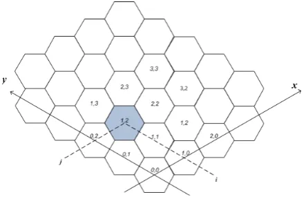
As shown in [13], [15] deployment knowledge can be used to improve network connectivity and increase key management performance. As mentioned before, the key management schemes based on deployment knowledge such as [13–16] use a Gaussian distribution for the distribution of sensors in the network. In ETE, the network area is divided into non-overlapping hexagonal cells, and the sensors are allocated in groups to these cells. The center of a cell is defined as the deployment point of the sensors allocated to that cell. Figure1shows the division of the network into hexagonal cells. Each cell in ETE has a pair of identities (i, j) which is the cell position. Using two-dimensional Cartesian coordinates and assuming that the deployment point of cellCi,j is (xi, yi), the pdf of the sensor resident points can be formulated as
fkij(x, y|kCi,j) =f(x−xi, y−yj) = 1
2πσ2e
−[(x−xi)2+(y−yi)2]/2σ2
where
f(x, y) = 1 2πσ2e
−[x2+y2]/2σ2 (6) Assuming the same pdf for all groups, we use
fk(x, y|kCi,j) instead of fkij(x, y|kCi,j). As shown in [15], the distance between the deployment point and resident point of a sensor is less than 3σ with probability 0.9987, whichσis the standard deviation. 3.1.2 Security Model
Figure 1. Deployment points for a two-dimensional sensor network
1- Generating the Polynomial Share based on Symmetric BIBD
In the key establishment protocols based on thresh-old cryptography such as Blom scheme or symmetric polynomials, some shares are generated from a secret for many sensors in a group. Hence, to achieve perfect security the threshold must be set very high. As we show in the processing analysis section, increasing the threshold causes a significant increase in processing overhead. Thus in the proposed protocol, contrary to other schemes, we use several symmetric polynomials instead of one, but each symmetric polynomial gener-ates a limited number of polynomial shares for sensors. In other words, each sensor in a group has several poly-nomial shares, but the polypoly-nomial degrees are very low. Increasing the number of symmetric polynomials for a group may create some difficulties in the key es-tablishment protocol. For example, some sensors may have more than one polynomial share from the same symmetric polynomial, or some sensors may have no shares from the same polynomial. Therefore in ETE, the distribution of polynomial shares is very critical to the protocol performance, so we use combinatorial de-sign theory to distribute polynomial shares in a group. As mentioned previously, a symmetric BIBD can be represented using the parameters (v,b, r, k, λ). Since in a symmetric BIBDv=bandr=k, we can represent it by (v, k, λ), where v is the number of distinct objects, k is the number of distinct object in a block and λ is the number of times a pair of objects occurs in the blocks. We use a symmetric BIBD for distributing symmetric polynomial shares to the sensors.
In the proposed protocol, a symmetric polynomial is as an object in the symmetric BIBD and each sensor is a block. A symmetric polynomial is used to generate a common key between two sensors, so the intersection of the assigned symmetric polynomials for two sensors should be one. As a result, we assume
λ=1. Thus, we consider a finite projective plane of
order q with parameters (q2+q+ 1, q+ 1,1), andq
should be chosen such thatq2+q+ 1 is greater than
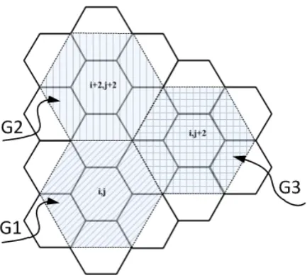
the number of sensors in a group,N g. As mentioned in Section3.1.1, the network area is partitioned into hexagonal cells, and the cells are divided into base cells and normal cells. Base cells are not neighbors, but normal cells are neighbors with two base cells and four other normal cells. Each normal cell is divided into two virtual regions. As shown in Figure2, a group consists of a base cell and virtual regions in the six neighboring cells. In this figure, cells (i, j), (i, j+ 2) and (i+ 2, j+ 2) are base cells and G1, G2 and G3 are groups and other cells are normal cell. The half of each normal cell is virtual region. Each virtual region belongs to one group, so q should be chosen according to this group size. To construct a symmetric design, we use (q−1) Mutually Orthogonal Latin Squares (MOLSs). A MOLS is aq×qarray such that each of theq symbols occurs exactly once in each row and column [20, 21]. For exampleL1 andL2 below are
two MOLS of order 3.
L1=
1 3 2 2 1 3 3 2 1
L2=
1 3 2 3 2 1 2 1 3
According to [20, 21], a symmetric BIBD with (q2, q,1) is called affine plan. Thereforeq2 blocks of an affine plane can be constructed using the generated MOLS and then the blocks of the projective plane can be constructed from this affine plane. The blocks of the finite projective plane fromL1 andL2 are the
following.
A1 = (1,1),(2,2),(3,3),(4,1)
A2 = (1,3),(2,1),(3,2),(4,1)
A3 = (1,2),(2,3),(3,1),(4,1)
A4 = (1,1),(2,3),(3,2),(4,2)
A5 = (1,3),(2,2),(3,1),(4,2)
A6 = (1,2),(2,1),(3,3),(4,2)
A7 = (1,1),(1,2),(1,3),(4,3)
A8 = (2,1),(2,2),(2,3),(4,3)
A9 = (3,1),(3,2),(3,3),(4,3)
A10= (1,1),(2,1),(3,1),(4,4)
A11= (1,2),(2,2),(3,2),(4,4)
A12= (1,3),(2,3),(3,3),(4,4)
Now we have 13 blocks that represent the sym-metric block design. Note that the symsym-metric design conditions are satisfied by these blocks, and it has parameters (q2+q+ 1, q+ 1,1). In our protocol, we use the finite projective plane to distribute polyno-mial shares to sensors in a group. As mentioned pre-viously, the groups of sensor are constructed and a finite projective plane is used for a group. Since ob-jects are symmetric polynomials and blocks are sensor nodes, we must generateq2+q+ 1≥4N
csymmetric polynomials for each group, whereNcis the number of sensors in a cell. Each symmetric polynomial is a
t-degree bi-variate symmetric polynomial, given by
f(x1, x2) =Pti1=1Pti2=1ai1,i2x
i1
1x
i2
2. Each sensor in
ETE has three identities (i, j, k). The first two identi-ties (i, j) are the deployment point of the sensor and the last identitie (k) is the unique sensor identity in the cell. Based on the finite projective plane, q+ 1 symmetric polynomials are assigned to a sensor. For each symmetric polynomial, the sensor polynomial sharebvi2 is generated as follows
fkv(x) =fi,jv = t
X
i1=1
t
X
i2=1 ai1,i2x
i1
1x
i2
2 b
v i2
t
X
i1=1 ai1,i2k
i1
wherev{1,2, . . . , q2+q+ 1}.
Since every pair of sensors in a group have a poly-nomial share from the same symmetric polypoly-nomial, they can directly establish a common key. However, sensors belonging to different groups cannot establish a common key directly or even indirectly. This cre-ates isolated components within the network. Thus in the proposed protocol, we use another finite projec-tive plane for each normal cell. As shown in Figure2, half of the sensors belonging to a normal cell are in one group, and the others belong to a second group. Hence, two sensors in a normal cell that belong to different groups cannot establish common key. Using the new finite projective plane, we want to generate polynomial shares for sensors that belong to a normal cell. This requires the generation ofq2+q+ 1≥N
c symmetric polynomials similar to those for the first finite projective plane. Thenq+ 1 polynomial shares are computed and assigned to each sensor.
2- Random Key Selection
In methods based on random key pre-distribution, some keys are selected randomly from a key-pool with size S and assigned to the sensors. As mentioned in Section2.2, in [13] the global key-pool is divided into sub key-pools and each sub key-pool is assigned to a cell so that neighboring cells have some correlation in their sub key-pools. By correlation we mean that the intersection of the two sets is nonzero. Since random keys are only used for far sensors in ETE, contrary to [13], neighboring cells should not have any correlation
Figure 2. The group model in the proposed protocol
in their sub key-pools. Thus, sensors in base cells should select their random keys from separate sub key pools. In other words, in the proposed protocol, sensors in a normal cell receive two sets of polynomial shares from two finite projective planes, but the sensors in base cells receive only one set of polynomial shares from one projective plane. Hence, the memory used in base cell sensors is less than that used in normal cell sensors, so we only assign random keys to sensors in base cells.
According to the proposed model, the global key pool is divided intoNc sub key-pools and each sub key-pool has S/Nc keys, and each sensor in a base cell selects keys from a specific sub key pool based on its identity, so all sensors in base cells with the same identity select random keys from the same sub key pool. This ensures that two sensors in the same cell do not select keys from the same sub key pool. In addition, the sub key-pool assigned to a given sensor can easily be determined. This greatly simplifies key discovery, as will be described later.
3.2 Key Establishment by Near Nodes
and a common key will be established using the pre-distributed random keys. Due to the distribution of random keys in ETE, the logical distance between two cells using the same sub key-pool is three. Therefore,
dT lshould be less than this distance, so two sensors are said to be near if their logical distance is less than three. Key establishment between sensors falls into three categories as described below.
3.2.1 Direct Key Generation
Sensors belonging to the same cell can produce a common key directly. Since the real distance between them may be greater than the wireless transmission range, intermediate sensors may be required to relay the information. Some sensors located in neighboring cells may belong to the same group. They can also produce a common key directly. In fact, some sensors in all six normal cells adjacent to a base cell will have suitable polynomial shares. Note that the number of sensors belonging to a group is 4×Nc. According to the model in Section3.1.2, two sensors can easily determine if they are in the same group. If they belong to the same group, they can produce a common key by exchanging their unique identities as shown below
f1(k2) =
t
X
j=0
bj1k2j=K1−2
, f2(k1) =
t
X
j=0
bj2k1j=K2−1 (7)
3.2.2 Indirect Key Generation between Two Sensors
Sensors belonging to two distinct cells may reside adjacent to each other. If they cannot establish a common key directly, a proper agent node must be used. A proper agent is a node that has common keys with both of them. For example, in Figure2, suppose that node u from cell C(i,j) belonging to group G1 wants to establish a common key with node v from cell (i+1,j+2) belonging to G2. First, node u must find two agent sensors in cell (i+1,j+1), one belonging to G1 and another belonging to G2. Then nodeugenerates
Kuvas a common key and sends it to the agent nodes via a secure channel. The agent nodes receive this key and send it to v via a secure channel. Note that there are Nc/2 candidates for each agent node, where Nc is the number of sensors in a cell. If the deployment distance of two sensors belonging to two cells is more than 3 cells, random key pre-distribution is used for indirect key generation. Otherwise, since these sensors have not any polynomial share from similar symmetric polynomial, they have to use some agent nodes to establish common key. Therefore, in this situation,
the key establishment imposes significant overhead to sensor nodes. Note that if the distance between the resident points of the agents is less than the wireless transmission range, they will communicate with each other directly. Otherwise, a routing protocol can be used between them as in [8–15].
3.3 Key Generation between Far Sensors
If two sensors are far from each other, generating a common key using agents and their polynomial shares can be time consuming, and creates a security risk if nodes have been compromised. In this case, instead of establishing a long path of agents, ETE uses the pre-distributed random keys stored in base cell sensors. As mentioned previously, all sensors in a base cell have some random keys selected from separate sub key-pools. If two sensors select their random keys from the same sub key-pool, they can establish a common key. Otherwise, another sensor must be used. Due to the proposed random key pre-distribution, sensors with the same identity belonging to different base cells have selected keys from the same sub key-pool. Hence, there areNcsensors in each cell which can be used as an agent sensor to establish a common key between two sensors that reside in far cells. If two sensors belonging to normal cells want to establish a common key, they must select two sensors from base cells with the same identity as agent nodes. Therefore, the number of agents required is two. If there is no common key between these sensors, another pair of sensors in the base cells must be selected to reinitiate the process of key establishment. This is repeated until a common key is established between agents in the two cells.
4
Security Analysis and Performance
Evaluation
In this section the security analysis and performance evaluation of the proposed protocol are presented and compared with similar protocols. Based on the discus-sion in Section2.2, the best candidates for compar-ison with ETE are LPBK [12], LAKE [14], and the protocols by Yu et al. [16] and Du et al. [15].
4.1 Network Configuration
The network parameters are as follows:
• The number of sensors in the network is N = 10000
• The network area is 1000×1000m2
• The sensor locations have a two dimensional Gaus-sian distribution with standard deviation
• The number of sensors deployed in each cell is 100 4.2 Determining the Polynomial Degree
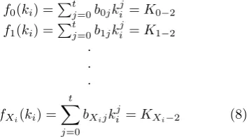
To satisfy the perfect security condition, the security between two uncompromised sensors must be guaran-teed despite the existence of compromised sensors. As mentioned in Section3.2, in ETE direct key genera-tion via a symmetric polynomial is limited toq+ 1 sensors. Thus in this case, if an adversary wants to obtain the common key between two sensors, it must compromise a number of sensors who have polynomial shares generated from the same polynomial. This re-quires that an adversary produce the polynomial share of either sensor. To do this, an adversary must solve an equation with (t+ 1) unknowns, i.e., the sensor polynomial share coefficientsbi2. By compromising Xisensors in the same group as sensori, an adversary can produce the following set of equations
f0(ki) =P
t
j=0b0jkij=K0−2
f1(ki) =Ptj=0b1jkij=K1−2
. . .
fXi(ki) =
t
X
j=0
bXijk
j
i =KXi−2 (8)
Since the polynomial share of the ith sensor has
t+ 1 coefficients, ifXiis less thant+ 1, an adversary cannot obtain this share. Therefore, if the number of sensors who have polynomial shares from a symmet-ric polynomial, Ni, is less than t+ 1, an adversary cannot compromise the common key between two un-compromised sensors, even if all other sensors are compromised.
For key management protocols based on symmet-ric polynomials and deployment knowledge, we must computeNi. In the proposed protocol, as shown in Figure2, each group includes all sensors belonging to a cell and some sensors in the six neighboring cells. However, in ETENiis equal toq+ 1 whereqsatisfies the conditionq2+q+ 1≥4Nc. With LPBK [12], the sensors in a cell along with its four horizontal and ver-tical neighbor cells have a polynomial share from the same symmetric polynomial. ThusNiis equal to 5Nc. In [14] each sensor has a polynomial share which can be used to directly produce a common key with all other sensors in its own cell andNc sensors in other cells. Therefore Ni is equal to 2Nc. To achieve full security with these methods, the polynomial degree must satisfy
Ni−2≤t (9)
In Table2, the required polynomial degree t is given for different protocols based on symmetric polynomials.
Table 1. The Minimum Polynomial Degree Required to Achieve Perfect Security
Protocol Polynomial Degree
LPBK [12] 498
LAKE [14] 198
ETE 19
4.3 Network Connectivity
Network connectivity is the ability to generate a com-mon key between sensors in the network. In [13], and [14] network connectivity is classified into two types: local connectivity and global connectivity. Local con-nectivity considers the probability of directly produc-ing a common key between adjacent sensors. Global connectivity is defined as the ratio of the number of nodes in the largest isolated component to the size of the network. For example, if the global connectiv-ity is 0.98, only two percent of the sensors cannot be accessed by the largest component. A network may have high local connectivity but there are some iso-lated components in the network. We define another type of connectivity called remote connectivity. Re-mote connectivity is the probability of producing a common key between far sensors. Note that if there is a common key between far sensors, intermediate sen-sors can act as routers so there is no need to establish a long key path.
4.3.1 Local Connectivity
Local connectivity is the probability of producing a common key between two adjacent sensors. Due to the polynomial share key generation mechanism in ETE, the probability of key generation between two adjacent sensors belonging to same group is one. However, some adjacent sensors do not belong to the same group, so they cannot establish a common key directly. To determine the local connectivity, we must determine the probability of producing common key for adjacent sensors. In [13,15] the probability of local connectivity is defined as
PL−C=p1/p2
p1=p(B(ni, nj)and A(ni, nj))
=X
jψ
X
iψ
P r(B(u, v)and A(u, v)|uCiand
vCj)×P r(uCi and vCj),
p2=
X
jψ
X
iψ
P r(A(u, v)|uCiand vCj)×
P r(uCiandvCj) (11) The interested reader is referred to [13,15] for de-tails. In this article, we use Equation11to compare the local connectivity with all methods. The value of
A(u, v) depends on the cell size, the number of sen-sors in each cell, the wireless transmission range, and the standard deviation of the Gaussian distribution for the sensors. These parameters are related to the network configuration introduced in Section4.1. With ETE, the probability of common key generation be-tween two sensors in cellsiandj, is given by
P(B(u, v)|uCi and vCj) =
1 ifi=j,
0.5 wherei, jdenotes a normal cell and its adjacent base cell, 0.25 wherei, jdenotes two adjacent
normal cells, 1− ScSc−r
/ Scr
where i, j denotes two base cells,
0 others
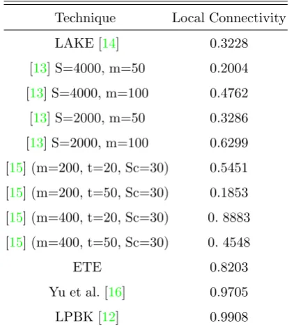
(12) whereScis the sub key pool size and r is the number of random keys selected by each sensor in a base cell. Local connectivity with the other methods was computed by considering the probability of generating a common key between sensors and Equation11. The results are shown in Table3. With the scheme in [13], each cell has a sub key-pool withSckeys. Some keys in a sub key-pool also exist in the sub key-pools of neighboring cells. In [13,15], it is assumed that each cell shares 15% of its keys with each horizontal and vertical neighboring cell sub key pool, and 10% with each diagonal neighboring cell sub key-pool. Thus each key in a sub key-pool may be selected by 2Ncsensors. Each sensor selects m random keys. Table 3shows that ETE has adequate connectivity, but the local connectivity with ETE is not as good as LPBK [12] and Yu [16]. However, as will be shown, considering memory usage, computational overhead and resilience against key exposure, ETE is much better than these schemes.
Table 2. The Local Connectivity of Different Techniques
Technique Local Connectivity
LAKE [14] 0.3228
[13] S=4000, m=50 0.2004 [13] S=4000, m=100 0.4762 [13] S=2000, m=50 0.3286 [13] S=2000, m=100 0.6299 [15] (m=200, t=20, Sc=30) 0.5451 [15] (m=200, t=50, Sc=30) 0.1853 [15] (m=400, t=20, Sc=30) 0. 8883 [15] (m=400, t=50, Sc=30) 0. 4548
ETE 0.8203
Yu et al. [16] 0.9705
LPBK [12] 0.9908
4.3.2 Remote Connectivity
Remote connectivity is the probability of directly producing a common key between two far sensors. This is crucial from the point of view of any two sensors securely communicating with each other in an efficient manner. As mentioned previously, pre-distributed random keys are used in ETE to establish a common key between far sensors, so we must analyze the probability of key generation in this situation. As described in Section3.2the global key pool is divided intoNcsub key-pools. In ETE, two far sensors with the same identity and belonging to different base cells selectrrandom keys from the same sub key-pool. The probability of establishing a common key in this case is
P r= 1−
Sc Sc−r
/
Sc r
Figure 3. Probability of establishing a common key between two far sensors with ETE
4.3.3 Global Connectivity
Global connectivity is the ratio of the number of nodes in the largest isolated component to the size of the entire network [13]. It is possible that a scheme has high local connectivity but many isolated network components. In this article we want to determine the affect of the key establishment protocol on global connectivity. We assume that every pair of sensors can directly or indirectly reach each other. In other words, we assume that the global connectivity disregarding key establishment is 100%. It is obvious that if the local connectivity is one, the global connectivity will be 100%. To determine the global connectivity, we have selected 1000 sensor nodes randomly and the percentages of sensors who can’t establish common key with any other sensors were computed. The results indicate that in the proposed protocol when the local connectivity is 0.50 and the remote connectivity is 0.36, only 0.0008 of the sensors are not accessible via a secure path. Thus global connectivity is not a concern. 4.4 Resilience against Node Compromising
Attack
Since the sensor hardware is not tamper proof, an adversary can capture the key material inside it [13]. By compromising some sensors, it may be possible to obtain the common key between uncompromised sensors. In this section, the effect of compromised nodes for both direct and indirect key generation is evaluated for ETE and the other methods.
4.4.1 The Probability of Direct Key Expo-sure
In methods based on symmetric polynomials, as shown in Section2.1, when an adversary compromises more than t sensors, they can access the common key be-tween uncompromised sensors. Therefore, in symmet-ric polynomial based methods, increasing t reduces the probability of revealing uncompromised keys (even to zero). However, a larger t means more processing and memory overhead for sensors, especially in large scale networks. Hence, t should be chosen based on the trade-off between memory and processing costs, and an acceptable security level. As mentioned in Sec-tion3.1.2, ETE restricts key generation with symmet-ric polynomials to sensors in the same group. If X is the number of compromised sensors in the network andNi is the number of sensors in each group, an adversary can obtain the common key between two un-compromised sensors if they can compromise at least t sensors in the group. The probability of this event is
Pc= Ni X
i=t+1
Ni
i
N−Ni
X−i
N X
(14)
This expression can be used to evaluate the resilience of ETE, LPBK and LAKE for the corresponding values of Ni, which were given in Section4.1. With ETE, due to the use of random keys for far sensors, we must also evaluate the effect of compromised sensors on the sensor resilience against random keys being revealed. As mentioned previously, the global key-pool is divided intoNc sub key-pools. Each sensor in a base cell is assigned to a sub key-pool and selects r random keys from it. Since each sensor in a base cell selects keys from a separate sub key-pool, the number of sensors which select the same sub key-pool isN/Nc . IfX sensors are compromised, the probability of compromising a sensor will beX/N, and the number of compromised sensors which select the same sub key-pool will be
X/Nc. Therefore, the probability of compromising a common key between two uncompromised far sensors is
Pc= 1−
1− r
S/Nc
NcX
(15) In [13], each sensor selects mR keys from a sub key pool. An adversary can get more information about the sub key pool by compromising more sensors. In this scheme, each cell has a sub key-pool withS keys, and each key exists in two neighboring sub key-pools. Thus, the probability of compromising the key between two sensors that have a common key is
1−1−mR
S
Xi
probability of compromisingXG sensors in a group whenXsensors are compromised in the entire network is
P(XG=i) =
X
i
(2
n)
i(1− 2
n)
X−i (17) wherenis the number of cells in the network. Therefore the probability of compromising a common key based on the pre-distributed random key approach in [13] is
PCom= 1−
min(2Nc,X) X
i=1
(1−mR
S ) i X i (2 n)
i(1−2
n)
X−i
(18) In [15], each sensor selects key spaces from available key spaces, and each key space is a Blom matrix. Sim-ilar to [13], each key space is shared between two neighboring cells and may be selected by 2Ncsensors. Whentsensors having distinct rows of the same key space are compromised, the other common keys in the key space are also compromised. Therefore, as-sumingXisensors in a group are compromised, the probability of compromising a common key between uncompromised sensors is
Xi X
i=t+1
X i i (τ Sc)
i(1− τ
Sc)
Xi−i (19)
Then the probability of compromising the common key between two uncompromised sensors whenX sensors are compromised in the entire network is
PCom= X
X
Xi
Xi X
i=t+1
X
Xi
(2
n)
Xi(1− 2
n)
X−Xi
X i i ( τ Sc)
i(1− τ
Sc)
Xi−i (20)
Based on Equations 14, 18 and20, the probability of direct key exposure between two uncompromised sensors is shown in Figure 4for different protocols. It can be seen that for near sensors, ETE provides greater resistance against direct key exposure than the other schemes. When the memory size is greater than 200, the security of LAKE is perfect. In Figure4, the memory size specifies the value of t for ETE, Du [13], Du [15], LPBK, and Yu [16]. Increasing the memory size will improve the security of these schemes based on Equation14. As shown in Figure4, the security of ETE is perfect when the memory size is greater than 400.
4.4.2 The Probability of Indirect Key Expo-sure
To produce a common key between two sensors not in the same group, agent sensors must be used. Therefore, if agents are compromised, an adversary can access common keys. In [8], it was shown that the average key
path length for two adjacent sensors is three sensors, while the length for far sensors is 11 sensors for a network similar to our configuration. The probability of revealing an indirect key,PRI, between two sensors
which usehsensors as agents is
PRI = 1−
N−h X
N X
(21)
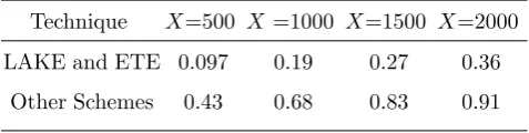
We simulated a sensor network with the configuration given in Section4.1. Our results indicated that with ETE, the average number of agents required for key establishment between far sensors is 1.9821. With LAKE, the corresponding number of agents is 1.3245. In Table4, the probability of indirect key exposure for different schemes is shown. In this table, the number of agents required for far sensors with LAKE and ETE is assumed to be two. The results in Table4 show that LAKE and ETE are much more resilient against indirect key exposure than the other schemes.
Table 3. Indirect Key Exposure Probability of Different Schemes
Technique X=500 X =1000 X=1500 X=2000 LAKE and ETE 0.097 0.19 0.27 0.36
Other Schemes 0.43 0.68 0.83 0.91
4.5 Memory Usage
In this section the memory usage of different schemes is calculated considering perfect security. To achieve perfect security when symmetric polynomials are used, the polynomial degree,t, must satisfy inequality 4. Blom scheme is at-secure scheme, so that if no more thantnodes are compromised, the link between un-compromised nodes will remain secure. In this case,t
(a) (b)
(c) (d)
Figure 4. Key resilience with different protocols for available memory (a) 250, (b) 350, (c) 450 and (d) 550.
Table 5. This shows that the memory required with LPBK and the approach in [16] is very large. The memory usage of the technique in [13] depends on the number of random keys (m). However, it cannot provide perfect security.
4.6 Computational Overhead
In sensors, a low power micro-controller is typically used as a processing unit, so we assume that an 8-bit micro-controller from the 8051 family is employed. To compare our proposed protocol with other schemes, we assume sufficient memory is available in the sensor. LPBK, LAKE and our proposed protocol are based on symmetric polynomials. If the polynomial has degree
t, 2tmodular multiplications and tsummations are required. We assume a key length of 128 bits. To compute the modular multiplication of two 128 bit numbers, we use the interleaved modulo multiplication
algorithm [29] which is implemented as follows Algorithm 1
Input: X, Y, M with 0≤X, Y ≤M
Output: P =X×Y modM n⇐number of bits inX xi⇐ithbit ofX
P⇐0
fori:=n−1toi≥0step−1do
P⇐2×P I⇐xi×Y
P⇐P+I
if P ≥M then
P⇐P−M
end if end for
multipli-Table 4. Memory Cost for Different Techniques
Technique Memory Cost Required Memory Cost for Direct Key Secrecy
LPBK[12] 5(t+ 1) 5(5Nc−2)
Du et al. [15] O(τ(t+ 1)) O(τ(t+ 1))
LAKE [14] t 2Nc−2
Yu et al. [16] 2(t+ 1) 2(7Nc−2)
ETE (q+ 1)t+r r+q2−1, q2+q+ 1≥4Nc,1≤r≤20
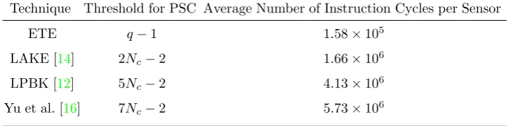
Table 5. Computational Overhead for Different Schemes
Technique Threshold for PSC Average Number of Instruction Cycles per Sensor
ETE q−1 1.58×10⁵
LAKE [14] 2Nc−2 1.66×10⁶
LPBK [12] 5Nc−2 4.13×10⁶
Yu et al. [16] 7Nc−2 5.73×10⁶
cation of two 128 bit numbers is approximately 4096 cycles. Hence, the number of instruction cycles is ap-proximately 8300tfor LPBK, LAKE and our proposed protocol. The value oftin these schemes is not iden-tical and is dependent on the group size. With the approach in [22], which uses Blom scheme for generat-ing common keys between sensors, multiplication of two matrices with dimensions (1, t+ 1) and (t+ 1,1) is required. For this operation,t+ 1 modular multipli-cations andt+ 1 summations are needed. Therefore, this scheme requires approximately 4096tinstruction cycles. These results are summarized in Table5for the Perfect Security Condition (PSC). This shows that our approach requires far fewer instruction cycles. Moreover, as shown in Figure3, because the proba-bility of the key establishment between far sensors in ETE, is close to one and the average number of agents required for key establishment between far sensors is 1.9821, as discussed in section4.4, ETE is more effi-cient than previous ones in terms of communication and computation overhead.
5
Conclusion
In this article, we introduced a new key management protocol called ETE which is based on symmetric polynomials and random key pre-distribution. Tradi-tional key establishment protocols based on symmet-ric polynomial use a polynomial to generate polyno-mial shares for a group of sensors. Due to the large number of sensors in a group, the required polynomial degree is quite high. This imposes a significant cost
in terms of memory usage and processing. In the pro-posed protocol, we use several symmetric polynomials for a group instead of one, and a combinatorial de-sign is used in the distribution of polynomial shares. Further, key establishment between near sensors is provided via symmetric polynomials, while for far sen-sors key establishment is accomplished via random key pre-distribution. Using both techniques, every pair of nodes can produce a common key either directly or in-directly. The simulation results indicate that the local connectivity with ETE is comparable to LPBK [12] and Yu [16], but the memory usage, computational overhead and resistance against key exposure is very efficient than these schemes. LAKE and ETE are only two schemes that can establish common key between far sensors. However, the local connectivity with ETE is more efficient than LAKE [14].
References
[1] Gregory J. Pottie and William J. Kaiser. Wireless integrated network sensors. Commun. ACM, 43 (5):51–58, 2000.
[2] Marcos A. Simpl´ıcio Jr., Paulo S. L. M. Barreto, Cintia B. Margi, and Tereza Cristina M. B. Car-valho. A survey on key management mechanisms for distributed wireless sensor networks.
Com-puter Networks, 54(15):2591–2612, 2010.
[3] Jennifer Yick, Biswanath Mukherjee, and Dipak Ghosal. Wireless sensor network survey.
Com-puter Networks, 52(12):2292–2330, 2008.
tracking using sensor networks. InWCNC, pages 1954–1961. IEEE, 2003. ISBN 0-7803-7700-1. [5] R.R. Brooks, P. Ramanathan, and A.M. Sayeed.
Distributed target classification and tracking in sensor networks. Proceedings of the IEEE, 91(8): 1163–1171, 2003. ISSN 0018-9219. doi: 10.1109/ JPROC.2003.814923.
[6] Ronald J. Watro, Derrick Kong, Sue fen Cuti, Charles Gardiner, Charles Lynn, and Peter Kruus. Tinypk: securing sensor networks with public key technology. In Sanjeev Setia and Vipin Swarup, editors,SASN, pages 59–64. ACM, 2004. ISBN 1-58113-972-1.
[7] David J. Malan, Matt Welsh, and Michael D. Smith. A public-key infrastructure for key dis-tribution in tinyos based on elliptic curve cryp-tography. InSECON, pages 71–80. IEEE, 2004. ISBN 0-7803-8796-1.
[8] Laurent Eschenauer and Virgil D. Gligor. A key-management scheme for distributed sensor networks. In Vijayalakshmi Atluri, editor,ACM Conference on Computer and Communications
Security, pages 41–47. ACM, 2002. ISBN
1-58113-612-9.
[9] Mi Wen, Yanfei Zheng, Wen jun Ye, Kefei Chen, and Weidong Qiu. A key management proto-col with robust continuity for sensor networks.
Computer Standards & Interfaces, 31(4):642–647, 2009.
[10] Donggang Liu, Peng Ning, and Rongfang Li. Es-tablishing pairwise keys in distributed sensor net-works.ACM Trans. Inf. Syst. Secur., 8(1):41–77, 2005.
[11] Yun Zhou and Yuguang Fang. A scalable key agreement scheme for large scale networks. In
Networking, Sensing and Control, 2006. ICNSC ’06. Proceedings of the 2006 IEEE International
Conference on, pages 631–636, 2006. doi: 10.
1109/ICNSC.2006.1673219.
[12] Donggang Liu and Peng Ning. Location-based pairwise key establishments for static sensor net-works. InIn 2003 ACM Workshop on Security
in Ad Hoc and Sensor Networks (SASN 03, pages
72–82. ACM Press, 2003.
[13] Wenliang Du, Jing Deng, Yunghsiang S. Han, Shigang Chen, and Pramod K. Varshney. A key management scheme for wireless sensor networks using deployment knowledge. In INFOCOM, 2004.
[14] Yun Zhou and Yuguang Fang. A two-layer key establishment scheme for wireless sensor net-works. IEEE Trans. Mob. Comput., 6(9):1009– 1020, 2007.
[15] Wenliang Du, Jing Deng, Yunghsiang S. Han, and Pramod K. Varshney. A key predistribution scheme for sensor networks using deployment
knowledge. IEEE Trans. Dependable Sec. Com-put., 3(1):62–77, 2006.
[16] Zhen Yu and Yong Guan. A key management scheme using deployment knowledge for wireless sensor networks. IEEE Trans. Parallel Distrib.
Syst., 19(10):1411–1425, 2008.
[17] A. Fanian and M. Berenjkoub. An efficient end to end key establishment protocol for wireless sensor networks. In Information Security and Cryptology (ISCISC), 2012 9th International ISC
Conference on, pages 73–79, 2012. doi: 10.1109/
ISCISC.2012.6408194.
[18] P Borwein and T Erd´elyi. Polynomials and
Poly-nomial Inequalities. Springer, New York, 1995.
[19] Yun Zhou and Yuguang Fang. Scalable link-layer key agreement in sensor networks. In Mil-itary Communications Conference, 2006.
MIL-COM 2006. IEEE, pages 1–6, 2006. doi: 10.1109/
MILCOM.2006.302079.
[20] Ian Anderson.Combinatorial designs and
config-urations. Ellis Horwood Chichester, 1990.
[21] Douglas R. Stinson.Combinatorial Designs:
Con-structions and Analysis. SpringerVerlag, 2004.
[22] Rolf Blom. An optimal class of symmetric key generation systems. In Thomas Beth, Norbert Cot, and Ingemar Ingemarsson, editors,
EURO-CRYPT, volume 209 ofLecture Notes in
Com-puter Science, pages 335–338. Springer, 1984.
ISBN 3-540-16076-0.
[23] Ali Fanian, Mehdi Berenjkoub, Hossein Saidi, and T. Aaron Gulliver. A new key establishment protocol for limited resource wireless sensor net-works. InCNSR, pages 138–145. IEEE Computer Society, 2010.
[24] T. Kavitha and D.Sridharan. Hybrid design of scalable key distribution for wireless sensor net-works. IACSIT International Journal of
Engi-neering and Technology, 2(2):136–141, 2010.
[25] Ali Fanian, Mehdi Berenjkoub, Hossein Saidi, and T. Aaron Gulliver. An efficient symmetric polynomial-based key establishment protocol for wireless sensor networks. ISeCure, The ISC In-ternational Journal of Information Security, 2(2): 89–105, 2010.
[26] Chris Karlof and David Wagner. Secure routing in wireless sensor networks: attacks and coun-termeasures. Ad Hoc Networks, 1(2-3):293–315, 2003.
[27] Yih-Chun Hu, Adrian Perrig, and David B. John-son. Ariadne: A secure on-demand routing pro-tocol for ad hoc networks. Wireless Networks, 11 (1-2):21–38, 2005.
[28] Gergely ´Acs, Levente Butty´an, and Istv´an Va-jda. Provably secure on-demand source routing in mobile ad hoc networks. IEEE Trans. Mob.
[29] Viktor Bunimov and Manfred Schimmler. Area and time efficient modular multiplication of large integers. InASAP, pages 400–. IEEE Computer Society, 2003. ISBN 0-7695-1992-X.
Ali Fanianreceived the Ph.D. degree from the Department of Electrical and Computer Engineering, Isfahan University of Technol-ogy in 2011. The title of his dissertation is Key Management Protocol in Wireless Sen-sor Networks. He started work in the same department as an Assistant Professor at that time. His research interests include ad-hoc networks, wireless network security and hard-ware design.

![Table 5. This shows that the memory required withLPBK and the approach in [16] is very large](https://thumb-us.123doks.com/thumbv2/123dok_us/41134.2004705/13.595.62.533.75.502/table-shows-memory-required-withlpbk-approach-large.webp)