University of Mazandaran, Iran
http://cjms.journals.umz.ac.ir
ISSN: 1735-0611
CJMS.4(1)(2015), 1-8
A Meshless Method for Numerical Solution of Fractional Differential Equations
Ahmad Golbabai 1Omid Nikan2
1,2 Department of Applied Mathematics, Iran University Science and Technology,P.O.Box,16844-13114,Narmak,Tehran,Iran.
Abstract.In this paper, a technique generally known as meshless numerical scheme for solving fractional differential equations is considered. We approximate the exact solu-tion by use of Radial Basis Funcsolu-tion (RBF) collocasolu-tion method. This technique plays an important role to reduce a fractional differential equation to a system of equations.The numerical results demonstrate the accuracy and ability of this method.
Keywords:Riemann-Liouville fractional integral,Caputo fractional derivative,Radial basis functions.
1. Introduction
The seeds of fractional calculus (that is, theory of integrals and derivatives of any arbitrary real or complex order) were planted over 300 years ago.Since then, many researchers have contributed to this field. Fractional calculus has gained considerable popularity and im-portance due to its attractive applications as a new modelling tool in a variety of scientific and engineering fields, such as viscoelasticity[1],hydrology[2], finance [3, 4], and system control[5]. In recent decades, the fractional calculus provides an excellent instrument for the description of memory and hereditary properties of various materials and processes. Furthermore, the fractional order models of real systems are regularly more adequate than usually used integer order models. Consequently, the field of the fractional differential equations has attracted interest of researchers in several areas including physics, chem-istry, engineering and even finance and social sciences. During the last decades, several
1[email protected] 2Corresponding author:omid
−[email protected] Received: 22 December 2013
Revised: 25 May 2014 Accepted: 22 July 2014
methods have been used to solve fractional differential equations. There are some further method, such as operational method,the Adomian decomposition method(ADM)[6], the homotopy perturbation method(HPM)[7, 10], the generalized differential transformation method(GDTM)[9]. In this work, we approximate the exact solution by use of Radial Basis Functions method(RBFs).We present the advantages of using the RBFs especially where in the data points are scattered. Radial basis function(RBF) is one of the most popular basis for construction of meshless methods. It is (conditionally) positive defi-nite, rotationally and translationally invariant.Over the last 27 years, RBF methods have become an important tool for the interpolation of scattered data and for solving partial differential equations[10].
RBF methods that use infinitely differentiable basis functions that contain a free parameter are theoretically spectrally accurate.The implementation of RBF methods involves solving a linear system that is extremely ill-conditioned when the parameters of the method are such that the best accuracy is theoretically realized. RBF methods that use infinitely differentiable basis.The existence of exact solution of fractional differential equation was discussed in Reference [5] and also the convergence of using this method was discussed in reference [11].
2. BASIC DEFINITIONS OF THE FRACTIONAL CALCULUS
In this section, we outline some preliminaries and notations, used throughout the re-maining sections of the paper[5].
Definition 2.1. A real function f(x), x >0 is said to be in the spaceCµ, µ∈Rif there exists a real number p(> µ), such that f(x) = xpf1(x) where f1(x) ∈ C[0,∞) and it is said to be in the spaceCµm iff f(m)∈Cµ, m∈N.
Definition 2.2. The Riemann-Liouville fractional integral of orderα of function f(x) ∈ Cµ, µ≥ −1 is defined as:
x
0Jαf(x) = Γ(α)1
∫x
0 (x−t)
α−1f(t)dt,
where Γ is the well-known Gamma function.
Lemma 2.3. Properties of the operator Jα can be found in [5], we mention only the following:
Forf ∈Cµ, µ≥ −1,
(1) JαJβf(x) =Jα+βf(x), f or all α, β≥0. (2) JαJβf(x) =JβJαf(x), f or all α, β ≥0. (3) Jαxγ = Γ(γ+α+1)Γ(γ+1) xγ+α α >0, γ >−1, x >0.
Definition 2.4. The Riemann-Liouville fractional derivative of orderαof functionf(x)∈ C−m1 is defined as:
x
0DαRLf(x) = dm dxm
(
1 Γ(m−α)
∫x
0 (x−t) m−α−1
f(t)dt
)
Definition 2.5. The fractional derivative off(x)∈C−m1 in the Caputo’s sense is defined as:
x
0DCαf(x) = 1 Γ(m−α)
∫ x
0
(x−t)m−α−1f(m)(t)dt, (2.1)
wherem=⌈α⌉.
The Caputo fractional derivative is considered because it allows traditional initial and boundary conditions to be included in the formulation of the problem.
Lemma 2.6. The defnitions above hold for functions f with special properties depending on the situations. It is clear that
(1) DβRL[D−RLαf(x)] =DRL−(α−β)f(x), ∀α, β≥0,
(2) x0DβRL[Jα] =Jα−β, ∀α, β≥0,
(3) DαRL[Jαf(x)] =f(x),
(4) Jα[x
0DαRLf(x)] =f(x)− ⌊∑α⌋
k=0 f(k)(0)
k! xk,
(5) x0DnRL [x0DRLα ] =x0DRLn+α, n∈N,
(6) x0DαC[x0DCn] =x0Dn+αC , n∈N,
(7) Jα[x0DαCf(x)] =f(x)− ⌊∑α⌋
k=0
f(k)(0+) k! xk,
(8) Jα[x0DαCf(x, t)] =f(x)− ⌊∑α⌋
k=0
∂k(x,0+)
∂tk xk k!,
(9) The fractional integral represents a convolution of power-law with a function f(x)
defined as:
(Jα f) (x) = tΓ(α)α−1 ∗f(x) = Γ(α)1 ∫0x(x−t)α−1f(t)dt.
Remark 2.7. We use the ceiling function ⌈α⌉ to denote the smallest integer greater than or equal to α, and the floor function⌊α⌋ to denote the largest integer less than or equal toα.
3. RBF INTERPOLATION
Franke also conjectured the unconditional nonsingularity of the interpolation matrix as-sociated with the MQ radial function,but it was not until a few years later, in 1986, that Charles Micchelli was able to prove it, making use of work by Schoenberg from the 30s and 40s.The main feature of the MQ method is that the interpolant is a linear combination of translations of a basis function which only depends on the Euclidean distance from its center. This basis function is therefore radially symmetric with respect to its center. The MQ method was generalized to other radial functions, such as the thin plate spline or the gaussian, and the method was called the Radial Basis Function method[14].
Definition 3.1. Let R+={x∈Rx≥0} the non-negative half-line and letϕ:R+−→R be a continuous function withϕ(0)≥0. A radial basis functions onRdis a function of the formϕ(||x−xi||) wherex,xi ∈Rdand||.||denotes the Euclidean distance betweenxand
x,is. If one choosesN points{xi}Ni=1inRdthen by customs(x) = N
∑
i=1
λiϕ(||x−xi||); λi∈R
is called a radial basis functions as well[15].(SeeTable1)
Table 1. Deffinition of some types of RBFs
Name of RBF(Abbreviation) ϕ(r),r≥0 Smoothness
Gaussian(GA) e−cr2 Infinite
Multiquadric(MQ) √c2+r2 Infinite
Inverse Multiquadric(IMQ) √ 1
c2+r2 Infinite
Cubic(CU) r3 Piecewise
Thin Plate Spline(TPS) r2log(r) Piecewise
The r = ||x−xi|| denotes the distance between x and the i -th nodal point xi and thecis shape parameter.Parametercis a parameter for controlling the shape of functions which effects on the rate of convergency.Optimal shape parameter values are found ex-perimentally and these values are written for exact text problems[16].The standard radial basis functions are categorized into two major classes [17]:
Class1.Infinitely smooth RBFs [17]:
These basis functions are infinitely differentiable and heavily depend on the shape pa-rameterce.g. Hardy multiquadric(MQ), Gaussian(GA), inverse multiquadric(IMQ), and inverse quadric(IQ).
Class2.Infinitely smooth (except at centers) RBFs or piecewise smooth RBFs[17]: The basis functions of this category are not infinitely differentiable. These basis functions are shape parameter free and have comparatively less accuracy than the basis functions discussed in the Class 1. For example, thin plate spline, etc.
the following form:
u(x)≈s(x) = N
∑
j=1
λjϕ(||x−xj||), (3.1)
where N is the number of data points, x = (x1, x2, ..., xd), d is the dimension of the problem,λ,s are coefficients to be determined. In order for it to take the values fi at locations xi, i= 1,2, ...N, the expansion coefficientsλi need to satisfy,
Aλ=f , (3.2)
where the entries of the matrix A areAi,j =ϕ(||xi−xj||)1≤i≤N,1≤j≤N and
f =[ f1 · · · fN
]T
, λ=[ λ1 · · · λN
]T .
The interpolant off(x) is unique if and only if the matrixAis nonsingular. It has been discussed about sufficient conditions forϕ(r) to guarantee nonsingularity of the A matrix [11, 18].
4. Description of the method
Now, in order to apply the RBF collocation method for solving fractional differential equations, let us consider a fractional differential equations in the form:
Dαu+Lu=f, in Ω⊂Rd,
Bu=g, on ∂Ω, (4.1)
wheredis the dimension,∂Ω denotes the boundary of the domain Ω,L is the differential operator,Dαis the fractional differential operator of orderαthat operates.on the interior, and B is an operator that specifies the boundary conditions.Both the f, g:Rd−→R are known functions. Let{xj}Nj=1 be theN collocation points in Ω
∪
∂Ω.( The firstN points and the M points are in Ω and on ∂Ω , respectively.) Then, from substituting Eq.(3.1) into Eq.(4.1) we have,
N
∑
j=1
λj(Dα+L)ϕ(||x−xj||) =f(x),
N
∑
j=1
λjBϕ(||x−xj||) =g(x).
(4.2)
We now collocate Eq.(4.2) at points{xi}Ni=1,
N
∑
j=1
λj(Dα+L)ϕ(||xi−xj||) =f(xi), i= 1, ..., N−M,
N
∑
j=1
λjBϕ(||xi−xj||) =g(xi), i=N−M+ 1, ..., N.
Therefore, we have the following system:
(Dα+L)ϕ(||x1−x1||) · · · (Dα+L)ϕ(||x1−xN||) ..
. · · · ...
(Dα+L)ϕ(||xN−M −x1||) · · · (Dα+L)ϕ(||xN−M −xN||) Bϕ(||xN−M+1−x1||) · · · Bϕ(||xN−M+1−xN||)
..
. · · · ...
Bϕ(||xN −x1||) · · · Bϕ(||xN−xN||)
λ1 .. . λN−M λN−M+1
.. . λN =
f(x1) .. . f(xN−M) g(xN−M+1)
.. . g(xN)
. (4.4) Therefore,the system ofN equations with N unknowns is available. Then, we must solve this system to make distinct the unknown coefficients. Hence, we have used the Gauss elimination method with total pivoting to solve such a system. Consequently u(x) given in Eq.(3.1) can be calculated.
5. NUMERICAL EXAMPLE
Example 5.1. Consider the following fractional ODE : x
0D 0/5
C u(x) +u(x) = 2x
1/5
Γ(2/5) +x
2, x∈[0,1],
u(0) = 0. (5.1)
The exact solution isu(x) =x2[19].
We consider xi,1 ≤ i ≤ 50 be the equidistant discretization points in the interval [0,1] such that x1 = 0 and x50 = 1.Then the approximate solution can be written as u(x) =
50
∑
j=1
λjϕ(|x−xj|) where xj are known as centers. The unknown parameters λj are to be
determined by the collocation method.Therefore, we get the following equations for the
FODE 50
∑
j=1 λjx0D
0/5
C ϕ(|xi−xj|) + 50
∑
j=1
λjϕ(|xi−xj|) = 2x1i/5 Γ(2/5) +x
2
i i = 2, ...,50 and the following equations for the initial condition,
50
∑
j=1
λjϕ(|x1−xj|) = 0.
Then lead to the following system of equations:
[
DC0/5ϕ+ϕ ϕ1 ] [λ] = [ F 0 ] .
The necessary matrices and vectors are,
ϕ= (ϕ(|xi−xj|)2≤i≤50,1≤j≤50, DC0/5ϕ= (x
0D 0/5
C ϕ)(|xi−xj|)2≤i≤50,1≤j≤50, ϕ1= (ϕ(|x1−xj|)1≤j≤50,
F= (2x
1/5
i Γ(2/5) +x
2
i,2≤i≤50)T.
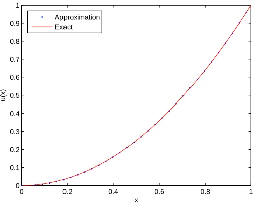
Now, we work with the Cubic RBF ϕ(x) =x3 and the numerical solutions are plotted in Figure 1.As observed Figure 1, numerical results show simplicity and very good accuracy of the persent method. We point out that the corresponding numerical solutions are obtained using Software Matlab.
0 0.2 0.4 0.6 0.8 1
0 0.1 0.2 0.3 0.4 0.5 0.6 0.7 0.8 0.9 1
x
u(x)
Approximation Exact
6. CONCLUSIONS
Meshless methods based on collocation with RBFs for numerical solution of fractional differential equations are investigated in this paper. Numerical results obtained, show high accuracy of the method, as compared with exact solution.We have shown in this work that RBFs can be used to efficiently capture this feature.
Acknowledgements
The authors wish to thank the anonymous referees for their detailed reading of the manuscript and for many useful comments and excellent suggestions that have helped improve the manuscript significantly.
References
1. R.C.Koeller.Application of fractional calculus to the theory of viscoelasticityJ.Appl.Mech,51(1984),229-307. 2. D.A. Benson, S.W. Wheatcraft, and M.M. Meerschaert Application of a fractional advection dispersion
equa-tion,Water Resour.Res,36(2000),1403-1412.
3. R. Goreno, F. Mainardi, E. Scalas, and M. Raberto Fractional calculus and continuous-time finance. III, The diffusion limit. Mathematical finance,Trends in Math.Birkhauser, Basel.(2001),171-180.
4. M. Raberto, E. Scalas, and F. Mainardi,Waiting-times and returns in high-frequency financial data,An empirical study,Phys. A.314( 2002),749-755.
5. I. Podlubny, Fractional Differential Equations,Academic Press,(1999).
6. A.M.A. El-Sayed and M. Gaber,The Adomian decomposition method for solving partial differential equations of fractal order in finite domains,Physics Letters A,359(2006),175-182.
7. H. Jafari and S. Seifi ,Homotopy analysis method for solving linear and nonlinear fractional diffusion-wave equation,Commun. Nonlinear Sci.Numer.Simulat,14,(2009),2006-2012.
8. A.Golbabai, K.Sayevand,Analytical treatment of differential equations with fractional coordinate derivatives.
Computers Mathematics with Applications,62(3)(2011),1003-1012.
9. Momani and Z. OdibatA novel method for nonlinear fractional partialdifferential equations: Combination of DTM and generalized Taylor’s formula,Journal of Computational and Applied Mathematics,220(2008),85-95. 10. S. A. Sarra and E. J. Kansa. Multiquadric Radial Basis Function Approximation Methods for the Numerical
Solution of Partial Differential Equations, Science Press, 2010.
11. MD.Buhmann, Radial Basis Functions: Theory and Implementations,Cambridge University Press,(2003). 12. R.Hardy,Multiquadric equations of topography and other irregular surfaces,Journal of Geophysical
Research,76(8)(1971),1905-1915.
13. R.Franke,Scattered data interpolation:Tests of some methods,Math.Comput,38(157)(1982),181-200.
14. C.Micchelli,Interpolation of scattered data: distance matrices and conditionally positive definite func-tions,Constructive Approximation,2(1)(1986),11-22.
15. B.J.C. Baxter,The Interpolation Theory of Radial Basis Functions,Cambridge University,(1997).
16. G.E Fasshauer, and G. Z JackOn choosing optimal shape parameters for RBF approximation,Numerical Algorithms.45(2007),345-368.
17. A.J. Khattak, S.I.A. Tirmizi, S.U. Islam, Application of meshfree collocation method to a class of nonlinear partial differential equations,Eng. Anal. Bound.Elem,33(2009),661-667.
18. W.Cheney,W.Light, A Course in Approximation Theory, William Allan, New York,(1999).