Estimating the Capacity of the Basic Freeway Section Using Headway Method in Developing Countries (Case Study: Iran

(1)

127 International Journal of Transportation Engineering,

Vol.4/ No.2/ Autumn 2016

Estimating the Capacity of the Basic Freeway Section Using

Headway Method in Developing Countries (Case Study: Iran)

Soheil Sohrabi1_{, Khosrow Ovaici}2_{, Mina Ghanbarikarekani}3

Received: 24.11.2015 Accepted: 16.07.2016

Abstract:

Although there are remarkable differences in drivers’ behavior as well as vehicles characteristics, road capacity esti-mation methods in developing countries are same as developed ones. So, the discrepancy between the theoretical and practical values of capacity is inevitable. Although, capacity estimation methods can be classified based on numerous parameters, in developing countries, the availability of data is a remarkable factor to choose the appropriate method. Headway method is one of the most popular methods which is used to estimate capacity of basic freeways section regarding to the lack of available data in developing countries such as Iran. According to headway method theory, the distribution function of headways needs to be estimated in order to find the capacity of a road facility. However, in previous studies the mean of observed headway is used for capacity estimation.

The data applied in this study have been collected from Iran. Modelling had accomplished in 2 steps: 1) Filtering the input data that are related to following vehicles and just before queue. 2) Statistical modelling using the Minitab 16 software. Evaluating models by three parameters (applicability, validity and reasonability), it was proven that the log -normal distribution functions, is the best fit to observed data. According to results, the capacity of the basic freeway section is 12% less than the values proposed by HCM, which are the current bases for traffic studies in developing countries such as Iran.

Keywords:

Capacity, headway, following vehicle, follower vehicle

Corresponding author E-mail: [email protected]

(2)

128

International Journal of Transportation Engineering, Vol.4/ No.2/ Autumn 2016

1. Introduction

Roadway Capacity estimation is one of the major as-pects in traffic engineering and many studies have been conducted around this subject. Typically capacity esti-mation is based on analysis of significant data bases or is in accordance with theoretical algorithms and Physics laws while some methods are based on simulation re-sults [Roess, Prassas and McShane, 2004]. The capacity and other flow characteristics depend heavily on driver behavior. Although, there are significant differences in drivers’ behavior and vehicles characteristics in devel-oping countries comparing with developed ones, HCM which is developed in United States is used directly for capacity studies around the world [Ashutosh, Senathip-athi and Madhu, 2013]. Consequently, the results are almost unreal in practice and may cause unprofitable constructions. On the other hand, lack of required infra-structures in developing countries leads to insufficient data availability in traffic studies.

According to the aforementioned explanations, in this study, the capacity of freeway for a developing country, Iran, will be estimated in order to investigate possible differences with the HCM proposed values. Differ-ent methods have been proposed for capacity estima-tion like headway methods, maximum observed flow method, probabilistic methods and etc. Considering all aspects such as data requirement, location choice and observation period that are more meaningful in devel-oping countries, time headway method is selected. Es -timating the capacity, on the basis of the models related to headway, is carried out by assuming constant vehicle attitudes. These models are able to estimate the capac-ity of only one lane. Indeed, the assumption of models related to headway, are the separate functions of lane in multi-lane roads. The headway models can be used for one lane in both stable and unstable flow. [Minderhoud, Botma and Bovy, 1996]

According to inverse relation of headway and flow rate, the maximum flow rate, in other words “capacity”, can be estimated using accepted headway of drivers’ in a traffic flow. In this study, drivers’ headway of follower vehicles and before queue is applied. In this case, the abnormal behavior of Iranian drivers in a congested flow will be eliminated. Followers’ vehicles are found by the well-known General Motors’ following model.

In order to estimate the capacity, the headway should be introduced as a deterministic value with the capa-bility of describing the drivers’ behavior. Although in previous studies in Iran the mean headway have been utilized, in this study the estimated distribution function of headways is used for finding the exclusive value of headway [Abtahi, Tamanaiee and Kermanshahi, 2011]. Finding the distribution function of headway is the vital part of this study, where eight well-known distribution functions in traffic studies are fitted to drivers’ headway data of Iran freeways and the best model is introduced. Distribution functions are validated using three param-eters_ applicability, validity and reasonability.

2. Literature Review

The headway attitudes were discussed in 1960s. Green-berg has found a connection between the microscopic traffic flow theory and the lognormal follower head -way distribution [Greenberg, 1966]. Branston 1976 and Buckley 1968 presented the models based on headway. These models are based on following drivers’ data at the time of perceiving the capacity level, and the com-patibility of the hypothesis and the observed data had been proven [Branston, 1976; Buckley, 1968].

Mei and Bullen presented different distribution func-tions for time headways measured on a four-lane high-way. According to their results, the lognormal distribu-tion with a shift of 0.3 or 0.4 seconds was the best fit for the time headways in high traffic volumes [Mei and Bullen, 1993]. Sadeghhosseini in 2002 investigated the time headways at flow rates varying from 140 to 1704 vehicles per hour per lane on a highway and suggest-ed the lognormal distribution [Sadeghhosseini, 2002]. Arasan and Koshy in 2003 determined the negative exponential distribution for headways distribution of urban arterial in India [Arasan and Koshy, 2003]. Bham and Ancha in 2006 analyzed the time headway of driv-ers in a basic freeway section and recommended the lognormal distribution for vehicles’ headway [Bham and Ancha, 2006].

(3)

129 International Journal of Transportation Engineering,

Vol.4/ No.2/ Autumn 2016 ent traffic lanes are the same [Zwahlen, Oner and Sura

-varam, 2007].

In addition to what has been mentioned, the empiri-cal models are other forms of headway models. These models are introduced by cumulative distribution func-tions. Some studies, which were focused on estimating mode, the median and the coefficient of variation have been conducted, that Buckley research in 1968 has been the most reputed one. Also, Breiman et al. in 1977 and Griffiths & Hunt in 1991 have carried out some re -search in this field [Breiman et al., 1977; Griffiths & Hunt, 1991].

It should be considered that the discrepancy between distribution functions and results in different countries and also variety of the proposed models are problems of the presented models. The reason of the mentioned problem is that the drivers’ behavior is completely dif-ferent and their sensitivity impacts on time headway. Also, statistical characteristics of the models have not been presented comprehensively. In empirical models, determining the statistical characteristics of models is complicated and they cannot be generalized. In addi-tion to what is expressed, Luttinen in 1996 investigated these models and demonstrated that the disadvantages of the headway models are interpreting of small data [Luttinen, 1996].

Although, the distribution function is used to model the drivers’ behavior for choosing the time headway in traffic flow, in Iran, capacity is estimated by the mean value of observed headways. [Abtahi, Tamanaiee and Kermanshahi, 2011]

3. Data Collection

In this study 2 types of data, macroscopic and micro-scopic data, are utilized. Macromicro-scopic parameters are mean speed, mean headway and flow, and in the form of microscopic parameters, vehicles speed, vehicle ac-celeration rate have been collected. The data related to macroscopic parameters are collected from the detec-tors which are available in Iran’s freeways. Collected data are available in form of mean headway of 5-minute intervals. According to current limitations in available data in Iran, the microscopic parameters have been col-lected by video-recording and image processing. Selected sections are base sections according to

high-way capacity manual (HCM) definition [TRB 2010] with 3-lanes and 120 km/hr speed limits. According to Base section definition of freeways, there is no access to studying sections. In Iran heavy vehicles are not al-lowed to use freeway facilities.

The total time needed for surveying the macroscopic parameters is considered one year in working days, and the time of surveying the microscopic parameters is 2-hour intervals in morning and evening in working days as well. The users of freeway in working days are commuters which are familiar to the road. All the data were provided in ordinary weather condition and dry pavement conditions.

According to the presented explanations, 3 sections have been selected, and related data will be used in this study.

4. Methodology

The following equations are bases for capacity estima-tion using headway models.

4





n h

hm p

(1)

m h

q 1

(Vehicle per second)

(2)

In these equations

:

p

h

= The time headway between vehicle P and its next vehicle (sec)

m

h

= The mean headway of all the vehicles

q

= The vehicles’ flow rate

n

= The number of vehicles passing the section during time t

As it is obvious from the above equation, capacity i.e. the maximum flows that can

reasonably be estimated by reciprocal of the minimum headway. It would be possible to estimate

the minimum mean headway and the capacity, if the headway distribution of vehicles is

determined as a mathematics model.

In addition,

the vehicles’ headway depends on flow

characteristics. According to

Branston 1976 and Buckley 1968 hypotheses, vehicles at the capacity level cannot maneuver, so

they are following

[Branston, 1976; Buckley, 1968]

. In other words, headway distribution

function at the capacity level, are equal to the following

vehicles’

headway. This hypothesis has

been considered in most of headway models and this study. At the same time, according to

investigations in Iran as a developing country

, the drivers’

behavior is remarkably different in

period of time before queuing. In other word, the headway is significantly small at the time of

queue. Consequently, in this study, the data related to queue, will be eliminated as a new

hypothesis.

4.1

Following Vehicles

The car-following theories represent how vehicles follow others in an uninterrupted flow

and are known as the most common parameters fo

r driver’s

behavior definition. According to

these models, vehicles are categorized in two groups which are following and free. The following

vehicles cannot maneuver or change their direction, and their behavior depend on head vehicles

named

“

leader

”

. However, free vehicles can maneuver and move freely. Different models have

been introduced in this field up to now. According to limited available data in General Motors

Models have been chosen. [Tom and Krishna Rao, 2004]

General Motors presents the car-following definition regarding

two assumptions: 1)

The

higher speed the more distance, 2) Heeding to safe [Tom and Krishna Rao, 2004]

. The maximum

following time can be estimated by using the equations which have been presented by General

Motors. The equation 3

can be presented as:

[Tom and Krishna Rao, 2004]

t n v safe x t

n

x _₁  _₁

 

(3)

Differentiating the above equation with respect to time,

t n a t

n v t n

v  _₁ _₁

(4)

In this equation:

t n x _₁



= The distance between the (n+1) vehicle and previous vehicle in t

th

second

(meters)

safe x



= Safe space distance in t

th

second (meters)

(1)

4





n h

hm p

(1)

m h

q 1

(2)

In these equations

:

p

h

m

h

q

n

= The number of vehicles passing the section during time t

reasonably be estimated by reciprocal of the minimum headway. It would be possible to estimate

In addition,

the vehicles’ headway depends on flow

they are following

. In other words, headway distribution

vehicles’

been considered in most of headway models and this study. At the same time, according to

, the drivers’

period of time before queuing. In other word, the headway is significantly small at the time of

hypothesis.

4.1

Following Vehicles

The car-following theories represent how vehicles follow others in an uninterrupted flow

r driver’s

named

“

leader

”

been introduced in this field up to now. According to limited available data in General Motors

two assumptions: 1)

The

. The maximum

Motors. The equation 3

t n v safe x t

n

x _₁  _₁

 

(3)

t n a t

n v t n

v  _₁ _₁

(4)

In this equation:

t n x _₁



th

second

(meters)

safe x



th

second (meters)

(Vehicle per second) (2)

In these equations:

hp = The time headway between vehicle P and its next

vehicle (sec)

hm = The mean headway of all the vehicles

q = The vehicles’ flow rate

n = The number of vehicles passing the section during time t

As it is obvious from the above equation, capacity i.e. the maximum flows that can reasonably be estimated by reciprocal of the minimum headway. It would be possible to estimate the minimum mean headway and the capacity, if the headway distribution of vehicles is determined as a mathematics model.

(4)

130

International Journal of Transportation Engineering, Vol.4/ No.2/ Autumn 2016

in most of headway models and this study. At the same time, according to investigations in Iran as a developing country, the drivers’ behavior is remarkably different in period of time before queuing. In other word, the head-way is significantly small at the time of queue. Conse -quently, in this study, the data related to queue, will be eliminated as a new hypothesis.

4.1 Following Vehicles

The car-following theories represent how vehicles fol-low others in an uninterrupted ffol-low and are known as the most common parameters for driver’s behavior defi -nition. According to these models, vehicles are catego-rized in two groups which are following and free. The following vehicles cannot maneuver or change their direction, and their behavior depend on head vehicles named “leader”. However, free vehicles can maneuver and move freely. Different models have been introduced in this field up to now. According to limited available data in General Motors Models have been chosen. [Tom and Krishna Rao, 2004]

General Motors presents the car-following definition regarding two assumptions: 1) The higher speed the more distance, 2) Heeding to safe [Tom and Krishna Rao, 2004]. The maximum following time can be esti -mated by using the equations which have been present-ed by General Motors. The equation 3 can be presentpresent-ed as: [Tom and Krishna Rao, 2004]

4





n h

hm p

(1)

m h

q 1

(2)

In these equations

:

p

h

m

h

q

n

= The number of vehicles passing the section during time t

reasonably be estimated by reciprocal of the minimum headway. It would be possible to estimate

In addition,

the vehicles’ headway depends on flow

they are following

. In other words, headway distribution

vehicles’

been considered in most of headway models and this study. At the same time, according to

, the drivers’

period of time before queuing. In other word, the headway is significantly small at the time of

hypothesis.

4.1

Following Vehicles

The car-following theories represent how vehicles follow others in an uninterrupted flow

r driver’s

named

“

leader

”

been introduced in this field up to now. According to limited available data in General Motors

two assumptions: 1)

The

. The maximum

Motors. The equation 3

t n v safe x t n

x _₁  _₁

 

(3)

t n a t n v t n

v  _₁ _₁

(4)

In this equation:

t n x _₁



th

second

(meters)

safe x



th

second (meters)

(3)

4





n h

hm p

(1)

m h

q 1

(2)

In these equations

:

p

h

m

h

q

n

= The number of vehicles passing the section during time t

reasonably be estimated by reciprocal of the minimum headway. It would be possible to estimate

In addition,

the vehicles’ headway depends on flow

they are following

. In other words, headway distribution

vehicles’

been considered in most of headway models and this study. At the same time, according to

, the drivers’

period of time before queuing. In other word, the headway is significantly small at the time of

hypothesis.

4.1

Following Vehicles

The car-following theories represent how vehicles follow others in an uninterrupted flow

r driver’s

named

“

leader

”

been introduced in this field up to now. According to limited available data in General Motors

two assumptions: 1)

The

. The maximum

Motors. The equation 3

t n v safe x t n

x _₁  _₁

 

(3)

t n a t n v t n

v  _₁ _₁

(4)

In this equation:

t n x _₁



th

second

(meters)

safe x



th

second (meters)

(4)

In this equation:

4



 n

h

hm p (1)

m

h

q 1 (Vehicle per second) (2)

In these equations:

p

h = The time headway between vehicle P and its next vehicle (sec)

m

h = The mean headway of all the vehicles q = The vehicles’ flow rate

In addition, the vehicles’ headway depends on flow characteristics. According to Branston 1976 and Buckley 1968 hypotheses, vehicles at the capacity level cannot maneuver, so they are following [Branston, 1976; Buckley, 1968]. In other words, headway distribution function at the capacity level, are equal to the following vehicles’ headway. This hypothesis has been considered in most of headway models and this study. At the same time, according to investigations in Iran as a developing country, the drivers’ behavior is remarkably different in period of time before queuing. In other word, the headway is significantly small at the time of queue. Consequently, in this study, the data related to queue, will be eliminated as a new hypothesis.

4.1Following Vehicles

The car-following theories represent how vehicles follow others in an uninterrupted flow and are known as the most common parameters for driver’s behavior definition. According to these models, vehicles are categorized in two groups which are following and free. The following vehicles cannot maneuver or change their direction, and their behavior depend on head vehicles named “leader”. However, free vehicles can maneuver and move freely. Different models have been introduced in this field up to now. According to limited available data in General Motors Models have been chosen. [Tom and Krishna Rao, 2004]

General Motors presents the car-following definition regarding two assumptions: 1) The higher speed the more distance, 2) Heeding to safe [Tom and Krishna Rao, 2004]. The maximum following time can be estimated by using the equations which have been presented by General Motors. The equation 3 can be presented as: [Tom and Krishna Rao, 2004]

t n v safe x t n

x _₁  _₁

  (3)

t n a t n v t n

v  _₁ _₁ (4)

In this equation: t

n

x _₁

 = The distance between the (n+1) vehicle and previous vehicle in tth second (meters)

safe x

 = Safe space distance in tth second (meters)

= The distance between the (n+1) vehicle and previous vehicle in tth_{second (meters)}

4



 n h h p

m (1)

m

h

In these equations:

p

m

4.1Following Vehicles

t n v safe x t n

x _₁  _₁

  (3)

t n a t n v t n

v  _₁ _₁ (4)

In this equation: t

n

x _₁

safe x

= Safe space distance in tth_{second (meters)}

4



 n

h

hm p (1)

m

h

In these equations:

p

m

4.1Following Vehicles

t n v safe x t n

x _₁  _₁

  (3)

t n a t n v t n

v  _₁ _₁ (4)

In this equation: t

n

x _₁

safe x

= (n+1) vehicle’s speed in tth_{second (meters per}

second)

5

t n

v _₁= (n+1) vehicle’s speed in tth_{second (meters per second)}

= Driver’s sensitivity coefficient (seconds) t

n

a _₁= (n+1) vehicle’s acceleration rate in tth second (meters per second squared) The decision distance of the following vehicle will be considered as the desired distance if the speed of the leader vehicle is reduced. Therefore, the following time distance can be estimated by equation 5.

  T_safe f

T (5)

In this equation:

f

T =The desired time distance (seconds)

safe

T =The safe time distance (seconds)

The safe time distance in equation 5 is the reaction time. Thus, the desired time distance can be estimated by calculating the sensitivity coefficient of driver. The sensitivity coefficient of driver will be counted by equation 4 and using collected microscopic data. Vehicles with greater headway than estimated desired time distance are assumed as free vehicles.

4.2Queuing

Since the vehicles headway at the capacity level has been considered, and there is remarkable discrepancy between drivers’ behavior before and after queuing, the data related to queue have to be eliminated. In order to recognizing and eliminating the relevant data, the speed-flow diagram is used. Indeed, speed-flow drop i.e. breakdown, and its relevant speed is the best factor for the queue recognition [Chung, Rudjanakanoknad and Cassidy, 2007; Dowling et al., 1997]. The speed-flow curves have been suggested for the sake of finding the speed corresponded to breakdown [Maerivoet and De Moor, 2008].

4.3Mathematical Modelling

The hypothesis of statistical modelling is based on accidental input data with no trend [Luttinen 1996]. Three tests suggested for determining data trend are: 1) Weighted sign test, 2) Kendall rank correlation test and 3) exponential ordered scores test. In order to trend data, correlation tests are utilized. The pair data are compared in this test [Stuart and Ord 1991]. Because of the complicated calculations, statistical software is used. It has to be considered that, generally, traffic data has a specific trend [Luttinen, 1996].

The model parameters are estimated after investigating the data trend. The model parameters estimation is the most vital step in statistical modelling. These parameters can be estimated by several methods. The most well- known methods of model parameters analysis are Moments method, Maximum likelihood and Chi-square. The most common method of parameter estimation is Maximum likelihood [Luttinen, 1996].

5. Modeling Procedure

The headway data modeling is conducted in two steps which are: preparing and filtering the input data and statistical modelling. In first step, the input data for the follower vehicles before the queuing have filtered using the following time criteria and related speed of flow drop.

In second step, the statistical models, related to vehicles’ headway for each freeways lane have been estimated.

5.1First step: Preparing Input Data = Driver’s sensitivity coefficient (seconds)

5

t n

n

T (5)

In this equation:

f

safe

T =The safe time distance (seconds) The safe time distance in equation 5 is the reaction time. Thus, the desired time distance can be estimated by calculating the sensitivity coefficient of driver. The sensitivity coefficient of driver will be counted by equation 4 and using collected microscopic data. Vehicles with greater headway than estimated desired time distance are assumed as free vehicles.

4.2Queuing

5. Modeling Procedure

5.1First step: Preparing Input Data

= (n+1) vehicle’s acceleration rate in tth_second

(meters per second squared)

The decision distance of the following vehicle will be considered as the desired distance if the speed of the

leader vehicle is reduced. Therefore, the following time distance can be estimated by equation 5.

5

t n

n

T (5)

In this equation:

f

safe

T =The safe time distance (seconds)

The safe time distance in equation 5 is the reaction time. Thus, the desired time distance can be estimated by calculating the sensitivity coefficient of driver. The sensitivity coefficient of driver will be counted by equation 4 and using collected microscopic data. Vehicles with greater headway than estimated desired time distance are assumed as free vehicles.

4.2Queuing

5. Modeling Procedure

5.1First step: Preparing Input Data

(5)

In this equation:

Tf = The desired time distance (seconds)

Tsafe =The safe time distance (seconds)

The safe time distance in equation 5 is the reaction time. Thus, the desired time distance can be estimated by calculating the sensitivity coefficient of driver. The sensitivity coefficient of driver will be counted by equa -tion 4 and using collected microscopic data. Vehicles with greater headway than estimated desired time dis-tance are assumed as free vehicles.

4.2 Queuing

Since the vehicles headway at the capacity level has been considered, and there is remarkable discrepancy between drivers’ behavior before and after queuing, the data related to queue have to be eliminated. In or-der to recognizing and eliminating the relevant data, the speed-flow diagram is used. Indeed, flow drop i.e. breakdown, and its relevant speed is the best factor for the queue recognition [Chung, Rudjanakanoknad and Cassidy, 2007; Dowling et al., 1997]. The speed-flow curves have been suggested for the sake of finding the speed corresponded to breakdown [Maerivoet and De Moor, 2008].

4.3 Mathematical Modelling

The model parameters are estimated after investigating the data trend. The model parameters estimation is the most vital step in statistical modelling. These param-eters can be estimated by several methods. The most well- known methods of model parameters analysis are Moments method, Maximum likelihood and

(5)

131 International Journal of Transportation Engineering,

Vol.4/ No.2/ Autumn 2016

square. The most common method of parameter estima-tion is Maximum likelihood [Luttinen, 1996].

5. Modeling Procedure

The headway data modeling is conducted in two steps which are: preparing and filtering the input data and statistical modelling. In first step, the input data for the follower vehicles before the queuing have filtered us -ing the follow-ing time criteria and related speed of flow drop. In second step, the statistical models, related to vehicles’ headway for each freeways lane have been estimated.

5.1 First Step: Preparing Input Data

Filtering Free Vehicles

Drivers’ reaction time in Iran has been investigated by Sohrabi et al. in Hamedan Medical University. This study has been carried out on 46 individuals (including 10 females and 36 males) and has been complemented on each volunteer using a simulator machine for one hour. The sample contains includes drivers with driv-ing license who drive both professionally and unprofes-sionally. Also, includes variety of age, gender and driv-ing experience. The drivers’ reaction has been recorded has been analyzed by SPSS software in next step. Re -sults have demonstrated that the mean reaction time of decelerating is 1320 milliseconds. Also, the time of releasing the accelerator has been estimated 559

mil-liseconds [Sohrabi et al., 2013].

If the driver’s reaction time is considered as the sum of perception, decision and action time [Elefteriadou 2014], the sum of releasing accelerator pedal and pushing on the decelerating pedal will be equal to the driver’s reaction time. Consequently, the driver’s reac-tion time in Iran has been determined 1879 millisec-onds.

The equation 5 is used to estimate the driver’s sensi-tivity coefficient. vt

n, vtn+1 and atn+1 have been collected

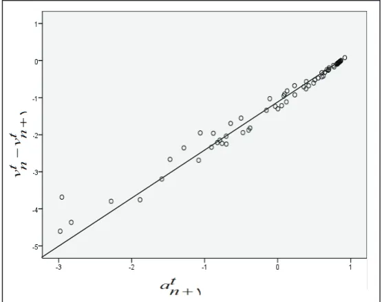
and analyzed as microscopic data which is discussed before. In next step, the sensitivity coefficient has been estimated using regression model. Modelling process has been done using SPSS. The linear regres-sion model with zero constant value has been applied and result is shown in equation 6 and Figure 1.

6

Filtering Free Vehicles

Drivers’ reaction time in Iran has been investigated by Sohrabi et al. in Hamedan Medical University. This study has been carried out on 46 individuals (including 10 females and 36 males) and has been complemented on each volunteer using a simulator machine for one hour. The sample contains includes drivers with driving license who drive both professionally and unprofessionally. Also, includes variety of age, gender and driving experience. The drivers’

reaction has been recorded has been analyzed by SPSS software in next step. Results have demonstrated that the mean reaction time of decelerating is 1320 milliseconds. Also, the time of releasing the accelerator has been estimated 559 milliseconds [Sohrabi et al., 2013].

If the driver’s reaction time is considered as the sum of perception, decision and action time [Elefteriadou 2014], the sum of releasing accelerator pedal and pushing on the decelerating pedal will be equal to the driver’s reaction time. Consequently, the driver’s reaction time in Iran

has been determined 1879 milliseconds.

The equation 5 is used to estimate the driver’s sensitivity coefficient. vt_n,v_nt_₁andat_n_₁

have been collected and analyzed as microscopic data which is discussed before. In next step, the sensitivity coefficient has been estimated using regression model. Modelling process has been done using SPSS. The linear regression model with zero constant value has been applied and result is shown in equation 6 and Figure 1.

t n a t

n v t n

v  _₁1.646 _₁ (6)

Figure 1.The Equation of Estimated Regression in order to Determining the Driver’s Sensitivity Coefficient

According to outputs, the corrected R2_{has been determined 0.933. Also, as is presented} is Table 1, related P-values of model and independent variable are zero, which means, the model and independent variable are significant with 95% confidence.

Table 1. Results of model statistical tests

Model Independent Variable Independent

Variable Coefficient

Corrected R2 _{P-Value Model (F)} _P-Value

0.933 0.00 0.00 1.646

(6) According to outputs, the corrected R2 has been deter-mined 0.933. Also, as is presented is Table 1, related P-values of model and independent variable are zero, which means, the model and independent variable are significant with 95% confidence.

As it was mentioned, the desired time distance is sum of the reaction time and driver’s sensitivity coefficient. Therefore, this value is determined as 3.525, which is meant the vehicles that have time headway less than 3.525 are follower vehicles and the others are free ones. Free vehicles have been eliminated for data base.

6

Filtering Free

Vehicles

Drivers’ reaction time in Iran has been investigated by Sohrabi et al.

in Hamedan Medical

University. This study has been carried out

on 46 individuals (including 10 females and 36

males) and has been complemented on each volunteer using a simulator machine for one hour.

The sample contains includes drivers with driving license who drive both professionally and

unprofessionally. Also, includes variety of age, gender and driving

experience

. The

drivers’

reaction has been recorded has been analyzed

by SPSS software in next step.

Results have

demonstrated that the mean reaction time of decelerating is 1320 milliseconds. Also, the time of

releasing the accelerator has been estimated 559 milliseconds [Sohrabi et al., 2013].

If the driver’s reaction time

is considered as the sum of perception, decision and action

time [

Elefteriadou

2014], the sum of releasing accelerator pedal and pushing on the decelerating

pedal

will be equal to the driver’s reaction time. Consequently, the driver’s reaction time in Iran

The equation 5 is used to estimate

the driver’s sensitiv

ity coefficient.

vt_n

,

v_nt _₁

and

at_n_₁

have been collected and analyzed as microscopic data which is discussed before

. In next step,

the sensitivity coefficient has been estimated using regression model. Modelling process has

been done using SPSS. The linear regression model with zero constant value has been applied

and result is shown in equation 6 and Figure 1.

t n a t

n v t n

v  _₁1.646 _₁

(6)

According to outputs, the corrected R

2

has been determined 0.933. Also, as is presented

is Table 1, related P-values of model and independent variable are zero, which means, the model

and independent variable are significant with 95% confidence.

Model Independent Variable Independent

0.933 0.00 0.00 1.646

(6)

132

International Journal of Transportation Engineering, Vol.4/ No.2/ Autumn 2016

Table 1. Results of model statistical tests

Filtering queue data

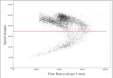
Speed and flow data of the study section are fitted for 5- minute periods as shown in Figure 2. The data is collected for one year period of study section (almost 100,000 observations) and each point represents an ob-servation.

As it is depicted, flow drop have been occurred in flow speed 68 kilometers per hour, where the data density is re-duced. In consequence, the data with mean speed more than 68 kilometers per hour have been utilized in this study.

5.2 Second Step: Modelling

In this step, the filtered data have been extracted accord -ing to maximum vehicles’ headway and minimum ve -hicles’ mean speed, and modelling has been conducted by statistical software, Minitab16. The trendless feature of data has been examined using correlation method as mentioned before. Finally, modelling has been carried out for each lane and the entire section and model’s parameters have estimated. (Table 2 to 5) Eight

well-known distribution functions in traffic studies are uti -lized to find the best fitted model of observed headway.

6. Evaluation Models

In order to find the best distribution function, models have been evaluated by three criteria and the best model has been presented.

6.1 Applicability

The applicable model should have not only simple structure and definition, but also specific statistical at -titudes. In addition, this model can be reviewed and the model parameters can be estimated. Therefore, the well-known statistical models in this study are consid-ered and experimental models are not investigated. According to the conducted studies up to now, in this study 4 models are investigated. These 4 models are: 1- Normal distribution function and exponential distri -bution function

2- Lognormal distribution function and 3-parameter 6

Filtering Free

Vehicles

Drivers’ reaction time in Iran has been investigated by Sohrabi et al.

in Hamedan Medical

University. This study has been carried out

on 46 individuals (including 10 females and 36

males) and has been complemented on each volunteer using a simulator machine for one hour.

The sample contains includes drivers with driving license who drive both professionally and

unprofessionally. Also, includes variety of age, gender and driving

experience

. The

drivers’

reaction has been recorded has been analyzed

by SPSS software in next step.

Results have

demonstrated that the mean reaction time of decelerating is 1320 milliseconds. Also, the time of

releasing the accelerator has been estimated 559 milliseconds [Sohrabi et al., 2013].

If the driver’s reaction time

is considered as the sum of perception, decision and action

time [

Elefteriadou

2014], the sum of releasing accelerator pedal and pushing on the decelerating

pedal

will be equal to the driver’s reaction time. Consequently, the driver’s reaction time in Iran

The equation 5 is used to estimate

the driver’s sensitiv

ity coefficient.

v_nt

,

v_nt _₁

and

at_n_₁

have been collected and analyzed as microscopic data which is discussed before

. In next step,

the sensitivity coefficient has been estimated using regression model. Modelling process has

been done using SPSS. The linear regression model with zero constant value has been applied

and result is shown in equation 6 and Figure 1.

t n a t

n v t n

v  _₁1.646 _₁

(6)

According to outputs, the corrected R

2

has been determined 0.933. Also, as is presented

is Table 1, related P-values of model and independent variable are zero, which means, the model

and independent variable are significant with 95% confidence.

Model Independent Variable Independent

0.933 0.00 0.00 1.646

7

As it was mentioned, the desired time distance

is sum of the reaction time and driver’s

sensitivity coefficient. Therefore, this value is determined as 3.525, which is meant the vehicles

that have time headway less than 3.525 are follower vehicles and the others are free ones. Free

vehicles have been eliminated for data base.

Filtering queue data

Speed and flow data of the study section are fitted for 5- minute periods as shown in

Figure 2. The data is collected for one year period of study section (almost 100,000 observations)

and each point represents an observation.

Figure 2. Flow-speed diagram of study section

As it is depicted, flow drop have been occurred in flow speed 68 kilometers per hour,

where the data density is reduced. In consequence, the data with mean speed more than 68

kilometers per hour have been utilized in this study.

5.2

Second Step: Modelling

In this step, the filtered data

have been extracted according to maximum vehicles’

headway and minimum vehicles’ mean speed, and

modelling has been conducted by statistical

software, Minitab16. The trendless feature of data has

been examined using correlation method

as mentioned before. Finally, modelling has been carried out for each lane and the entire section

and model’s parameters have estimated. (Table 2 to 5) Eight well

-known distribution functions

in traffic studies are utilized to find the best fitted model of observed headway.

Spe

ed (kmph)

Flow Rate (veh per 5 min)

Figure 2. Flow-speed diagram of study section

(7)

133 International Journal of Transportation Engineering,

Vol.4/ No.2/ Autumn 2016

Table 2. Parameters of the headway model for first lane data

Table 3. Parameters of the headway model for second lane data

Table 4. Parameters of the headway model for third lane data

8

Table 2. Parameters of the headway model for first lane data

Parameters Model Threshold Scale Shape Location NA 0.146 11.067 NA Gamma 0.928 0.368 1.881 NA

3- parameter Gamma

NA 0.549 NA 1.620 Normal NA 1.620 NA NA Exponential NA 0.289 0.437 NA Lognormal 0.217 0.316 0.049 NA

3- parameter Lognormal

NA 1.810 2.928 NA Weibull 0.935 0.752 1.354 NA

3- parameter Weibull

NA = Not available.

Table 3. Parameters of the headway model for second lane data

3- parameter Gamma

NA 2.212 2.997 NA Weibull 0.875 1.245 1.754 NA

NA = Not available.

Table 4. Parameters of the headway model for third lane data

Parameters Model Threshold Scale Shape Location NA 0.228 1196315 NA Gamma -7.450 0.056 181.804 NA

3- parameter Gamma

NA 3.012 4.373 NA Weibull -3.077 6.132 9.493 NA

NA = Not available.

8

3- parameter Gamma

NA 1.810 2.928 NA Weibull 0.935 0.752 1.354 NA

NA = Not available.

3- parameter Gamma

NA 2.212 2.997 NA Weibull 0.875 1.245 1.754 NA

NA = Not available.

3- parameter Gamma

NA 3.012 4.373 NA Weibull -3.077 6.132 9.493 NA

NA = Not available.

8

3- parameter Gamma

NA 1.810 2.928 NA Weibull 0.935 0.752 1.354 NA

NA = Not available.

3- parameter Gamma

NA 2.212 2.997 NA Weibull 0.875 1.245 1.754 NA

NA = Not available.

3- parameter Gamma

NA 3.012 4.373 NA Weibull -3.077 6.132 9.493 NA

NA = Not available.

(8)

134

International Journal of Transportation Engineering, Vol.4/ No.2/ Autumn 2016

lognormal distribution function

3- Weibull distribution function and 3-parameter weibull distribution function

4- Gamma distribution function and 3-parameter gam-ma distribution function

6.2 Validity

In modelling, validating models is the most prominent step. In this study, the models’ goodness of fit is investigat -ed and the best model will be determin-ed. The goodness of fit tests can be applied in order to investigating the hypoth -esis of equality in observed data distribution with specific distribution. The zero hypothesis of this test (H0) depicts the equality of fitted distribution function on observed data and the reputed distribution function. The contrast hypoth-esis (HA) illustrates the difference of the models.

In order to testing the goodness of fit, several tests have been proposed: Chi- Square test, Kolmogorov- Smirnov and Anderson & Darling tests are widely used in statisti-cal studies. Although all the methods have equal hypoth-eses, it has been demonstrated that Anderson & Darling test (A-D) will have better results concerning to headway data essence. In this method, the maximum value will be estimated as the difference of model and observed data distribution function. This discrepancy is belonged to middle part of function and the discrepancies are slight in beginning and ending part of the function. These discrep-ancies are weighted according to the location in function which each point has specific weight [Luttinen 1996]. In this study, the A-D method will be applied in order to calculating the model goodness of fit. Table 6, presented the goodness of fit of estimated models.

Table 5. Parameters of the Headway Model for the EntireSection

9

Table 5. Parameters of the Headway Model for the EntireSection

Parameters Model

Threshold Scale

Shape Location

NA 0.187

9.644 NA

Gamma

0.874 0.391

2.368 NA

3- parameter Gamma

NA 0.638

NA 1.800

Normal

NA 1.800

NA NA

Exponential

NA 0.314

0.535 NA

Lognormal

0.352 0.342

-0.122 NA

NA 2.016

2.859 NA

Weibull

0.877 1.033

1.556 NA

NA = Not available.

6.

Evaluation Models

In order to find the best distribution function, models have been evaluated by three

criteria and the best model has been presented.

6.1

Applicability

The applicable model should have not only simple structure and definition, but also

specific statistical attitudes. In addition, this model can be reviewed and the model parameters

can be estimated. Therefore, the well-known statistical models in this study are considered and

experimental models are not investigated.

According to the conducted studies up to now, in this study 4 models are investigated.

These 4 models are:

1- Normal distribution function and

exponential

distribution function

2- Lognormal distribution function and 3-parameter lognormal distribution function

3- Weibull distribution function and 3-parameter weibull distribution function

4- Gamma distribution function and 3-parameter gamma distribution function

6.2

Validity

In modelling, validating models is the most

prominent step. In this study, the models’

goodness of fit is investigated and the best model will be determined. The goodness of fit tests

can be applied in order to investigating the hypothesis of equality in observed data distribution

with specific distribution. The zero hypothesis of this test (H

0

) depicts the equality of fitted

distribution function on observed data and the reputed distribution function. The contrast

hypothesis (H

A

) illustrates the difference of the models.

In order to testing the goodness of fit, several tests have been proposed

: Chi

- Square test,

Kolmogorov- Smirnov and Anderson & Darling tests are widely used in statistical studies.

Although all the methods have equal hypotheses, it has been demonstrated that Anderson &

Darling test (A-D) will have better results concerning to headway data essence. In this method,

the maximum value will be estimated as the

difference of model and observed data distribution

function. This discrepancy is belonged to middle part of function and the discrepancies are slight

in beginning and ending part of the function. These discrepancies are weighted according to the

location in function which each point has specific weight [Luttinen 1996]. In this study, the

A-D method will be applied in order to calculating the model goodness of fit. Table 6, presented

the goodness of fit of estimated models.

10

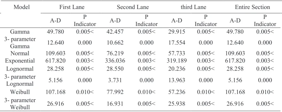
Table 6. The Goodness of Fit of Headway Models

Entire Section third Lane

Second Lane First Lane

Model

P Indicator A-D

0.005> 49.780

0.005> 29.915

0.005> 42.457

0.005> 49.780

Gamma

0.000 12.640

0.000 17.554

0.000 10.662

0.000 12.640

3- parameter Gamma

0.005> 109.603

0.005> 57.733

0.005> 76.219

0.005> 109.603

Normal

0.003> 617.820

0.003> 319.189

0.003> 336.036

0.003> 617.820

Exponential

0.005> 28.258

0.005> 20.236

0.005> 28.550

0.005> 28.258

Lognormal

0.000 5.156

0.000 13.963

0.000 3.731

0.000 5.156

0.010> 107.168

0.010> 57.236

0.010> 77.992

0.010> 107.168

Weibull

0.005> 26.916

0.005> 25.938

0.005> 16.931

0.005> 26.916

As it is obvious, the 3-parameter gamma and 3-parameter lognormal present acceptable

results with 95% confidence level. Indeed, the zero hypotheses is not rejected in these models.

Comparing the A-D value of these two models demonstrates that the 3-parameter lognormal can

present more compatible results than other data.

6.3

Reasonability

Concerning to statistical data characteristics and traffic flow theory, the obtained model

should be compatible to users’

behavior. The last step of headway modelling is investigating the

models with the purpose of

compatibility to drivers’

behavior. As discussed before, both log

normal and gamma distribution have been used in previous traffic studies which satisfies the

reasonability criteria.

7.

Conclusion

In this study, using headway method, capacity of the basic freeway section was

determined. Therefore, headway distribution functions estimated for each freeway lanes. The

essential data of the Iran’s freeways

were collected and the

filtered according to 2 assumptions:

1) the following vehicles, and 2) before queuing. Finally, modelling for function determination

was done by mathematics methods and the models were analyzed

on basis of 3 factors: 1)

Applicability, 2) Validity, and 3) Reasonability. At last, the lognormal model is introduced as

the best distribution function of the headway data for first, second, third lanes and the entire

section.

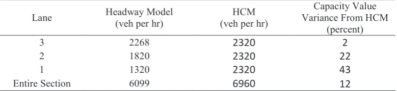
According to the relation of headway and flow rate, the capacity values have been

estimated for each lane and the entire section for a 3-lane freeway basic section as. On the other

hand, the capacity proposed value of HCM under basic section condition and considering the

ratio of buses, is depicted in Table 7.

Table 7. Capacity of Each Lane and the Entire Section for a 3-Lane Freeway basic Section

Lane Headway Model _{(veh per hr)} _(ve