Cluster Based Data Gathering in Wireless Sensor Network

(1)

Cluster Based Data Gathering in Wireless Sensor Network

Abhay Kumar Mishra1,$, Prof. Surendra Mishra2,# Department of Computer science, S.S.S.I.S.T, Sihore (M.P), India E-mail:$abhaymishra4@yahoo.co.in,#smishra1lnct@gmail.com

Abstract—In this paper, clustering in terms of energy efficiency in WSN is explored and proposed Energy Balanced Clustering in Wireless Sensor Network (EBC). Algorithms for energy balanced cluster formation, cluster head selection, intra cluster and inter cluster communication in WSN are proposed. Furthermore, using ns2 simulation performance of proposed protocol is compared with LEACH and EEMC using parameters like energy per packet and throughput. Simulation results demonstrate that EBC is efficient in prolonging the network lifetime as well as in improving throughput, than LEACH and EEMC. In this technique tree is formed inside each cluster and data flows from leaf node to root and finally to the sink.

Index Terms—WSN, EBC, LEACH, EEMC, NS2.

1. Introduction

Sensor networks are wireless networks consisting of a large number of miniature electromechanical devices (sensors) with sensing, computing and communication capabilities [1]-[ 2]. They can be used for collecting sensory information, such as temperature measurements, from an extended geographic area. Operating a sensor network poses algorithmic challenges due to the limited capabilities of the sensor devices. In data gathering problems the focus is in maximizing the amount of data gathered from the sensors to a base station using direct or multi-hop radio transmission, under one or more limiting factors. We have studied data gathering in energy constrained sensor networks. Each sensor operates on battery energy, and the battery is not replenished during the operation. Energy is consumed both in radio transmission and reception. This imposes a number of energy constraints, one for each sensor. Such problems are often formulated in terms of maximizing the total quantity of data gathered, no matter how unevenly it may be divided between the sensors (e.g. [3]-[ 6]). In contrast, we propose a utility function that accommodates both total quantity and fairness (collecting roughly equal quantities from every sensor). Recent developments in processor, memory and radio technology have enabled wireless sensor network which are deployed to collect useful information from an area of interest. The sensed data must be gathered and transmitted to a base station where it is further processed for end-user queries. Since the network consists of low-cost nodes with limited battery power, power efficient methods must be employed for data gathering and aggregation in order to achieve long network lifetimes. In an environment where ina round of communication each of the sensor nodes has data to send to a base station, it is important to minimize the total energy consumed by the system in a round so that the system lifetime is maximized. With the use of data fusion and aggregation techniques, while minimizing the total energy per round, if power consumption per node can be balanced as well, a near optimal data gathering and routing scheme can be achieved in terms of network lifetime. Several application specific sensor network data gathering protocols have been proposed in research literatures. However, most of the proposed algorithms have been some attention to the related network lifetime and saving energy

are two critical issues for wireless sensor networks.

1. Design

The WSN network architecture is shown in Fig. 3. WSNs consist of a large set of autonomous wireless sensing nodes. (Akyildiz et al., 2002) These sensor nodes are randomly deployed in the sensing field. Each sensor node has the ability to detect the target signal, process data, and communicate with other nodes. The nodes transmit their data to the sink, which collects this data periodically. After a predesignated period, the sink will transfer the collected data to the end users via a Local Area Network, the internet, or satellite network. The sensor node hardware consists of four main components. These are the sensing unit, processing unit, communication unit, and power unit. The Analog digital converter (ADC) is a translator that tells the processing unit what the sensor unit has sensed and also informs the sensor unit what to do. The communication unit task is to receive commands or queries. It is also in charge of all communications between the sensor node and sink. The processing unit is responsible for executing the pre-stored program code or coded instructions announced by the sink. It can start up, control, and coordinate the different units in the inner component Much research has been conducted in the low power radio area. Previous research provides assumptions about the radio characteristics and describes the advantages of different protocols and applications. Some research used first order radio modules, in which a fixed dissipating energy, Eelec, is spent in transmitting and receiving a packet of signals[5]. The extra cost is proportional to d2 and is spent on the amplifier Eamp, in transmitting a packet. The equations used to calculate the transmission and receiving costs to transmit a k bit message for a distance d are shown in the following.

Transmitting:

ETx(k, d) = ETx-elec(k) + ETx-amp(k, d) ETx(k, d) = E elec * k + E amp * k * d 2 (1) Receiving:

ERx(k) = ERx-elec(k) ERx(k) = Eelec * (k) (2)

(2)

As shown in Table 1, this model assumes the radio dissipates Eelec = 50 nJ/bit for the Transmitter and Receiver electronics. The Transmit Amplifier dissipation is Eamp = 100 pJ/bit/m2. There is a cost of 5 nJ/bit/message for k = 2000 bit messages in data fusion. It also assumes that the radio channel is symmetrical. This means that the energy required to transmit a message from nodea to nodeb is the same as the energy required to transmit a message from nodeb to nodea for a given signal-to-noise ratio (SNR). The greater the communication power, the greater the SNR and a typical SNR value is 10dB.

2. Implementation

Cluster Establishment [6] (i) Cluster Head Selection [7]

The sink will obtain the node information table with the location and remnant power. We can find the distance between any two nodes using Eq. (3). The coordinates for any two nodes are (xi, yi) and (xj, yj):

d= sqrt((xi–xj)2 + (xi–xj)2 ), (3)

where d is the distance between two nodes and (xi, yi) and (xj, yj) are any two nodes’ coordinates, respectively. We can determine Eq. (1) when the distance, d, between nodes is known. The power dissipation of the transmitter amplifier is constant, 100 pJ/bit/m. The packet size, k, is fixed. We can then compute the power consumption, Ents(k, d), for the node transmission data to the sink one time. The dissipation energy for nodes sending data to the sink is Ents(k, d), which is obtained using Eq. (1). The threshold power value is Eth(k, d) = (t/ar) * Ents(k,d). t, and defines the number of times a node can send data, which is determined by the user. a is a value that limits the time and it is also determined by the user while r represents the time required for building the tree. The sink will compute the remaining power for each node according to that node’s information table and will then determine which nodes will be cluster heads. Each node computes the distance from the sink to itself in turn. The sink also computes the remaining power if it is less than the minimum power needed for sending data to the sink. The threshold power is Eth(k, d). If the remaining power is less than the threshold value, the node will not be a cluster head and the sink will continue to look for a cluster head in turn according to the distance. The sink keeps selecting cluster heads until the number of cluster heads is enough for the WSN. The cluster number, c, can also be tuned by the user according to the number of nodes in the topology.

Figure 2

(ii) Establishing Clusters

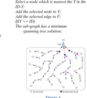
After selecting the cluster heads, the sink computes the distance between the cluster heads and sensor nodes according to the coordinate information. Each node will then be chosen to join the cluster head by cluster. The sensor nodes will compare the distance with each cluster head and will then label the node’s identity and that it has been selected to join a specific cluster. The cluster head plays an important role like a controller. It is also a root node for the tree in the cluster. Every cluster head will establish its own cluster and each node will join one of the clusters in the WSN. As the cluster head confirms its cluster members, each cluster head will start to establish a tree path. The sink will collect the information that each cluster head has labeled in each cluster and builds a minimal distance path to compute the tree path. The Minimum span tree (MST) concept in the Greedy algorithm is used to solve the undirected weight graph problem. After eliminating some of the connection links, the sub-graphs still have the ability to connect. For this reason, the sub-graphs’ can reduce the sum of the weights. A sub-graph that has the minimum weight sum must have a tree-like framework. The spanning tree conforms to the tree definition when all nodes are connected in the graph. A connected sub-graph that has a minimum sum of weights must be a spanning tree. Conversely, however, is not the case. There could be several kinds of minimum span trees in a graph, but their weight sums should be the same. If we use brute force to find the minimum span tree, it will require a huge computation time. To avoid this, we use the Prim algorithm to help us find the MST.

Figure 3 Definition:

An undirected weight graph, G, included each identification (ID) of a limited set, which is composed of all sensor nodes. Any two nodes can make a node pair and a set, E, consists of node pairs. We can identify that G is equal to, G = (ID, E). We can use the idi to represent the sensor nodes of ID and the edge between idi and idj can be expressed as (idi, idj). We enlarge the sub-graph, which was clustered as in Fig. 6. It is also a partial cluster in the WSN topology.

For Fig. 6:

ID = {id1, id9, id16, id23, id2, id31, id37, id42, id46} E = {(id1, id9), (id1, id16), (id1, id23), ...,

(id46, id37), (id46, id42)}

(3)

connecting nodes of IDY with the nodes of Y will be chosen such that the node has the smallest weight of edges. The edge is then placed into the subset, F, and the node into Y. During processing, this step will be repeated until the Y is equal to ID (Y = ID). For example, id23 is the nearest node to Y as ID is equal to {id1}. Thus, the id2 node will be joined into ID, and (id1, id23) will be joined into subset, F. The Prim’s algorithm for the CDG pseudo code during processing is as follows:

F = Ø; Y={id1};

While (there is still no solution to the sub-graph) {

Select a node which is nearest the Y in the ID-Y;

Add the selected node to Y; Add the selected edge to F; If(Y == ID)

The sub-graph has a minimum spanning tree solution; }

Figure 4

After the processing step we enter the data aggregation phase [8]. After the routing mechanism has been established [9], every tip node transmits its gathered data to the upper level nodes. Then the upper level nodes will fuse the received data and sensed data and send the data to the next upper level nodes. The process will keep going until the root node and cluster head have aggregated the data in the cluster. This process is known as a “round”, when all root nodes have finished transmitting data. A round has three steps: First, the leaf nodes will transmit data to the upper level nodes. Second, the middle nodes will fuse data and send it forward to next level nodes. Finally, after all root heads aggregate the data, they send it to the sink directly[10]. When power has dissipated for a period, we need to determine situations that could avoid the death of the node. This process defines a round and all root nodes have completed transmitting data, as shown in Fig. 7

3. Result & Analysis

Rounds of communication: All the initial power will maintain the sensor nodes’ transmissions until exhausted. We will observe for how many rounds the nodes can be powered. We can record from the time the first node goes dead until the last, which defines the network lifetime [11]-[ 12]-[13].

Round first node dies (FND): As the first node dies, we can know how many rounds the WSN worked. Prior to the node dying, the WSN still had integrity.

Round half node dies (HND): This defines when 50% of the original sensor nodes have died .We can compare which is higher or lower between related protocols and the proposed protocol.

Round last node dies (LND): As the last node dies, the number of rounds is also called the maximum rounds. We can observe

how many rounds a protocol can achieve, which is an indication of total lifetime.

Percentage of node death: We can make a table and enter the above data or draw a figure to compare different protocols in the simulation environment.

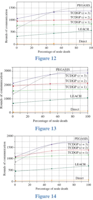
Nodes remaining alive network: We will show the distribution of nodes still functioning after several rounds. In the next Section we will also compare when each protocol reaches HND. The sink is located at (50, 300) and the number of cluster heads, c, ranges from 1 to 3. There are 100 nodes distributed in a 100 x 100 sensor field and the initial energy is determined to be 0.5J per node. It can clearly be seen in Fig. 9 that c = 1 has better performance than c = 2 or c = 3 at FND, HND, and LND From this we can find the threshold mechanism so that the node power is utilized uniformly. It can clearly be seen in Fig. 10 that the proposed protocol has a better number of rounds than other related methods at FND. We put the sink further away than in the previous scenario (at (50, 400)) as shown in Figs. 11-12 and found that the further away the sink is, the better the CDG. If the sink is far away from the sensor field, we can supply more network lifetime to gather sensed data. We changed the initial energy to compare the difference in related protocols and ours. The sink is located at (50, 300) and the number of cluster heads c, ranges from 1 to 3. There are 100 nodes distributed in a 100 x100 sensor field. The initial energies are 0.25J, 0.5J, and 1J, respectively. (Figs. 13-15,respectively). Because our threshold mechanism works regularly, the CDG can extend the whole network lifetime while ensuring the network integrity. When the initial energy is equal to 0.25 J and c = 3, the power is not enough to reveal the ability of our mechanism. Thus, the more initial power nodes, the better the performance it will be. Direct transmission is the same because the nodes in it are independent We changed the network density to compare related protocol to ours. The sink is located at (50, 300). The Number of cluster heads, c, ranges from 1 to 3. There are many nodes distributed in a 100 x 100 sensor field. The initial energy is 0.5J per node. We put 50, 100, and 200 nodes in the sensor field (Figs. 13-15, respectively). It can be seen that for the TGDGP with c = 1 we have the highest rounds of communication. When the network density is highest we also observe good performance. The results for the CDG with c = 1, 2, 3 are very similar.. we recorded the situation at several percentages of node death in the CDG. The sink is located at (50, 300). The Number of cluster heads, c, is equal to 3. There are 100 nodes distributed in a 100 x100 sensor field. The initial energy is 0.5J per nodes. It can be seen that the nodes in the CDG were uniformly dead. At the 50% dead point it can be seen that the distribution of dead nodes for direct transmission and PEGASIS is similar. This is due to the death probability of the two protocols being the same, in that the farther nodes will die first. In the LEACH protocol, cluster heads are selected according to the remaining power and node death distribution is similar to the proposed protocol.

(4)

Figure 6

Figure 7

Figure 8

Figure 9

Figure 10

Figure 11

Figure 12

Figure 13

Figure 14

1. Conclusion & Future work

The CDG has several advantages in WSNs for data gathering. Time to first node death is longer than in the protocols compared by about 14%. We can maintain the WSN integrity until FND (first node death). When the sink is far away from the sensor field, our CDG has the most data gathering rounds. We can then uniformly obtain results from dead nodes in WSNs at each percent of node death. We compared the dead node topology with other related protocols and found that only the LEACH is similar to ours. The other protocols demonstrate non-uniform node death, which results in a lack of sensor nodes in specific zones. The threshold mechanism plays an important role in the CDG. It protects the root node from a slow death because each node has a chance to be the root. The proposed mechanism is superior to the compared protocols; however the performance could be improved if a common equation for the parameters, t and a in the threshold mechanism, could be determined.

References

[1] Akkaya, K., and Younis, M., 2005, “A Survey on Routing Protocols for Wireless Sensor Networks,” Elsevier Ad Hoc Networks Journal, Vol. 3, No. 3, pp. 325-349.

[2] Akyildiz, L., Su, W., Sankarasubramaniam, Y., and Cayirci, E., 2002, “A Survey on Sensor Networks,” IEEE Communications Magazine, Vol. 40, No. 8, pp. 102-114. [3] Cheng, H., and Jia, X., 2005, “An Energy Efficient Routing Algorithm for Wireless Sensor Networks,” Wireless Communications, Networking and Mobile Computing, Vol. 2, pp. 905-910.

(5)

Applications, Vol. 2, pp. 452-460.

[5] Heinzelman, W., Chandrakasan, A., and Balakrishnan, H., 2000, “Energy-Efficient Communication Protocol for Wireless Micro-sensor Networks,” Proceedings of the 33rd annual Hawaii International Conference on System Sciences, Hawaii, USA, Vol. 2, pp. 1-10.

[6] Jiang, Q., and Manivannan, D., 2004, “Routing Protocols for Sensor Networks,” IEEE Consumer Communications and Networking Conference, Atlanta, Georgia USA, pp. 93-98. [7] Liang, Y., and Yu, H., 2005, “Energy Adaptive Cluster-Head Selection for Wireless Sensor Networks,” Parallel and Distributed Computing, Applications and Technologies, Dalian, China, pp. 634-638.

[8] Lindsey, S., Raghavendra, C. S., and Sivalingam, K. M., 2002, “Data Gathering Algorithms in Sensor Networks Using Energy Metrics,” IEEE Transactions On Parallel and Distributed Systems, Vol. 13, No. 9, pp. 924-935.

[9] Lindsey, S., and Raghavendra, C. S., 2002, “PEGASIS: Power-Efficient Gathering in Sensor Information Systems,” IEEE Aerospace Conference Proceedings, Vol. 3, pp. 1125-1130.

[10] Martirosyan, A., Boukerche, A., and Pazzi, R. W. N.,2008, “A Taxonomy of Cluster-Based Routing Protocols for Wireless Sensor Networks,” International Symposium on Parallel Architectures, Algorithms, and Networks, Sydney, Australia, pp. 247-253.

[11] Min, R., Bhardwaj, M., Cho, S., Sinha, A., Shih, E., Wang, A., and Chandrakasan, A. P., 2001, “Low Power Wireless Sensor Networks,”Proceedings of International Conference on VLSI Design, Bangalore, India, pp. 205.

[12] Muruganathan, S. D., Ma, D. C. F., Bhasin, R. I., and Fapojuwo, A. O., 2005, “A Centralized Energy- Efficient Routing Protocol for Wireless Sensor Networks,” IEEE, Communications Magazine, Vol. 43, No, 3, pp. 8-13.

[13] Rabaey, J. M., Ammer, M. J., da Silva, J. L., Patel, D., and Roundy, S., 2000, “PicoRadio Supports Ad Hoc Ultra-Low Power Wireless Networking, ”IEEE Computer, Vol. 33, No. 7, pp. 42-48.

[14]Satapathy, S. S., and Sarma, N., 2006, “TREEPSI: Tree based Energy Efficient Protocol for Sensor Information,” International Conference on Wireless and Optical Communications Networks, Bangalore, India, pp. 4.

[15] Sohrabi, K., Gao, J., Ailawadhi, V., and Pottie, G., 2000, “Protocols for Self Organization of A Wireless Sensor Network,”IEEE Personal Communications, Vol. 7, No. 5, pp. 16-27.