INTRODUCTION
Weigh-in-Motion (WIM) systems are de-signed for weighing vehicles driving across a measurement site. Because during measurements the vehicle has to come in physical contact with the components of the system, WIM systems al-ways use built-in sensors installed in road pave-ment. Each WIM system consists of force sensors placed in one, two or even several lines, perpen-dicular to the direction of traffic.
Literature reviews
The idea behind WIM systems is to measure the dynamic loads that the wheels of a moving vehicle exert on the road surface and, on this ba-sis, to estimate static wheel loads as well as gross vehicle weight. The accuracy of WIM measure-ments is determined by the measuring conditions, including:
• vehicle speed,
• quality of the road pavement in which the WIM system is installed [12],
• properties of the force sensors used [5, 10],
• calibration procedure and frequency of system calibration [1, 9, 8, 9, 11, 14],
• algorithm used for estimating static load and gross vehicle weight [13].
WIM systems are divided with respect to design and functionality criteria into two types: multi-sensor and classic mechanical systems. The more advanced and more complex Multi-Sensor WIM (MS WIM) systems [3, 4], are equipped with cameras, which make it possible to collect additional information regarding the fixed and variable parameters of road traffic. The fixed pa -rameters are characteristics such as vehicle class, registration number, number of axles, distances between individual axles, distances between extreme axles, and vehicle length. The variable parameters include time of vehicle arrival at the measurement point, vehicle speed, direction of movement, and the number of lane in which the vehicle was detected.
An MS-WIM system installed in a road lane al-lows automatic measurement of vehicle parameters, in particular axle loads and gross weight, without imposing significant speed limits. MS-WIM is a
GEOMETRIC OPTIMIZATION OF A BEAM DETECTOR FOR A WIM SYSTEM
Aleksander Nieoczym1, Kazimierz Drozd2, Andrzej Wójcik3
1 Lublin University of Technology, Ul. Nadbystrzycka 36, 20-618 Lublin, Poland, e-mail: [email protected]
2 Department of Materials Engineering, Lublin University of Technology, ul. Nadbystrzycka 36, 20-618 Lublin, Poland, e-mail: [email protected]
3 Departament of Machine Design and Mechatronics, Lublin University of Technology, ul. Nadbystrzycka 36, 20-618 Lublin, Poland, e-mail: [email protected])
Advances in Science and Technology Research Journal
Volume 12, Issue 3, September 2018, pages 233–241
DOI: 10.12913/22998624/97296 Review Article
ABSTRACT
Weigh-in-Motion (WIM) systems are designed for weighing vehicles driving across a measurement site. Because during measurements the vehicle has to come in physical contact with the components of the system, WIM systems always use built-in sensors installed in road pavement. Each WIM system consists of force sensors placed in one, two or even several lines, perpendicular to the direction of traffic. The idea behind WIM systems is to measure the dynamic loads that the wheels of a moving vehicle exert on the road surface and, on this basis, to estimate static wheel loads as well as gross vehicle weight.
Keywords: FEM, BEAM, weigh-in-motion, deflection of the beam, fibre optic sensor Received: 2018.01.02
multi-configuration system based on inductive loop systems with an optionally installed axle detector and polymer or quartz force sensors. The force sensors are distributed evenly along the measuring area. Each pair of force sensors is sur-rounded by an inductive loop, thus creating a du-al-sensor WIM subsystem. Each such subsystem cooperates with its own signal conditioning sys-tem, an a/d converter and a processor system that controls the acquisition of measurement signals, their pre-processing and transmission to the host system. The system is designed for measuring and determining traffic characteristics such as traffic density, vehicle flow, lane occupancy, average speed, and time distances between vehicles [2].
Mechanical WIM systems use piezoelectric and strain gauge sensors as vehicle-load-convert-ing elements. Piezoelectric sensors are mount-ed directly on a metal plate or beam (“bending plate”), which is subjected to vehicle axle loads. Axle loads and vehicle weights can also be mea-sured using detectors that have the form of a platform supported on mechanical elements (col-umns, beams), the so-called ‘load cells’, which are equipped with strain gauges for measuring deflection of the cells. The main advantage of load cells is their high measuring accuracy. They reach an accuracy of 2% during static measure-ments. The detectors used in dynamic conditions achieve an accuracy of ± 10% for gross weight measurements and approx. ± 15% for single-axle load measurements. Often, strain gauge scales are used as low-speed scales (vehicle speed up to 6 km/h); they have an accuracy similar to stationary weights. The nominal weighing capacity of this type of scales is up to 20 tons/axle. [15, 16]
Purpose of scientific and research works The WIM measuring systems described above are used as dynamic in-motion scales designed to monitor the weight of vehicles with a maximum permissible gross weight in the range from 3,500 kg to 36,000 kg. However, apart from weighing vehicles, it is often also necessary to simultane-ously analyse what types of vehicles (by number of wheels, e.g. two-wheelers, four wheelers, etc.) are participating in traffic. This type of analysis involves not only the measurement of vehicle weight but also qualitative detection. Such data are mainly collected and analysed in urban traffic, in which information on traffic volume, lane oc -cupancy or the number of vehicles waiting to
en-ter an inen-tersection are important from the point of view of ensuring continuous, smooth traffic flow. Defined in this way, the task of a WIM system is to measure the weight of vehicles moving on a road and to detect whether they are motorcycles, passenger cars, heavy goods vehicles, or other. Systems with inductive loops, commonly used in cities, enable the collection of traffic volume data, but they do not allow measurement of ve-hicle weight within the range given above (3,500 kg to 36,000 kg).
This article presents a design of a WIM sys-tem in which the detector is a beam with Bragg grating optical fibre sensors glued on it. Fibre Bragg gratings (FBG) are wavelength shift sen-sors, in which the wavelength of light shifts under the influence of the parameter measured.
A fibre optic sensor was used because it offers an array of advantages:
• high sensitivity to vertical forces (about 10% change in light intensity at loads exerted by an average-sized passenger vehicle),
• measurement of constant loads and loads vari-able in time,
• robustness to electromagnetic interference – systems with FBG sensors can be installed in the vicinity of high voltage power lines or rail-way, tram and trolleybus electric traction,
• high mechanical strength (long service life), resistance to corrosion, reliability and repeat-ability of measurements,
• it can be used on stations that do not have an electric power supply; the signal from the sen-sor can be sent through a fibre-optic cable at a distance of up to 2 km from the measuring point.
CALCULATION METHODOLOGY
Design of the beam detectorThe system was designed to detect the pres-ence and measure the weight of various vehicles ranging from motorcycles (single-truck vehicles) to trucks. The extreme values of permissible vehi-cle weight were assumed to be 250 kg and 10,000 kg. It was assumed that in a two-wheeled vehicle, the tyre force was 1000 N. A single axle of a truck with a gross vehicle weight m = 10,000 kg exerts a force of 60000 N.
Advances in Science and Technology Research Journal Vol. 12 (3), 2018
must not exceed εmax = 0.003 (0.3%), with the minimum value εmin = 0.000015 (0.0015%). Max-imum elongation of the sensor u = 0.045 mm.
The following design restrictions were de-fined for the beam:
• Stresses in the beam caused by the weight of a heavy goods vehicle may not exceed the per-missible stresses.
• The maximum relative elongation of the beam at the sensor mounting site caused by the weight of the car may not cause the maxi-mum relative elongation of the sensor to be exceeded.
• The measuring system must be able to detect the presence and measure the weight of a mo-torcycle in motion at any point along the width of the lane.
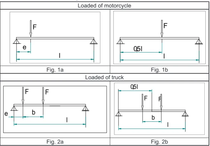
Based on the above assumptions, four cases of loading of the beam were considered which were important from the point of view of beam strength and the possibility of registering defor-mations (Table 1). Case 2b is related to permis-sible beam stresses and the maximum elongation of the sensor. Case 1a is associated with the mini-mum beam deformations that a fibre optic sensor can register.
Analytical strength calculations of the beam In cases in which a beam is loaded with the weight of a motorcycle, the placement of the fibre optic sensors on the beam is important. They must be glued in regions of maximum beam deflection.
The crux of the problem, therefore, is to calculate the value of the bending moment generated in the beam under the influence of a single-track vehicle and then to calculate whether the relative defor-mation of the beam under the influence of this moment can be registered by a fibre optic sensor.
The bending moment determined in any sec-tion defined by the coordinate variable x (Fig. 1):
Table 1. Cases of beam loading
Loaded of motorcycle
e F
l 0,5 l
F
l
Fig. 1a Fig. 1b
Loaded of truck
e
F
l F
b
0,5 l
F
l F
b
Fig. 2a Fig. 2b
Fig. 1. Schematic of beam loaded with a double-track vehicle: x – variable defining the distance from the support to the centre of the wheel, F – motorcycle tyre force, c – point of application of the force (the centre of the wheel of the motorcycle), RA, RB –
reac-tions on the supports, l – length of the beam
Section I:
𝑀𝑀𝑔𝑔 =𝐹𝐹 𝑏𝑏𝑙𝑙 𝑥𝑥 0≤ 𝑥𝑥 ≤ 𝑎𝑎 (1)
𝑀𝑀𝑔𝑔 =𝐹𝐹 𝑏𝑏𝑙𝑙 𝑥𝑥 − 𝐹𝐹(𝑥𝑥 − 𝑎𝑎) 𝑎𝑎 ≤ 𝑥𝑥 ≤ 𝑙𝑙 (2)
𝐸𝐸𝐽𝐽𝑦𝑦𝑤𝑤𝐼𝐼′′=𝐹𝐹𝑏𝑏𝐹𝐹
𝑙𝑙 (3)
𝐸𝐸𝐽𝐽𝑦𝑦𝑤𝑤𝐼𝐼𝐼𝐼′′=𝐹𝐹𝑏𝑏𝐹𝐹𝑙𝑙 − 𝑃𝑃𝑥𝑥+𝑃𝑃𝑎𝑎 (4)
𝑤𝑤
𝑐𝑐= (𝑤𝑤
𝐼𝐼)
𝐹𝐹=𝑎𝑎= (𝑤𝑤
𝐼𝐼𝐼𝐼)
𝐹𝐹=𝑎𝑎=
−
𝑃𝑃𝑎𝑎 2𝑏𝑏23𝐸𝐸𝐽𝐽𝑦𝑦𝑙𝑙 (5)
𝑥𝑥𝐼𝐼 =√13(𝑙𝑙2− 𝑏𝑏2) (6)
𝑓𝑓
= |𝑤𝑤
𝑚𝑚𝑎𝑎𝐹𝐹| =𝐹𝐹𝑏𝑏(𝑙𝑙2−𝑏𝑏2) 3 29√3𝐸𝐸𝐽𝐽𝑦𝑦 𝑙𝑙
(7)
𝑥𝑥1→√3𝑙𝑙 (8)
Then: 𝑥𝑥1−2𝑙𝑙 ≈0,08𝑙𝑙 (9)
|𝑤𝑤𝑚𝑚𝑎𝑎𝐹𝐹− 𝑤𝑤𝐹𝐹=0,5𝑙𝑙| ≤2,5%|𝑤𝑤𝑚𝑚𝑎𝑎𝐹𝐹| (10)
(1)
Section II:𝑀𝑀𝑔𝑔=𝐹𝐹𝑙𝑙𝑏𝑏𝑥𝑥 0≤ 𝑥𝑥 ≤ 𝑎𝑎 (1) 𝑀𝑀𝑔𝑔 =𝐹𝐹𝑙𝑙𝑏𝑏𝑥𝑥 − 𝐹𝐹(𝑥𝑥 − 𝑎𝑎) 𝑎𝑎 ≤ 𝑥𝑥 ≤ 𝑙𝑙 (2)
𝐸𝐸𝐽𝐽𝑦𝑦𝑤𝑤𝐼𝐼′′=𝐹𝐹𝑏𝑏𝐹𝐹
𝑙𝑙 (3) 𝐸𝐸𝐽𝐽𝑦𝑦𝑤𝑤𝐼𝐼𝐼𝐼′′=𝐹𝐹𝑏𝑏𝐹𝐹𝑙𝑙 − 𝑃𝑃𝑥𝑥+𝑃𝑃𝑎𝑎 (4)
𝑤𝑤
𝑐𝑐= (
𝑤𝑤
𝐼𝐼)
𝐹𝐹=𝑎𝑎= (
𝑤𝑤
𝐼𝐼𝐼𝐼)
𝐹𝐹=𝑎𝑎=
−
𝑃𝑃𝑎𝑎2𝑏𝑏2
3𝐸𝐸𝐽𝐽𝑦𝑦𝑙𝑙 (5)
𝑥𝑥𝐼𝐼 =√13(𝑙𝑙2− 𝑏𝑏2) (6)
𝑓𝑓
= |
𝑤𝑤
𝑚𝑚𝑎𝑎𝐹𝐹| =
𝐹𝐹𝑏𝑏(𝑙𝑙2−𝑏𝑏2)3 2
9√3𝐸𝐸𝐽𝐽𝑦𝑦𝑙𝑙
(7)
𝑥𝑥1 →√3𝑙𝑙 (8)
Then: 𝑥𝑥1−2𝑙𝑙 ≈0,08𝑙𝑙 (9)
|𝑤𝑤𝑚𝑚𝑎𝑎𝐹𝐹− 𝑤𝑤𝐹𝐹=0,5𝑙𝑙| ≤2,5%|𝑤𝑤𝑚𝑚𝑎𝑎𝐹𝐹| (10) (2)
Advances in Science and Technology Research Journal𝑙𝑙 Vol. 12 (3), 2018
𝑀𝑀𝑔𝑔=𝐹𝐹𝑙𝑙𝑏𝑏𝑥𝑥 − 𝐹𝐹(𝑥𝑥 − 𝑎𝑎) 𝑎𝑎 ≤ 𝑥𝑥 ≤ 𝑙𝑙 (2)
𝐸𝐸𝐽𝐽𝑦𝑦𝑤𝑤𝐼𝐼′′ =𝐹𝐹𝑏𝑏𝐹𝐹 𝑙𝑙 (3)
𝐸𝐸𝐽𝐽𝑦𝑦𝑤𝑤𝐼𝐼𝐼𝐼′′=𝐹𝐹𝑏𝑏𝐹𝐹𝑙𝑙 − 𝑃𝑃𝑥𝑥+𝑃𝑃𝑎𝑎 (4)
𝑤𝑤
𝑐𝑐= (
𝑤𝑤
𝐼𝐼)
𝐹𝐹=𝑎𝑎= (
𝑤𝑤
𝐼𝐼𝐼𝐼)
𝐹𝐹=𝑎𝑎=
−
𝑃𝑃𝑎𝑎 2𝑏𝑏2 3𝐸𝐸𝐽𝐽𝑦𝑦𝑙𝑙 (5)𝑥𝑥𝐼𝐼=√13(𝑙𝑙2− 𝑏𝑏2) (6)
𝑓𝑓
= |
𝑤𝑤𝑚𝑚𝑎𝑎𝐹𝐹
| =
𝐹𝐹𝑏𝑏(𝑙𝑙2−𝑏𝑏2) 3 2 9√3𝐸𝐸𝐽𝐽𝑦𝑦𝑙𝑙(7)
𝑥𝑥1 →√3𝑙𝑙 (8)
Then: 𝑥𝑥1−2𝑙𝑙 ≈0,08𝑙𝑙 (9)
|𝑤𝑤𝑚𝑚𝑎𝑎𝐹𝐹− 𝑤𝑤𝐹𝐹=0,5𝑙𝑙| ≤2,5%|𝑤𝑤𝑚𝑚𝑎𝑎𝐹𝐹| (10)
(3) 𝑀𝑀𝑔𝑔 =𝐹𝐹𝑙𝑙𝑏𝑏𝑥𝑥 − 𝐹𝐹(𝑥𝑥 − 𝑎𝑎) 𝑎𝑎 ≤ 𝑥𝑥 ≤ 𝑙𝑙 (2)
𝐸𝐸𝐽𝐽𝑦𝑦𝑤𝑤𝐼𝐼′′=𝐹𝐹𝑏𝑏𝐹𝐹 𝑙𝑙 (3)
𝐸𝐸𝐽𝐽𝑦𝑦𝑤𝑤𝐼𝐼𝐼𝐼′′ =𝐹𝐹𝑏𝑏𝐹𝐹 𝑙𝑙 − 𝑃𝑃𝑥𝑥+𝑃𝑃𝑎𝑎 (4)
𝑤𝑤
𝑐𝑐= (
𝑤𝑤
𝐼𝐼)
𝐹𝐹=𝑎𝑎= (
𝑤𝑤
𝐼𝐼𝐼𝐼)
𝐹𝐹=𝑎𝑎=
−
𝑃𝑃𝑎𝑎 2𝑏𝑏2 3𝐸𝐸𝐽𝐽𝑦𝑦𝑙𝑙 (5)𝑥𝑥𝐼𝐼 =√13(𝑙𝑙2− 𝑏𝑏2) (6)
𝑓𝑓
= |
𝑤𝑤𝑚𝑚𝑎𝑎𝐹𝐹
| =
𝐹𝐹𝑏𝑏(𝑙𝑙2−𝑏𝑏2) 3 2 9√3𝐸𝐸𝐽𝐽𝑦𝑦𝑙𝑙(7)
𝑥𝑥1→√3𝑙𝑙 (8)
Then: 𝑥𝑥1−2𝑙𝑙 ≈0,08𝑙𝑙 (9)
|𝑤𝑤𝑚𝑚𝑎𝑎𝐹𝐹− 𝑤𝑤𝐹𝐹=0,5𝑙𝑙| ≤2,5%|𝑤𝑤𝑚𝑚𝑎𝑎𝐹𝐹| (10)
(4) By using integration, we get the following solution: 𝑀𝑀𝑔𝑔 =𝐹𝐹 𝑏𝑏𝑙𝑙 𝑥𝑥 0≤ 𝑥𝑥 ≤ 𝑎𝑎 (1)
𝑀𝑀𝑔𝑔 =𝐹𝐹 𝑏𝑏𝑙𝑙 𝑥𝑥 − 𝐹𝐹(𝑥𝑥 − 𝑎𝑎) 𝑎𝑎 ≤ 𝑥𝑥 ≤ 𝑙𝑙 (2)
𝐸𝐸𝐽𝐽𝑦𝑦𝑤𝑤𝐼𝐼′′=𝐹𝐹𝑏𝑏𝐹𝐹 𝑙𝑙 (3)
𝐸𝐸𝐽𝐽𝑦𝑦𝑤𝑤𝐼𝐼𝐼𝐼′′=𝐹𝐹𝑏𝑏𝐹𝐹 𝑙𝑙 − 𝑃𝑃𝑥𝑥+𝑃𝑃𝑎𝑎 (4)
𝑤𝑤
𝑐𝑐= (𝑤𝑤𝐼𝐼)𝐹𝐹=𝑎𝑎
= (𝑤𝑤𝐼𝐼𝐼𝐼)𝐹𝐹=𝑎𝑎
=
−
𝑃𝑃𝑎𝑎 2𝑏𝑏2 3𝐸𝐸𝐽𝐽𝑦𝑦𝑙𝑙 (5)𝑥𝑥𝐼𝐼 =√13(𝑙𝑙2− 𝑏𝑏2) (6)
𝑓𝑓
= |𝑤𝑤
𝑚𝑚𝑎𝑎𝐹𝐹| =𝐹𝐹𝑏𝑏(𝑙𝑙2−𝑏𝑏2) 3 2 9√3𝐸𝐸𝐽𝐽𝑦𝑦 𝑙𝑙(7)
𝑥𝑥1→√3𝑙𝑙 (8)
Then: 𝑥𝑥1−2𝑙𝑙 ≈0,08𝑙𝑙 (9)
|𝑤𝑤𝑚𝑚𝑎𝑎𝐹𝐹− 𝑤𝑤𝐹𝐹=0,5𝑙𝑙| ≤2,5%|𝑤𝑤𝑚𝑚𝑎𝑎𝐹𝐹| (10)
(5) Maximum deflection f = |wmax|: When a> 0.5 l then wmax is in section I and the cor-responding coordinate has the value: 𝑀𝑀𝑔𝑔 =𝐹𝐹𝑙𝑙𝑏𝑏𝑥𝑥 0≤ 𝑥𝑥 ≤ 𝑎𝑎 (1)
𝑀𝑀𝑔𝑔=𝐹𝐹𝑙𝑙𝑏𝑏𝑥𝑥 − 𝐹𝐹(𝑥𝑥 − 𝑎𝑎) 𝑎𝑎 ≤ 𝑥𝑥 ≤ 𝑙𝑙 (2)
𝐸𝐸𝐽𝐽𝑦𝑦𝑤𝑤𝐼𝐼′′ =𝐹𝐹𝑏𝑏𝐹𝐹𝑙𝑙 (3)
𝐸𝐸𝐽𝐽𝑦𝑦𝑤𝑤𝐼𝐼𝐼𝐼′′=𝐹𝐹𝑏𝑏𝐹𝐹𝑙𝑙 − 𝑃𝑃𝑥𝑥+𝑃𝑃𝑎𝑎 (4)
𝑤𝑤
𝑐𝑐= (
𝑤𝑤
𝐼𝐼)
𝐹𝐹=𝑎𝑎= (
𝑤𝑤
𝐼𝐼𝐼𝐼)
𝐹𝐹=𝑎𝑎=
−
𝑃𝑃𝑎𝑎 2𝑏𝑏2 3𝐸𝐸𝐽𝐽𝑦𝑦𝑙𝑙 (5)𝑥𝑥𝐼𝐼=√13(𝑙𝑙2− 𝑏𝑏2) (6)
𝑓𝑓
= |
𝑤𝑤
𝑚𝑚𝑎𝑎𝐹𝐹| =
𝐹𝐹𝑏𝑏(𝑙𝑙2−𝑏𝑏2) 3 2 9√3𝐸𝐸𝐽𝐽𝑦𝑦𝑙𝑙(7)
𝑥𝑥1 →√3𝑙𝑙 (8)
Then: 𝑥𝑥1−2𝑙𝑙 ≈0,08𝑙𝑙 (9)
|𝑤𝑤𝑚𝑚𝑎𝑎𝐹𝐹− 𝑤𝑤𝐹𝐹=0,5𝑙𝑙| ≤2,5%|𝑤𝑤𝑚𝑚𝑎𝑎𝐹𝐹| (10)
(6) And maximum deflection is: 𝑀𝑀𝑔𝑔 =𝐹𝐹𝑙𝑙𝑏𝑏𝑥𝑥 0≤ 𝑥𝑥 ≤ 𝑎𝑎 (1)
𝑀𝑀𝑔𝑔 =𝐹𝐹𝑙𝑙𝑏𝑏𝑥𝑥 − 𝐹𝐹(𝑥𝑥 − 𝑎𝑎) 𝑎𝑎 ≤ 𝑥𝑥 ≤ 𝑙𝑙 (2)
𝐸𝐸𝐽𝐽𝑦𝑦𝑤𝑤𝐼𝐼′′=𝐹𝐹𝑏𝑏𝐹𝐹𝑙𝑙 (3)
𝐸𝐸𝐽𝐽𝑦𝑦𝑤𝑤𝐼𝐼𝐼𝐼′′ =𝐹𝐹𝑏𝑏𝐹𝐹 𝑙𝑙 − 𝑃𝑃𝑥𝑥+𝑃𝑃𝑎𝑎 (4)
𝑤𝑤
𝑐𝑐= (
𝑤𝑤𝐼𝐼
)
𝐹𝐹=𝑎𝑎= (
𝑤𝑤𝐼𝐼𝐼𝐼
)
𝐹𝐹=𝑎𝑎=
−
𝑃𝑃𝑎𝑎 2𝑏𝑏2 3𝐸𝐸𝐽𝐽𝑦𝑦𝑙𝑙 (5)𝑥𝑥𝐼𝐼 =√13(𝑙𝑙2− 𝑏𝑏2) (6)
𝑓𝑓
= |
𝑤𝑤
𝑚𝑚𝑎𝑎𝐹𝐹| =
𝐹𝐹𝑏𝑏(𝑙𝑙2−𝑏𝑏2) 3 2 9√3𝐸𝐸𝐽𝐽𝑦𝑦𝑙𝑙(7)
𝑥𝑥1→√3𝑙𝑙 (8)
Then: 𝑥𝑥1−2𝑙𝑙 ≈0,08𝑙𝑙 (9)
|𝑤𝑤𝑚𝑚𝑎𝑎𝐹𝐹− 𝑤𝑤𝐹𝐹=0,5𝑙𝑙| ≤2,5%|𝑤𝑤𝑚𝑚𝑎𝑎𝐹𝐹| (10)
(7) The x coordinate described by formula (6) does not deviate much from the value of 0.5l. Even when b → 0: 𝑀𝑀𝑔𝑔 =𝐹𝐹𝑙𝑙𝑏𝑏𝑥𝑥 0≤ 𝑥𝑥 ≤ 𝑎𝑎 (1)
𝑀𝑀𝑔𝑔 =𝐹𝐹𝑙𝑙𝑏𝑏𝑥𝑥 − 𝐹𝐹(𝑥𝑥 − 𝑎𝑎) 𝑎𝑎 ≤ 𝑥𝑥 ≤ 𝑙𝑙 (2)
𝐸𝐸𝐽𝐽𝑦𝑦𝑤𝑤𝐼𝐼′′=𝐹𝐹𝑏𝑏𝐹𝐹𝑙𝑙 (3)
𝐸𝐸𝐽𝐽𝑦𝑦𝑤𝑤𝐼𝐼𝐼𝐼′′=𝐹𝐹𝑏𝑏𝐹𝐹 𝑙𝑙 − 𝑃𝑃𝑥𝑥+𝑃𝑃𝑎𝑎 (4)
𝑤𝑤
𝑐𝑐= (
𝑤𝑤𝐼𝐼
)
𝐹𝐹=𝑎𝑎= (
𝑤𝑤𝐼𝐼𝐼𝐼
)
𝐹𝐹=𝑎𝑎=
−
𝑃𝑃𝑎𝑎 2𝑏𝑏2 3𝐸𝐸𝐽𝐽𝑦𝑦𝑙𝑙 (5)𝑥𝑥𝐼𝐼 =√13(𝑙𝑙2− 𝑏𝑏2) (6)
𝑓𝑓
= |
𝑤𝑤
𝑚𝑚𝑎𝑎𝐹𝐹| =
𝐹𝐹𝑏𝑏(𝑙𝑙2−𝑏𝑏2) 3 2 9√3𝐸𝐸𝐽𝐽𝑦𝑦𝑙𝑙(7)
𝑥𝑥1→√3𝑙𝑙 (8)
Then: 𝑥𝑥1−2𝑙𝑙 ≈0,08𝑙𝑙 (9)
|𝑤𝑤𝑚𝑚𝑎𝑎𝐹𝐹− 𝑤𝑤𝐹𝐹=0,5𝑙𝑙| ≤2,5%|𝑤𝑤𝑚𝑚𝑎𝑎𝐹𝐹| (10)
(8) Then: 𝑀𝑀𝑔𝑔 =𝐹𝐹𝑙𝑙𝑏𝑏𝑥𝑥 0≤ 𝑥𝑥 ≤ 𝑎𝑎 (1)
𝑀𝑀𝑔𝑔 =𝐹𝐹𝑙𝑙𝑏𝑏𝑥𝑥 − 𝐹𝐹(𝑥𝑥 − 𝑎𝑎) 𝑎𝑎 ≤ 𝑥𝑥 ≤ 𝑙𝑙 (2)
𝐸𝐸𝐽𝐽𝑦𝑦𝑤𝑤𝐼𝐼′′=𝐹𝐹𝑏𝑏𝐹𝐹𝑙𝑙 (3)
𝐸𝐸𝐽𝐽𝑦𝑦𝑤𝑤𝐼𝐼𝐼𝐼′′=𝐹𝐹𝑏𝑏𝐹𝐹𝑙𝑙 − 𝑃𝑃𝑥𝑥+𝑃𝑃𝑎𝑎 (4)
𝑤𝑤
𝑐𝑐= (
𝑤𝑤
𝐼𝐼)
𝐹𝐹=𝑎𝑎= (
𝑤𝑤
𝐼𝐼𝐼𝐼)
𝐹𝐹=𝑎𝑎=
−
𝑃𝑃𝑎𝑎 2𝑏𝑏2 3𝐸𝐸𝐽𝐽𝑦𝑦𝑙𝑙 (5)𝑥𝑥𝐼𝐼 =√13(𝑙𝑙2− 𝑏𝑏2) (6)
𝑓𝑓
= |
𝑤𝑤
𝑚𝑚𝑎𝑎𝐹𝐹| =
𝐹𝐹𝑏𝑏(𝑙𝑙2−𝑏𝑏2) 3 2 9√3𝐸𝐸𝐽𝐽𝑦𝑦𝑙𝑙(7)
𝑥𝑥1→√3𝑙𝑙 (8)
Then: 𝑥𝑥1−2𝑙𝑙 ≈0,08𝑙𝑙 (9)
|𝑤𝑤𝑚𝑚𝑎𝑎𝐹𝐹− 𝑤𝑤𝐹𝐹=0,5𝑙𝑙| ≤2,5%|𝑤𝑤𝑚𝑚𝑎𝑎𝐹𝐹| (10)
(9) This makes the difference: wmax – wx=0,5l small, and in the limit case, when b → 0 then: 𝑀𝑀𝑔𝑔 =𝐹𝐹 𝑏𝑏𝑙𝑙 𝑥𝑥 0≤ 𝑥𝑥 ≤ 𝑎𝑎 (1)
𝑀𝑀𝑔𝑔=𝐹𝐹 𝑏𝑏𝑙𝑙 𝑥𝑥 − 𝐹𝐹(𝑥𝑥 − 𝑎𝑎) 𝑎𝑎 ≤ 𝑥𝑥 ≤ 𝑙𝑙 (2)
𝐸𝐸𝐽𝐽𝑦𝑦𝑤𝑤𝐼𝐼′′=𝐹𝐹𝑏𝑏𝐹𝐹𝑙𝑙 (3)
𝐸𝐸𝐽𝐽𝑦𝑦𝑤𝑤𝐼𝐼𝐼𝐼′′=𝐹𝐹𝑏𝑏𝐹𝐹𝑙𝑙 − 𝑃𝑃𝑥𝑥+𝑃𝑃𝑎𝑎 (4)
𝑤𝑤
𝑐𝑐= (𝑤𝑤
𝐼𝐼)
𝐹𝐹=𝑎𝑎= (𝑤𝑤
𝐼𝐼𝐼𝐼)
𝐹𝐹=𝑎𝑎=
−
𝑃𝑃𝑎𝑎 2𝑏𝑏2 3𝐸𝐸𝐽𝐽𝑦𝑦𝑙𝑙 (5)𝑥𝑥𝐼𝐼=√13(𝑙𝑙2− 𝑏𝑏2) (6)
𝑓𝑓
= |𝑤𝑤
𝑚𝑚𝑎𝑎𝐹𝐹| =
𝐹𝐹𝑏𝑏(𝑙𝑙2−𝑏𝑏2) 3 2 9√3𝐸𝐸𝐽𝐽𝑦𝑦 𝑙𝑙(7)
𝑥𝑥1 →√3𝑙𝑙 (8)
Then: 𝑥𝑥1−2𝑙𝑙 ≈0,08𝑙𝑙 (9)
|𝑤𝑤𝑚𝑚𝑎𝑎𝐹𝐹− 𝑤𝑤𝐹𝐹=0,5𝑙𝑙| ≤2,5%|𝑤𝑤𝑚𝑚𝑎𝑎𝐹𝐹| (10) (10)
Calculation results
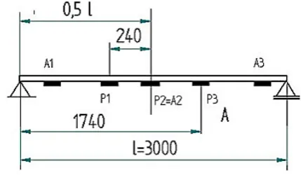
Whether the beam can be used as a signal transmitter for optical fibre sensors is determined by its deflection under the influence of a passing single-track (low weight) vehicle Deflection of the beam, uniquely defined by maximum deflection f, is associated with its deflection line. Maximum de -flection calculated with the formulas (8) and (9) in -dicates that the fibre optic sensors should be placed symmetrically at a distance of 240 mm from the centre of the beam at points P1, P2, and P3 (Fig. 2).
FEM strength calculations using Abaqus soft-ware were conducted . The results of modeling – points P1, P2, P3 are shown in Table 2–5.
Fig. 2. Location of sensors: P1, P2, P3 – placement points for fibre optic sensors determined in beam deflec -tion calcula-tions, A1, A2, A3 – sensor placement points resulting from geometric optimization of the beam
Table 2. Results of modelling FEM , case 1a (Table 1)
Point Stresses in the direction of the beam axis [N/mm2] Deflection of the beam[mm] Deformation [xE-5]
P1 1.31 0.135 0.62
P2 1.09 0.131 0.52
P3 0.95 0.121 0.45
Table 3. Results of modelling FEM, case 1b (Table 1)
Point Stresses in the direction of the beam axis [N/mm2] Deflection of the beam[mm] Deformation [xE-5]
P1 5.70 0.51 2.69
P2 6.29 0.52 2.95
P3 5.70 0.51 2.69
Table 4. Results of modelling FEM, case 2a (Table 1)
Point Stresses in the direction of the beam axis [N/mm2] Deflection of the beam[mm] Deformation [xE-5]
P1 126.26 13.77 59.82
P2 136.50 14.34 65.00
Advances in Science and Technology Research Journal Vol. 12 (3), 2018
Results on the correctness of modelling:
• Maximum stress produced in the beam by a vehicle’s weight does not exceed permissible stress.
• Deflection of the beam under the weight of a motorcycle is too small to be registered by a fibre optic sensor.
Optimization of the beam shape
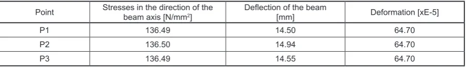
Due to the fact that the beam was character-ized by excessive stiffness which made it impos -sible to identify a single-track vehicle, the shape of the beam was optimized. The optimization in-volved introduction of local changes in the cross-section of the existing beam. Longitudinal holes, 100 mm wide and 250 mm long, were made in the lower plane of the beam (Fig. 3). Two sensors were glued inside the beam along the longitudinal edge of the hole at a distance of 384 mm from the end of the beam, 20 mm from the edge of the hole – points A1 and A3. A third sensor was attached to the beam at its mid-length – point A2 (equiva-lent to point P2). The advantage of the change in the geometry of the beam is that the sensors and connecting cables inside the beam are protected Table 5. Results of modelling FEM, case 2b (Table 1)
Point Stresses in the direction of the beam axis [N/mm2] Deflection of the beam[mm] Deformation [xE-5]
P1 136.49 14.50 64.70
P2 136.50 14.94 64.70
P3 136.49 14.55 64.70
Fig. 3. Beam after the process of geometric optimization
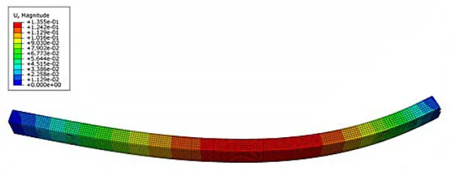
from damage. Tables 6–8 show the results of FEM strength analysis. The results of modeling are presented in Figures 4–15.
CONCLUSIONS
Applications for optimization of geometric beam detector with the use of CAD:
1. Parametric models describing the influence of vehicle tyre force depending on the location of
Table 6. Results of modelling FEM, beam with holes, case 1a (Table 1)
Point Stresses in the direction of the beam axis [N/mm2] Deflection of the beam[mm] Deformation [xE-5]
A1 3.90 0.079 1.83
P1 1.31 0.140 0.62
P2 = A2 1.09 0.135 0.52
P3 0.95 0.125 0.45
A3 0.62 0.047 0.29
Table 7. Results of modelling FEM, beam with holes, case 1b (Table 1)
Point Stresses in the direction of the beam axis [N/mm2] Deflection of the beam[mm] Deformation [xE-5]
A1 3.66 0.204 1.72
P1 5.70 0.52 2.70
P2 = A2 6.29 0.53 2.95
P3 5.70 0.52 2.70
Table 8. Results of modelling FEM, beam with holes, case 2a (Table 1)
Point Stresses in the direction of the beam axis [N/mm2] Deflection of the beam[mm] Deformation [xE-5]
A1 161.35 6.13 75.30
P1 125.63 9.92 59.82
P2 = A2 136.50 14.68 64.67
P3 147.24 14.11 70.09
A3 183.68 6.41 86.31
Table 9. Results of modelling FEM, beam with holes, case 2b (Table 1)
Point Stresses in the direction of the beam axis [N/mm2] Deflection of the beam[mm] Deformation [xE-5]
A1 187.46 6.30 87.53
P1 136.49 14.83 65.00
P2 = A2 136.49 15.27 65.00
P3 136.49 14.88 65.00
A3 186.90 6.53 87.26
Fig. 4. Reduced stresses, case 1a
Fig. 5. Deformation, case 1a
Advances in Science and Technology Research Journal Vol. 12 (3), 2018
Fig. 7. Reduced stresses, case 1a, beam after the pro-cess of geometric optimization
Fig. 8. Deformation, case 1a, beam after the process of geometric optimization
Fig. 9. Deflection, case 1a, beam after the process of geometric optimization
Fig. 10. Reduced stresses, case 2b
Fig. 11. Deformation, case 2b
Fig. 12. Deflection, case 2b
Fig. 14. Deformation, case 2b, beam after the process
of geometric optimization Fig. 15. Deflection, case 2b, beam after the process of geometric optimization
the wheel on the detector beam of a WIM sys-tem were developed and verified.
2. The fibre optic sensors were located on the beam so that they could register beam defor-mations produced by the weight of a single-track vehicle.
3. Parametric models were used to optimize the shape of the beam so that it could be used to measure the weight of vehicles within the per-missible total weight from 250 kg to 10,000 kg and to detect certain road traffic parameters. 4. The selected shape of the holes reducing the
stiffness of the beam did not lead to exceed of the permissible stresses in any cross-section of the beam under the weight of the truck, the re-duced stresses have the value σzred = 187 MPa and do not exceed the yield point. The holes created increase the flexibility of the beam and enable registration of the weight and presence of the motorcycle. The beam deformation val-ue takes the valval-ue of ε = 1,83e-5 with the
mini-mum strain value possible to register by a fiber optic sensor equal to ε = 1.5 e-5
Conclusions regarding further model tests 5. The next research problem should be the
opti-mization of the shape of the beam supports in order to limit the deformation of the beam ends under the supports.
Applications regarding the use of a beam detector
6. The article presents the concept of construct-ing a beam detector of the WMS system, which can be used as a replacement for Multi Sensor Weigh in Motion (MS-WIM) systems
7. The beam detector was based on a typical rect-angular beam into which optical fiber sensors were inserted. The total cost of carrying out the beam detector along with the data acquisition equipment and the installation cost is around USD 15,000. For comparison, identical costs of mechanical WIM detectors with quartz and tensometric sensors are respectively: 32000 USD and 61000 USD [16]
8. The presented beam detector has the ability to identify the occurrence of vehicles in the field of pressure on the ground from 1000 N to 60000 N. Increasing the sensitivity of the detector can be obtained by placing in the beam two addi-tional fiber optic sensors placed symmetrically between the sensors already installed.
9. Verification tests performed on the real beam detector, next to the beam deflection and de -formation measurements, should be directed at the selection of a filling gel with an inserted beam in the road lane. Selection of the gel should guarantee the stability of its physical and chemical parameters in changing atmo-spheric conditions.
REFERENCES
1. Burnos, P., et al. Accurate weighing of moving ve-hicles. Metrology and Measurement Systems. vol. 14 no. 4, 2007, 507–516.
Advances in Science and Technology Research Journal Vol. 12 (3), 2018
3. Cebon, D. Design of multiple-sensor weigh-in-mo-tion systems. Journal of Automobile Engineering, Proc. I. Mech. E., 204, 1990, 133 – 144.
4. Cebon, D., Winkler CB. Multiple-Sensor WIM: Theory and experiments, Transportation Research Record, TRB, 1311, 1991, 70 -78.
5. Cole, D.J., Cebon, D. Performance and application of a capacitive strip tire force sensor. 6th Interna-tional Conference on Road Traffic Monitoring and Control. IEE, London, 1992, 123-127.
6. Dolcemascolo V., Jacob B. Multiple sensor Weigh-In-Motion: Optimal Design and Experimental Study. Pre-proceedings of 2nd European Confer-ence of Weigh in Motion of Road Vehicles, Lisbon, 1998, 129-138,.
7. Gajda J. Statistical calibration of WIM systems. Scientific Series of Rzeszów Politechnic, Electro -technic, nr 27, 2004 (in Polish).
8. Gajda J., Burnos P. Self-calibration of the weigh-in-motion systems. Proceedings of XV Sympo-sium Modelling and Simulation of Measurement Systems. 2005 (in Polish).
9. Gajda, J., et al.,. Accuracy analysis of WIM sys-tems calibrated using pre-weighed vehicles meth-od. Metrology and Measurement Systems. vol. 14, no. 4, 2007, 517–527.
10. Hoose N., Kunz J., 1998. Implementation and tests of quartz crystal sensor WIM system. Proceedings of 2nd European Conference „Weigh in Motion of Road Vehicle”, Lisbon, 1998, 461-466.
11. Huhtala, M.,. Factors Affecting Calibration Effec -tiveness. Proceedings of the Final Symposium of the Project WAVE, Paris. 1999
12. Jacob B. Weigh-in Motion of Road Vehicle. Final Report of COST 323 action, ver. 3.0. 1999.
13. Mangeas, M., Glaser S., Dolcemascolo V. Neural networks estimation of truck static weights by fusing weight-in-motion data. Proc. of Eurofusion, 2000. 14. Stanczyk, D. New Calibration Procedure by Axle
Rank. Proceedings of the Final Symposium of the Project WAVE, Paris, 1999
15. http://www.traffic-1.pl