MHD UNSTEADY FLOW OF A WILLIAMSON NANOFLUID IN A VERTICAL POROUS SPACE WITH OSCILLATING WALL TEMPERATURE

* _{Corresponding author email: dr.ramamoorthymuthuraj@gmail.com}

MHD UNSTEADY FLOW OF A WILLIAMSON NANOFLUID IN A

VERTICAL POROUS SPACE WITH OSCILLATING WALL

TEMPERATURE

D. Lourdu Immaculate

a

_{, R. Muthuraj}

b, *

_,

_{Anant Kant Shukla}

c

_{and S. Srinivas}

d

a _{Research Scholar, Department of Mathematics, Bharathiar University, Coimbatore and Faculty in dept. of Mathematics, The American College,}

Madurai-625 002.

b _{Department of Mathematics, P.S.N.A. College of Engineering & Technology, Dindigul-624622, India.}

c _{Department of Mathematics, Amrita School of Engineering, Coimbatore, Amrita Vishwa Vidyapeetham, Amrita University, India} d _{Fluid Dynamics Division, School of Advanced Sciences, VIT University, Vellore – 632 014, India.}

ABTRACT

This article aims to examine the MHD unsteady flow of Williamson nanofluid in a vertical channel filled with a porous material and oscillating wall temperature. The modeling of this problem is transformed to ordinary differential equations by collecting the non-periodic and periodic terms and then series solutions are obtained by using a powerful method known as the homotopy analysis method (HAM). The influence of involved parameters on heat and mass transfer characteristics of the fluid flow is computed and presented graphically. Further, variations on volume flow rate, coefficient of skin friction, heat transfer rate and mass transfer rate are also discussed through tables. The study reveals that with increasing thermophoresis parameter, the fluid velocity decrease significantly however an enhancement in temperature distribution is noticed. With an increase in Prandtl number lead to enhance fluid temperature whereas it lead to decrease the fluid concentration considerably.

Keywords: Unsteady flow, Porous medium, Williamson nanofluid, Vertical channel, HAM.

1. INTRODUCTION

Nanofluid is a fluid containing small particles, called nanoparticles. These fluids are engineered colloidal suspensions of nanoparticles in a base fluid. Previous studies indicate that an enormous enhancement in the emission intensity, quantum yield, and lifetime of the molecular rectangles has been observed when the solvent medium is changed from organic to aqueous (Manimaran et al., 2002; Manimaran et al., 2003). In particular, Alkoxy-bridged rhenium (I) rectangles

3 2 3 2

[{(CO) Re(µ −OR) Re(CO) } (µ −bpy) ]₂ (1,R =C H ; 2, R _{4 9} =C H ; 3, R =_{8 17} C H ; bpy=4, 4' -bipyridine) comprising long alkyl _{12 25} chains form optically transparent aggregates and exhibit luminescence enhancement in the presence of water. Addition of water favors the aggregation of Re(I) molecular rectangle resulting in the luminescence enhancement, and this phenomenon has been traced out using light scattering techniques. Generally, the nanoparticles used in nanofluids are typically made of metals, oxides, carbides, or carbon nanotubes and the base fluids used are usually water, ethylene glycol and oil. Moreover, the study of nanofluid is of growing interest for the observation of enhanced thermal conductivity which may throw light on the urgent cooling problems in engineering, for instance, the cooling of integrated circuits and micro-electromechanical systems (See Lee et al., 1999, Manimaran et al., 2002; Manimaran et al., 2003; Xuan and Li, 2003; Buongiorno, 2006; Thanasekaran, et al., 2007, Marga et al., 2005; Kakac, Pramuanjaroenkij, 2009). Vajravelu et al. (2011) presented the detailed analysis of convective heat transfer in the flow of viscous Ag–

water and Cu–water nanofluids over a stretching surface. In reality most liquids are non-newtonian in nature, which are abundantly used in many industrial and engineering applications. In view of this, Niu et al. (2012) have theoretically investigated the slip-flow and heat transfer of a non-newtonian nanofluid in a microtube in which the power-law rheology is adopted to describe the non-newtonian characteristics of the flow. Xu et al. (2013) have analyzed the mixed convection flow of a nanofluid in a vertical channel with the Buongiorno mathematical model. Noreen et al. (2013) have discussed the mixed convection flow of nanofluid in the presence of an inclined magnetic field. Akbar et al. (2013) have examined the numerical study of Williamson nanofluid flow in an asymmetric channel. Hina et al. (2014) have studied the peristaltic transport of nanofluids in a curved channel with the effects of Brownian motion and thermophoretic diffusion of nanoparticles using long wavelength and low Reynolds number assumptions. Srinivas et al. (2014) have presented the flow and thermal analysis of nanofluid in the wavy channel using CFD package assuming single phase approach. The theoretical investigation of MHD Williamson nanofluid in a tapered asymmetric channel under the action of a thermal radiation parameter with peristalsis was studied by Kothandapani and Prakash (2015) and the authors have indicated that such analysis may serve for the intrauterine fluid motion in a sagittal cross-section of the uterus under cancer therapy and drug analysis. More recently, Shehzad et al. (2015) have investigated the two-dimensional magnetohydrodynamic (MHD) boundary layer flow of nanofluid in the presence of an applied magnetic field with Brownian motion and thermophoresis effects. Mixed convection flow through a channel has be en extensively studied

Frontiers in Heat and Mass Transfer

because of its occurrence in many practical applications such as the cooling of modern electronic systems, heat exchangers, solar energy collection, chemical processing equipments, transport of heated or cooled fluids, etc. The analysis of heat and mass transfer in porous media has been the important subject due to its practical applications such as packed-bed catalytic reactor, geothermal reservoirs, solid-matrix heat exchangers, chemical catalytic reactors, high performance insulation for buildings, drying of porous solids, thermal insulation, and petroleum resources etc (Cimpean et al., 2009; Srinivas and Muthuraj,2010; Abdul Hakeem et al., 2014; Freidoonimehr et al., 2015; Srinivasacharya and Swamy Reddy, 2015). Most of the previous studies discussed the mixed convection problems in porous media based on the model of Darcy's law that neglects important effects such as boundary and inertia effects. The pioneering work on the boundary and inertia effects of porous media on convective flow and heat transfer was analyzed by Vafai and Tien (1981). These models have been applied for simulating more generalized situations such as flow through packed and fluidized beds and liquid metal flow through dendritic structures in alloy casting(Vafai and Tien, 1981; Kou and Lu, 1993, Nithiarasu et al., 1997; Cimpean et al., 2009; Srinivas and Muthuraj,2010; Abdul Hakeem et al., 2014; Freidoonimehr et al., 2015; Srinivasacharya and Swamy Reddy, 2015). Cimpean et al. (2009) examined a fully developed mixed convection flow between inclined parallel flat plates filled with a porous medium with constant flow rate and uniform heat flux. Further, convective flows with applying uniform magnetic field have received new attention because of its diverse applications in the fields such as nuclear reactors, geothermal engineering, liquid metals and plasma flows, petroleum industries, the boundary layer control in aerodynamics and crystal growth. In view of these applications, Srinivas and Muthuraj (2010) have examined the problem of MHD flow in a vertical wavy porous space in the presence of a temperature-dependent heat source with slip-flow boundary condition. The effect of partial slip on MHD flow over a porous stretching sheet with the effects of non-uniform heat source/sink, thermal radiation and wall mass transfer was investigated by Abdul Hakeem (2014). More recently, Freidoonimehr et al.(2015)] have investigated unsteady MHD free convective flow past a permeable stretching vertical surface in a Nano-fluid. Mixed convection heat and mass transfer flow over a vertical plate in power-law fluid saturated porous medium with chemical reaction and radiation effects was examined by Srinivasacharya and Swamy Reddy (2015).

Radiation with heat transfer effects on convection flow is very important in space technology and high temperature process. The inclusion of radiation effects in the energy equation had lead to a highly nonlinear partial differential equation. A few authors have developed theoretical models to describe the effects of radiation on Newtonian/non-Newtonian flows in different geometries (Cogley et al., 1968; Chamkha et al., 2002; Hakim and Rashad, 2007; Rashad, 2008, Chamkha and Ben, 2008, Srinivas and Muthuraj, 2010; Singh, 2011; Hady et al., 2012; Muthuraj et al., 2013; Hayat et al., 2013; raju et al., 2014; Abdul Hakeem et al., 2015). Singh et al. (2011) have examined the effect of surface mass transfer on MHD mixed convection flow past a heated vertical flat permeable surface in the presence of thermophoresis, radiative heat flux and heat source/sink using similarity transformation. Hady et al. (2012) have studied the flow and heat transfer characteristics of a viscous nanofluid over a nonlinearly stretching sheet in the presence of thermal radiation, included in the energy equation, and variable wall temperature using shooting technique with a fourth-order Runge-Kutta scheme. Heat and mass transfer effects on MHD fully developed flow of couple stress fluid in a vertical channel with viscous dissipation and oscillating wall temperature Muthuraj et al. (2013). The radiation effect on the three-dimensional magneto-hydrodynamic (MHD) flow of an Eyring Powell fluid was discussed by Hayat et al. (2013). MHD free convective, dissipative boundary layer flow past a vertical porous surface in the presence of thermal radiation, chemical reaction and constant suction, under the influence of uniform magnetic by regular perturbation

technique was examined by Raju et al. (2014). More recently, Hakeem et al. (2015) have discussed MHD second order slip flow of nanofluid over a stretching/shrinking sheet with thermal radiation effect

To the best of authors’ knowledge no investigation has been made yet to analyze the oscillatory unsteady MHD flow of a Williamson nanofluid in a vertical channel with thermal radiation in the presence of chemical reaction. Therefore, our aim is to analyze the combined effects of radiative heat flux on fully developed oscillatory flow of Williamson nanofluid in a vertical porous space using HAM, which is a powerful and proven tool for solving highly non-linear differential equations(Liao, 2003, 2010, Raftari and Vajravelu,2012, Rashidi et al., 2012, Liao, 2012, Asgari, 2013, Muthuraj et al., 2014; Shukla et al., 2014; Srinivas et al., 2015, Immaculate et al., 2015, Jamalabadi, 2015) and the effects of involved parameters on the flow, heat and mass transfer characteristics are examined in detail. This type of investigation bears potential applications which are highly affected with heat enhancement concept (e.g., cooling of electronic devices, cooling problems in engineering). The organization of the paper is as follows. The problem is formulated in Section 2. Section 3 comprises the solution of the problem. The graphical results are presented and discussed in Section 4. Section 5 contains the concluding remarks.

2. FORMULATION OF THE PROBLEM

We consider unsteady, two-dimensional, fully developed, magnetohydrodynamic, Williamson nanofluid flow in a porous space bounded by two vertical walls and the distance between the channel walls is 2L. The walls are kept at different temperatures and concentrations but the temperature at the right wall is oscillating with time. The channel walls are at the positions y=-L and y=L as shown in Fig.1.

Fig. 1 Flow geometry of the problem

A constant magnetic field of strength B0 is applied perpendicular to the

channel walls. The fluids in the region of the parallel-plate channel are incompressible, and their transport properties are assumed to be constant. A coordinate system is chosen such that the x-axis is parallel to the flow direction and y- axis is orthogonal to the channel walls. Under the usual Boussinesq approximation, the fluid flow governed by the following equations

u v

0

x y

∂ ∂

+ =

∂ ∂ (1)

u u u

u v

f

t x y

_{∂ ∂ ∂} 

 

ρ + +

_{∂ ∂ ∂} 

 

xy xx

f t 0 0

p

g (1 C )(T T )

x x y

∂τ

∂ ∂τ

= − + ρ β − −

(

p

)

2 f 2

c p f 0 0

C

g ( )(C C ) B u u u

k k

ρ µϕ

+ β ρ − ρ − − σ − − (2)

xy yy

f

v v v p

u v

y x y

t x y

_{∂ ∂ ∂}  _{∂ ∂τ ∂τ}

 

ρ + + = −

_{∂ ∂ ∂}  _{∂ ∂ ∂}

 

+

+

(3)

(

)

T T T 2

C_{p f} u v K T

t x y

_{∂ ∂ ∂}    ρ + + = ∇  _{∂ ∂ ∂}    q y ∂ − ∂

(

)

2 2 T B

C T C T D T T

C_{p p} D

x x y y T x y

 _{∂ ∂ ∂ ∂ } _{∂  ∂ } _   + ρ _  + +   +  _ ∂ ∂ ∂ ∂ ∂  ∂   _   _   (4)

2 2 2 2

T T

B 2 2 2 2

C C C C C D k T T

u v D

t x y x y T x y

   

∂ ∂ ∂ ∂ ∂ ∂ ∂

+ + =  + +  + 

∂ ∂ ∂ ∂ ∂  ∂ ∂ . (5)

The boundary conditions of the problem are

u=0, T=T₁, C=C₁ at y= −L (6) u=0, T=T₂', C=C'₂ at y=L. (7)

Where,

.

xx 0

u

2 (1 )

x ∂ τ = µ + Γ γ ∂ ; . xy 0 u v (1 ) y x ∂ ∂  τ = µ + Γ γ  +  ∂ ∂  ; . yy 0 v

2 (1 )

y ∂ τ = µ + Γ γ ∂ , 2 2 2

. _{u u v v}

2 2

x y x y

    ∂ ∂ ∂ ∂   γ =   + +  +   ∂ ∂ ∂ ∂       ,

' i t

2 2 2

T =T + ε(T −T)eω , C'₂=C₂+ ε(C₂−C)ei tω , T and 1 T are the 2

initial wall temperatures, C and ₁ C are the wall concentrations, ₂ Tis

the mean value of T and 1 T , 2 Cis the mean value of C and 1 C , 2 T 0

is the inlet temperature and U is the entrance velocity, 0 C is the initial 0

concentration, B is the transverse magnetic field, 0 D is the Brownian B

diffusion coefficient, D is the thermophoresis diffusion coefficient, T g

is the acceleration due to gravity, p is the pressure, T is the temperature,

f, p

ρ ρ densities of the base fluid and nanoparticle, respectively,

p f

( C )ρ is the heat capacity of the fluid, ( C )ρ p pgives the effective heat

capacity of the nanoparticle material,

ν

is the kinematic viscosity, ϕ is the porosity of the medium, Γis the time constant, k is the permeability of the medium, K is the thermal conductivity of the fluid, C is specific _p

heat, µ is the dynamic viscosity, σis the coefficient of electric conductivity, β_t is the coefficient of thermal expansion, β_c is the coefficient of expansion with concentration, k is the thermal _T

diffusion ratio, q 4α2(T₀ T) y

∂

= −

∂ is the radiative heat flux (See

Srinivasacharya and Swamy Reddy, 2015; Hady et al., 2012) and

several references therein), α2 is the mean absorption coefficient, ω is the frequency, ε <<1is the oscillating parameter.

x x*

L

=

;

y* y

L =

;

0 u u* U

=

;

₂

f 0

p p*

U

=

ρ

;

2

T T T T − θ = −

;

2 C C C C − φ = − ; 0 tU t* L

= (8)

Invoking the above non-dimensional variables, the basic field equations (1)-(5) and boundary conditions (6)-(7) can be expressed in the following non- dimensional form (after dropping *)

e r

2

c 1

u u

1 W Hu

u p 1

y y y

t x Re

G Iu K

G

∂  ∂ ∂   + − θ     ∂ ∂   − ∂  ∂ ∂   ∂ ∂ _{ } + φ − +  

+

=

+

(9)

p 0

y

∂ = −

∂ (10) 2

2

*

1 b t

2 r

1

Re N N N K

t P y y y y

  _{ } ∂θ ∂ θ ∂φ ∂θ ∂θ + θ + + +       ∂

=

∂  ∂ ∂ ∂  (11) 2 2 2 2 t e b N 1 Re

t L

y

N y

  ∂φ φ ∂ θ   ∂  ∂ 

∂

=

+

∂

(12) The corresponding boundary conditions are:

u=0 θ = −1 φ = −1 at y= −1 (13) u=0 θ = + ε1 ei tω φ = + ε1 ei tω at y=1 (14) Where,

a

1

H M

D

= + , * p p

p f

( C )

( C )

ρ τ = ρ , * 0 0 2 T T T T − ϑ = − , * 0 0 2 C C C C − ϕ = − , * *

1 r 0 c 0

K =Gϑ +G ϕ , K*=N12 *ϑ0.

The above system of equations (9)-(14) are coupled whose exact solution is not easy to obtain. Therefore, we assume the solution in the form of [See Refs. Cogley et al.(1968) and Muthuraj et al. (2013)]

i t

0 1

u=u (y)+ εeωu (y); θ = θ0(y)+ εei tωθ1(y); i t

0(y) e 1(y) ω

φ = φ + ε φ ; p=p (x)₀ + εei tωp (x)₁ (15) Using (15) in to the equations (9) - (14) yield the following system of equations with the corresponding boundary conditions.

2.1 Zeroth order equations:

2

0 0

e 0 r 0 c 0

2

0 1

du du

d

W Hu G G

dy dy dy

dp0

Iu K Re

dx  _{ }   _{+  } _{− θ + φ}  _{ }    − + =

+

(16) 2 2 *

0 0 0 0

1 0 b r t r r

2

d d d d

N N P N P K P 0

dy dy dy

dy

 

θ φ θ θ

+ θ + +   + =

  (17)

2 2

t 0

2 2

b

d ₀ N d

0 N

dy dy

φ θ

=

+

(18)

The corresponding boundary conditions are:

0

u =0 θ = −₀ 1 φ = −₀ 1 at y= −1 (19)

0

u =0 θ =₀ 1 φ =₀ 1 at y=1. (20)

2.2 First order equations:

0

1 1

e 1 1

du

d du du

2W Hu i Re u

dy dy dy dy

 

+ − − ω

 

 

2Iu u_{0 1} G_{r 1} G_{c 1} Redp1 dx

−

+

θ + φ

=

(21)

2

0 0

1 1 1

1 r 1 b r

2

0 1 t r

d d

d d d

(N i Re P ) N P

dy dy dy dy

dy

d d

2N P 0

dy dy  θ φ  θ φ θ + − ω θ +  +    θ θ + = (22) e 1 2 2

d _{1 Nt} d ₁

i Re L 0

2 _N 2

dy b dy

φ θ

− ω φ

+

= (23)

With the boundary conditions,

1

u =0 θ =₁ 0 φ =₁ 0 at y= −1 (24)

1

u =0 θ =₁ 1 φ =₁ 1 at y=1 (25)

3. SOLUTION OF THE PROBLEM

For complete description of HAM, we choose the initial guesses and the auxiliary linear operators for the problem stated above in the following forms:

0,0 0,0 0,0

u (y)=0; θ (y)=y; φ (y)=y (26)

1,0 1,0 1,0

1 y 1 y

u (y) 0; (y) ; (y)

2 2

+ +

= θ = φ = (27)

''

3

'' ''

1 0 0 2 0 0 0 0

L (u )=u L (θ)= θ L (φ)= φ (28)

''

4 6

'' ''

1 1 5 1 1 1 1

L (u )=u L ( )θ = θ L ( )φ = φ (29) withL (c y_{1 1} +c )₂ =0,L (c y_{2 3} +c )₄ =0,L (c y_{3 5} +c )₆ =0

4 7 8

L (c y+c )=0, L (c y_{5 9} +c )₁₀ =0 & L (c y_{6 11} +c )₁₂ =0, where

i

c (i=1...to 12) are constants and prime denotes the derivative with respect to y.

3.1 Zeroth-order deformation equations:

Let ℘∈[0,1] be an embedding parameter and ℏ _{be the auxiliary}

non-zero parameter. We construct the following non-zeroth-order deformation equations.

1 0 0,0 1 0 0 0

0 0

ˆ ˆ

ˆ ˆ

(1 )L [u (y, ) u (y)] [u (y, ), (y, ), (y, )],

ˆ ˆ

u ( 1, ) 0, u (1, ) 0

−℘ ℘ − =℘ ℘ θ ℘ φ ℘ − ℘ = ℘ = N ℏ (30)

2 0 0,0 2 0 0

0 0

ˆ ˆ ˆ

(1 )L [ (y, ) (y)] [ (y, ), (y, )]

ˆ _{( 1, ) 1,}ˆ _{(1, ) 1}

−℘ θ ℘ − θ =℘ θ ℘ φ ℘ θ − ℘ = − θ ℘ = N ℏ (31)

3 0 0,0 3 0 0

0 0

ˆ ˆ ˆ

(1 )L [ (y, ) (y)] [ (y, ), (y, )]

ˆ _{( 1, ) 1,}ˆ _{(1, ) 1}

−℘ φ ℘ − φ =℘ θ ℘ φ ℘ φ − ℘ = − φ ℘ = N ℏ (32)

1 1,0 1 1

4 4 1

1 1

ˆ ˆ

ˆ ˆ

(1 )L [u (y, ) u (y)] [u (y, ), (y, ), (y, )]

ˆ ˆ

u ( 1, ) 0, u (1, ) 0

−℘ ℘ − =℘ ℘ θ ℘ φ ℘ − ℘ = ℘ = N ℏ (33)

5 1 1,0 5 1 1

1 1

ˆ ˆ ˆ

(1 )L [ (y, ) (y)] [ (y, ), (y, )]

ˆ _{( 1, ) 0,}ˆ _{(1, ) 1}

−℘ θ ℘ − θ =℘ θ ℘ φ ℘

θ − ℘ = θ ℘ =

N

ℏ

(34)

6 1 1,0 6 1 1

1 1

ˆ ˆ ˆ

(1 )L [ (y, ) (y)] [ (y, ), (y, )]

ˆ _{( 1, ) 0,}ˆ _{(1, ) 1}

−℘ φ ℘ − φ =℘ θ ℘ φ ℘ φ − ℘ = φ ℘ = N ℏ (35) where, 2 0 0 e 2

0 r 0 c

1 0 0

0 0 1

0

ˆ ˆ

u u

W

y y y

p₀

ˆ ˆ

ˆ ˆ

Hu G Iu K

ˆ ˆ

ˆ

[u (y, ), (y, ), (y, )]

Re x

G

 _{ }  ∂ _∂ ∂ _ +   ∂ _∂  ∂  _ ℘ θ ℘ φ ℘ = ∂ − θ + φ − + ∂

+

−

N (36) 2 0 2 0 0 0 0

1 0 b r

2

ˆ ˆ ˆ

ˆ

N N P

y

ˆ ˆ

[ (y, ), (y, )]

y y ∂ θ ∂φ ∂θ + θ + ∂ ∂ θ ℘ φ ℘ = ∂ N 2 * 0

t r r

ˆ

N P K P

y _∂θ  + _ _ + ∂   (37) 0 3[ˆ0(y, ),ˆ (y,

2ˆ _N 2ˆ

0 t 0

2 _N 2

y _b ] y ) θ ℘ φ ℘ =∂ φ + ∂ θ ∂ ∂

N (38)

1 0 1

1 1 1

4 e

1 1 0 1 1 c 1

ˆ ˆ ˆ

u u u

2W

y y y y

p 1

ˆ ˆ

ˆ ˆ ˆ ˆ

Hu i Re u 2Iu u G G R

ˆ ˆ

ˆ

[u (y, ), (y

e r

, ), (y, )]

x   ∂ ∂ ∂ ∂ +   ∂ _∂ ∂ ∂ _ ∂ − ℘ − ω − θ + φ ∂ θ ℘ φ ℘ =

+

−

N (39) 2 2 1

5 2 1 r 1

1 0 0 1 1 0

b r t r

1 1

ˆ

ˆ

(N i Re P )

y ˆ ˆ ˆ ˆ ˆ ˆ N P ˆ ˆ [ (y, 2N P

y y y y y y

), (y, )] ∂ θ + − ω θ

∂ _{∂φ ∂θ ∂φ ∂θ}  _{∂φ ∂θ} +  + +  _∂  θ ℘ φ ℘ ∂ ∂ ∂  = ∂ _ ∂ N (40) t 1 1

6 e 1

b

2ˆ 2ˆ

N

1 _{i Re L}ˆ 1

2 _N 2

y

ˆ ˆ

[ (y, ), (y ]

y , ) θ ℘ ∂ φ − ω φ ∂ θ ∂ φ ℘ = ∂

+

N (41)

For ℘ =0 and℘ =1, we have

0 0,0 0 0

ˆ ˆ

u (y, 0)=u (y) u (y,1)=u (y) (42)

0 0,0 0 0

ˆ _{(y,0) (y)} ˆ _{(y,1) (y)}

θ = θ θ = θ (43)

0 0,0 0 0

ˆ _{(y,0) (y)} ˆ _{(y,1) (y)}

φ = φ φ = φ (44)

1 1,0 1 1

ˆ ˆ

u (y,0)=u (y) u (y,1)=u (y) (45)

1 1,0 1 1

ˆ _{(y, 0) (y)} ˆ _{(y,1) (y)}

θ = θ θ = θ (46)

1 1,0 1 1

ˆ _{(y, 0) (y)} ˆ _{(y,1) (y)}

φ = φ φ = φ (47) when ℘ increases from 0 to 1, then ˆu (y, ),₀ ℘ θˆ0(y, ),℘ φˆ0(y, )℘ ,

1

ˆu (y, ),℘ θˆ₁(y, ),℘ φˆ₁(y, )℘ vary from initial guess u0,0(y),θ0,0(y), 0,0(y)

φ , u (y),1,0 θ1,0(y),φ1,0(y) to the approximate analytical solution

0 0 0

u (y),θ (y),φ (y),u (y),1 θ1(y),φ1(y).

By expandingˆu (y, ),0 ℘ θˆ0(y, ),℘ φˆ0(y, )℘ , ˆu (y, ),1 ℘ θˆ1(y, ),℘ φˆ1(y, )℘ in

Taylor series with respect to

℘

one gets,

m m

0 0,0 0,m 0, m m

m 1 ₀

ˆ

1 u(y, )

ˆu (y, ) u (y) u (y) , u (y)

m! ∞ = _℘= ∂ ℘ ℘ = + ℘ = ∂℘

∑

(48)

m m

0 0,0 0,m 0,m m

m 1

0

ˆ

1 (y, )

ˆ (y, ) (y) (y) , (y)

m! ∞ = ℘= ∂ θ ℘ θ ℘ = θ + θ ℘ θ = ∂℘

∑

(49)

m m

0 0,0 0,m 0,m m

m 1

0

ˆ

1 (y, )

ˆ (y, ) (y) (y) , (y)

m! ∞ = ℘= ∂ φ ℘ φ ℘ = φ + φ ℘ φ = ∂℘

∑

(50)

m m

1 1,0 1,m 1,m m

m 1 ₀

ˆ

1 u(y, )

ˆu (y, ) u (y) u (y) , u (y)

m! ∞ = _℘= ∂ ℘ ℘ = + ℘ = ∂℘

∑

(51)

m m

1 1,0 1,m 1,m m

m 1

0

ˆ

1 (y, )

ˆ (y, ) (y) (y) , (y)

m! ∞ = ℘= ∂ θ ℘ θ ℘ = θ + θ ℘ θ = ∂℘

∑

(52)

m m

1 1,0 1,m 1,m m

m 1

0

ˆ

1 (y, )

ˆ (y, ) (y) (y) , (y)

m! ∞ = ℘= ∂ φ ℘ φ ℘ = φ + φ ℘ φ = ∂℘

∑

(53)

In which ℏ _{is chosen in such a way that these series are convergent at}

1

℘ = , therefore we have the solution as follows:

0 0,0 0,m

m 1

u (y) u (y) u (y),

∞

=

= +

∑

0 0,0 0, m

m 1

(y) (y) (y),

∞

=

0 0,0 0,m m 1

(y) (y) (y)

∞

=

φ = φ +

∑

φ (54)

1 1,0 1,m 1 1,0 1,m

m 1 m 1

u (y) u (y) u (y), (y) (y) (y),

∞ ∞

= =

= +

∑

θ = θ +

∑

θ

1 1,0 1,m

m 1

(y) (y) (y)

∞

=

φ = φ +

∑

φ (55)

3.2 The m-th order deformation equations:

By differentiating the zeroth-order deformation equations (30)-(35) m-times with respect to ℘ and then dividing them by m! and finally setting ℘ =0, we obtain the following m-th order deformation equations:

0 u

1 0,m m 0, m 1 m

L [u (y)− χ u ₋(y)]=ℏR (y) ₍₅₆₎

0

0, m m 0,m 1 m

2

L [ (y) (y)] R (y)θ

−

θ − χ θ =ℏ ₍₅₇₎

0

0,m m 0,m 1 m

3

L [φ (y)− χ φ ₋(y)]=ℏR (y)φ ₍₅₈₎

1 u 1,m m 1, m 1

4 m

L [u (y)− χ u ₋(y)]=ℏR (y) ₍₅₉₎

1

1, m m 1,m 1 m

5

L [θ (y)− χ θ ₋(y)]=ℏR (y)θ ₍₆₀₎

1

1, m m 1,m 1 m

6

L [φ (y)− χ φ −(y)]=ℏR (y)φ (61)

together with conditions

0,m 0,m

u ( 1)− =0 u (1)=0 (62)

0,m( 1) 0 0,m(1) 0

θ − = θ = (63)

0,m( 1) 0 0,m(1) 0

φ − = φ = (64)

1, m 1,m

u ( 1)− =0 u (1)=0 (65)

1,m( 1) 0 1,m(1) 0

θ − = θ = (66)

1,m( 1) 0 1,m(1) 0

φ − = φ = (67)

where,

0

m 1

u '' ' ''

m 0,m 1 e 0,m 1 0,m 1

k 0

0 r 0,m 1 c 0,m 1

m 1

0,m 1 0,m 1 k 0,k k

m 0

1

R (y) u 2W u u I

dp

Hu u u

G G K Re (1 )

dx − − − − − − − = − − − = = + −   + θ + φ _ − _ − χ   − +

∑

∑

0

m 1 m 1

' ' ' '

1 0, m 1 b r 0, m 1 k 0, k t r 0,m 1 k 0,k k

m 0,m 1

0 k 0

*

r m

N N P N P

K P (1 R (y) ) θ ′′ − − − − − − − − = = + θ + φ θ θ = θ + θ + − χ

∑

∑

0 " t ''

m 0,m 1 0,m 1

b N R (y) N φ − − = φ + θ

1 '' ' '' '

0,m 1 k 1,k 1,m 1 k 0k 1, m 1 m 1

u ''

m 1m 1 e

k 0

1 r 1,m 1 c 1, m

1,m 1

m 1

0,m 1 k 1, k k 0

1 m

R (y) u 2W (

dp 2

u u u u ) Hu

I

i Re

G G Re

u

u u (1 )

dx − − = − − − − − − − − − − − = = + − + θ + φ − + − − ω − χ

∑

∑

1 '' ' ' ' '

1 r 1,m 1 b r 1,m 1 k 0,k 0,m 1 k 1, k

m 1

' '

t r 0, m 1 k 1,

m 1

m 1,m 1

k 0

k k 0

(N i Re P

R ( ) N P ( )

N P y) 2 − θ − − − − = − − − − − = + − ω θ + φ θ + φ θ θ φ = θ +

∑

∑

1 " t ''

m 1,m 1 e 1, m 1 1, m 1

b

N

R (y) i Re L

N φ − − − = φ − ω φ + θ and, m

0; for m 1

1; for m 1

= 

χ =

≠

 (68)

The dimensionless volume flow rate Q is given by

1

1

Q udy

−

=

∫

(69)

The physical quantities of interest in this problem are the skin friction coefficient, Nusselt number and Sherwood number are defined as

w f 2 0 τ C u = ρ ; w 2 1 h L Nu

K(T T )

=

− ;

w

B 2 1

L Sh

D (C C )

φ =

− (70)

Where the skin friction

τ

_w, the convective heat flux coefficient and

mass flux coefficient at the walls are given by (See Ref. Nadeem et al., 2013) 2 w 0 y L u u τ y y =± _{∂  ∂ }    = µ  + Γ  ∂ ∂       

; w

y L T h K y _=± ∂ = − ∂ ; _{w B} y L C D y _=± ∂ φ = −

∂ (71)

The dimensionless skin friction coefficient, Nusselt number and Sherwood number are written as,

y 1 y 1

2

f e

y 1

1 u u

C W ; Nu ; Sh

Re y y y y

=± =± =± _{∂ ∂ }  _{∂θ ∂φ}   = _ +   _ = − = − ∂ ∂  ∂ ∂   (72)

4. CONVERGENCE AND THE RESIDUAL ERROR

The system of six coupled nonlinear ordinary differential equations (16)-(18) and (21)-(23) with corresponding boundary conditions (19, 20, 24 and 25) is solved by HAM. The analytic expressions given in equations (54) and (55) contain the auxiliary parametersℏ_{. The convergence and the rate of approximation for the}

HAM solution depend on ‘ℏ_{’ (Liao, [2003, 2010, 2012]). We obtain}

the optimal values of the auxiliary parameters ‘ℏ_{’ by minimizing the}

average square residual error for the above system of six equations. Computation of the square residual error is similar to Refs. (Liao, 2010, 2012; Muthuraj et al., 2014; Shukla et al., 2014; Srinivas et al., 2015, Immaculate et al., 2015, Jamalabadi, 2015). In addition to the convergence, the accuracy of HAM solutions is also calculated through the average residual error. We define the residual error for equations (16) to (18) and (21) to (23) as:

2

0 0

1 e 0 r 0

2

c 0 0 1

du du

d

E W Hu

dy dy dy

dp0

G Iu K Re

dx

G

 _{ }    = +   − θ  _{ }    + φ − +

+

−

(73) 2 2 *

0 0 0 0

2 ₂ 1 0 b r t r r

d d d d

E N N P N P K P

dy dy dy

dy

 

θ φ θ θ

= + θ + +   +

  (74)

2 2

d ₀ N_t d ₀

E3 _{2 N 2}

dy b dy

φ θ

= + (75)

0

1 1

4 e 1 1 0 1

1

1 1

du

d du du

E 2W Hu i Re u 2Iu u

dy dy dy dy

dp

G_r G_c Re

2

0 0

1 1 1

5 ₂ 1 r 0 b r

0 1 t r

d d

d d d

E (N i Re P ) N P

dy dy dy dy

dy

d d 2N P

dy dy

 θ φ 

θ φ θ

= + − ω θ +  + 

 

θ φ +

(77)

1 1

1

2 _N 2

d _t d

E_{6 i Re Le}

2 _N 2

dy b dy

φ θ

= − ω φ + (78)

where E , E , 1 2 E , 3 E , E and 4 5 E are the residual error at mth order 6

of HAM approximation for u ,0θ0, φ0, u ,1 θ1 and φ1, respectively.

The absolute average square residual error is given by:

y 1 6

2

m i

i 1 y 1

1

E dy 6

=

= =−

∆ =

∑ ∫

(79)

Fig. 2 Comparison of HAM solution versus Numerical solution

(Gr=3, Gc=2, Re=1, I=0, We=0, Nt=0.2, Nb=0.3, 1

N =0.5, Le=5, M = 2, Pr=0, Da=2, ω =1, t= π/ 2,

0.01

ε = ) ___HAM Solution - - - - Numerical Solution)

Table 1. The absolute average square residual error for the optimal h at different order of HAM approximations for fixed values of G =4, r

c

G =2, Re=1, I=1, W =0.01, e N =0.1, t N =0.1, b N =0.5, 1 L =5, , M e

= 2, P =2, r Da =2, ω =1, t= π/ 2, ε =0.01.

Optimal

h

∆

m

5th _{order 8}th_{order 12}th_{order 15}th_order

-0.167 M=2 1.344180 0.700396 0.4978340 0.00398268

-0.171 N = _t

0.07

1.188230 0.440001 0.3295150 0.02973850

-0.169 G =0 _r 0.827061 0.564984 0.5029050 0.00531007

-0.164 P =2.2 _r 1.580340 0.915354 0.5772370 0.06576910

-0.325 L =3 _e 0.469983 0.125152 0.0589619 0.00296850

Further, we have tabulated the minimum absolute average square residual errors for 5th_{, 8}th_{, 12}th_{, 15}th _{order of HAM approximation for}

different sets of parameter values with optimal ‘ℏ_{’ in Table 1.}

Convergence of HAM solutions is noticed from Table 1. It is also clear from Table 1 that as the number of HAM approximation increases the corresponding minimum absolute square residual error decreases and hence it leads to more accurate solutions. From Table 2, we observe that the accuracy of HAM solutions is controlled by the auxiliary parameter’ℏ_{’ and the validity for the choice of the optimal value of}

‘ℏ_{’ is justified because there is a good agreement between the HAM}

solution and the numerical solution as shown in Figure.2 (Numerical solution is obtained by NDSolve scheme of Mathematica).

Table 2. The absolute average square residual error for first order solution versus various values of auxiliary parameter h of 15th _{order of}

approximation for G =3, _r G =2, _c R_e=1, I=1, W =0.01, _e N =0.1, _t

b

N =0.1, N =0.5, ₁ L =5, , M = 2, _e P =2, _r D_a=2, ω =1, t= π/ 2, 0.01

ε = .

h

m

∆

-0.160 0.09104030

-0.161 0.07765390

-0.162 0.06439320

-0.163 0.05127270

-0.164 0.03831280

-0.165 0.02555410

-0.166 0.01315420

-0.167 0.00398268

-0.168 0.01298730

-0.169 0.02485870

-0.170 0.03673680

-0.171 0.04846570

5. RESULTS AND DISCUSSIONS

In order to have a clear physical insight of the problem, the influence of pertinent parameters, such as Hartmann number (M), permeability parameter (D ), Inertia coefficient (I), thermophoresis parameter (_a N ), _t

Brownian motion parameter (N ), local temperature Grashof number _b

(G ), radiation parameter (_r N ), Prandtl number (₁ P ), and Lewis _r

number (L ), on velocity, temperature and concentration field with e

fixed values of G =3, r G =2, c Re=1, I=1, W =0.01, e N =0.1, t

b

N =0.1, N1=0.5,

L

e=5, M = 2, P =2, r Da=2, ω =1, t= π/ 2

andε =0.01are discussed with the help of graphs. Further, variations on Volume flow rate, coefficient of skin friction, Nusselt number, Sherwood Number for different values of local nano-particle Grashof number, Thermophoresis parameter, Inertia coefficient, Radiation parameter, Weissenberg number and Prandtl number are also discussed through tables.

Effects of the parameters of M, D ,I,a N ,t Nb,Gr, N1 and

e

order to see the effects of M, D ,I,_a N , _t N ,_b G , _r N and ₁ W on the _e dimensionless velocity distribution.

Fig. 3 Velocity distribution

Fig. 3a is prepared to show the influences with different values of the Hartmann number ‘M’ on velocity with fixed values of all other parameters. It shows that M is lead to decelerate the velocity of the flow field to an appreciable amount, due to the fact that the magnetic pull of the Lorentz force acting on the flow field (as noted in Singh et al., 2011). The effect of permeability parameter D on the velocity is a

displayed in Fig. 3b. It depicts that the effect of increasing the value of

a

D is to increase the velocity. Physically means that the drag force is reduced by increasing the value of the porous permeability on the fluid flow, which results in an increased velocity (See Ref. Muthuraj et al., 2013). Fig. 3c illustrates the effect of different values of coefficient of inertia on velocity. It is evident that increasing inertia coefficient lead to decrease the magnitude of velocity in the right half of the channel. Physically, it means that, in the presence of porous medium increases the flow resistance and the inertial effect enhance this resistance, which further reduces the flow velocity in the channel whereas it is not much influencing in the left half of the channel. Fig. 3d describes the

influence of thermophoresis parameter N on velocity. It shows that an _t

increasing N tends to decrease in the fluid velocity in the channel. t

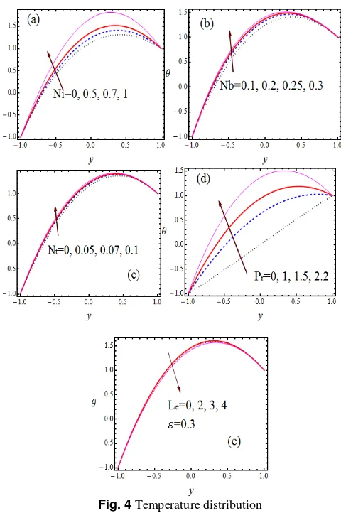
Fig. 4 Temperature distribution

Fig. 3e is displayed to see the effect of the Brownian number N on the _b velocity. The result indicates that velocity of the fluid increases with increasingN . The quite similar effect can be seen in Fig.3f when b

b

N is replaced by Grashof number. Physically, it is true due to the fact that increasing Groshof number means an increase of the buoyancy force, which supports the motion.Fig.3g elucidates the influence of radiation parameter N on ‘u’. It is evident that increasing radiation t

parameter tends to enhance fluid velocity. The effect of the Lewis number L on the dimensionless velocity is displayed in Fig. 3h. It is e

observed that L is lead to increase the fluid velocity in the right of the e

channel. However, this trend is reversed near the walls.

Effects of the parameters N , N , N and P_{1 b t r}on temperature

distribution: Fig.3 illustrates the influences of N , N , N , P and L 1 b t r e

on the dimensionless temperature field. Fig. 4a depicts the effect of radiation parameter on temperature distribution. It is seen that, as expected, temperature field is an increasing function in view of the radiation parameter. Fig. 4b illustrates that temperature profiles shows the same behavior against increasing the value of Brownian number

b

equivalent to increasing momentum diffusivity, which leads to enhance the fluid temperature. Also, Fig. 4e describes that L is not shown much e

influence on temperature distribution. Finally, it is important to note that P shows the significant influence on temperature distribution than _r the other thermal parameters.

Fig. 5 Concentration distribution

Effects of the parameters N , N , N , P and L_{t b 1 r e}on

concentration distribution: Fig. 5 depicts the behavior of the concentration distribution for various values of the parametersN , N , N , P and L . Fig. 5a shows the variation in t b 1 r e

concentration field with different values of thermophoresis parameterN . It depicts that increasing _t N lead to decrease species t

concentration considerably. The quite opposite trend can be seen in concentration profiles if N is replaced by Brownian number t N (See b

Fig.5b). Fig. 5c is graphed to discuss the effect of radiation parameter

1

N on φ. It is observed that increasing N is lead to suppress the ₁ concentration gradually. Fig. 5d shows the effect of P on _r concentration distribution. It reveals that concentration profiles get sharp decrease in centre of the channel with increasingP . Further, it is r

noted that when increasing P from 0 to 1 there is nearly 40% decrease r

in concentration whereas increasing P from 1 to 0.5 there is only 20% _r

(approx) decrease in the same. It means that low values of P gives _r

more influence than higher values of P . Fig. 5e evident that increasing _r Lewis number is tends to enhance fluid concentration gradually.

Effects of the parameters G , I, N , N_{c 1 t} and Pron Volume flow

rate, skin friction, Nusselt number and Sherwood number:

The values of the Volume flow rate (Q), skin friction (τ), wall heat transfer rate (Nu) and wall mass transfer rate (Sh) with various values of local nano-particle Grashof number G , thermophoresis parameter c

(N ), Radiation parameter t N and Prandtl number (1 P ) for fixed r

values of G =3, r G =2, c Re=1, I=1, W =0.01, e N =0.1, t N =0.1, b 1

N =0.5, L =5, , M = 2, e P =2, r Da =2, ω =1, t= π/ 2, ε =0.01 are

listed in Tables 3–10 respectively. Table 3 illustrate the variation in volume flow rate for different values of G and_c N . It depicts that _t

increasing G and _c N is lead to enhance the flow rate gradually. From _t

Table 4 displays the influence of I and N on flow rate distribution, ₁ which indicates that radiation parameter is lead to enhance flow rate whereas the opposite behavior can be noticed with an increase of Inertia coefficient. Table 5 demonstrates the influences of W and e N on skin 1

friction distribution at the wall y=-1. It is observed that an increase of

1

N and W lead to increase the skin friction. Further, from the Table. 6 e

we noticed that an increase of N lead to decrease the skin friction ₁

whereas opposite effect can be seen with increasingW . Influence of _e

r

P and N on Nusselt number distribution at both the walls is displayed ₁

in Tables 7 and 8. It illustrates that increasing N promotes the rate of ₁

heat transfer while the reverse trend can be seen with increasing P at _r

both the walls. Increasing P and r N shows the quite opposite effect on 1

local mass transfer rate distribution, which is displayed in Tables 9 and 10.

Fig. 6 Velocity distribution- Comparsion of HAM solution (G =1, _r R_e =1, W =0.1, M = 2_e )

6. CONCLUSIONS

increasing Grashof number, Brownian motion parameter and radiation parameter. Dimensionless temperature field is an increasing function with increasing thermal parametersN , N , N and P . The increasing _{1 b t r}

values of N , N and P lead to suppress the species concentration _{t 1 r} significantly where as the reverse effect can be noticed by increasing thermophoresis parameterN and L . Radiation parameter lead to _{b e} enhance the skin friction at the wall y=-1 whereas opposite effect noticed at the other wall. Further, W lead to decrease the skin friction e

at both the walls. Radiation parameter lead to enhance rate of heat

transfer at both the walls whereas P tends to suppress the same at both _r the walls. The quite opposite effect can be observed in Sherwood distribution with increasing P and _r N . The results of Siva Shankara 1

Rao and Siva Prasad (2014) can be recovered as a limiting case of our analysis by taking I, N , N , N , L , P ,t b 1 e r ε →0 and Da→ ∞. Further,

proper choice of the parameters and making the boundary conditions similar to present problem for velocity distribution, we note that HAM solutions show very good agreement with the result of Siva Shankara Rao and Siva Prasad (2014) , which is presented in Fig. 6.

Table 3. Effects of Ntand G on Volume flow rate (Q). c

N_t

c

G

0 0.02 0.04 0.06 0.08 0.1

0 0.804336 0.822243 0.840199 0.858200 0.876242 0.894321

2 0.804913 0.784763 0.763116 0.739962 0.715297 0.689111

4 0.824651 0.765926 0.704131 0.639255 0.571284 0.500210

6 0.829880 0.731221 0.627854 0.519764 0.406934 0.289350

Table 4. Effects of N and I on volume flow rate (Q) ₁

N 1

I

0 0.2 0.4 0.6 0.8 1

0 0.458147 0.46474 0.485337 0.522583 0.581578 0.67115

2 0.456262 0.46284 0.483389 0.520549 0.579407 0.668771

3 0.452586 0.459265 0.480152 0.518008 0.578172 0.669944

4 0.450830 0.457528 0.478481 0.516477 0.576913 0.669209

Table 5. Variation on coefficient of Skin friction (C ) for f N and 1 W at the wall y=-1. e

N ₁

e

W

0 0.2 0.4 0.6 0.8 1

0 -0.777670 -0.770202 -0.746781 -0.704114 -0.635834 -0.530861

0.05 -0.75678 -0.74964 -0.727218 -0.686242 -0.620309 -0.518057

0.07 -0.749104 -0.742088 -0.720034 -0.679657 -0.614485 -0.512929

0.1 -0.737907 -0.731077 -0.709572 -0.670065 -0.605938 -0.505149

Table 6. Variation on coefficient of Skin friction (C ) for _f N and 1 W at the wall y=1. e

N 1

e

W

0 0.2 0.4 0.6 0.8 1

0 -1.92938 -1.93824 -1.96584 -2.01552 -2.0937 -2.21149

0.05 -1.81642 -1.82387 -1.847 -1.88838 -1.95287 -2.04861

0.07 -1.76303 -1.76983 -1.79092 -1.82852 -1.88682 -1.97264

0.1 -1.67275 -1.67846 -1.69612 -1.72738 -1.77528 -1.84448

Table 7. Influence of P and _r N on Nusselt number distribution at the wall y=-1 ₁

P r

1

N 0 0.4 0.8 1.2 1.6 2.2

0 -1.000000 -1.46193 -1.95095 -2.47196 -3.32595 -3.95333

0.5 -0.920998 -1.41647 -1.94151 -2.50177 -3.42263 -4.10143

0.7 -0.842922 -1.37542 -1.94020 -2.54380 -3.53858 -4.27433

Table 8. Influence of P and _r N on Nusselt number distribution at the wall y=1 ₁

P r

1

N

0 0.4 0.8 1.2 1.6 2.2

0 -1.000000 -0.5595390 -0.1371920 0.2705980 0.862254 1.24803

0.5 -0.920998 -0.4486880 0.00438378 0.4423450 1.079420 1.49640

1 -0.842922 -0.3354290 0.15165100 0.6230990 1.310820 1.76278

1.5 -0.669275 -0.0683145 0.50940100 1.0704900 1.894760 2.44182

Table 9. Variation on Sherwood number distribution for P and r N at the wall y=-1. 1

P _r

1

N

0 0.4 0.8 1.2 1.6 2.2

0 -0.999612 -0.636981 -0.256859 0.143627 0.789558 1.25558

0.5 -1.061720 -0.677128 -0.273779 0.151552 0.838634 1.33532

0.7 -1.123100 -0.714859 -0.28649 0.165608 0.897065 1.42687

1 -1.259420 -0.791318 -0.299683 0.220101 1.063850 1.67755

Table10. Variation on Sherwood number distribution for P and _r N at the wall y=1. 1

P _r

1

N

0 0.4 0.8 1.2 1.6 2.2

0 -0.985989 -1.33435 -1.67015 -1.99564 -2.46921 -2.77814

0.5 -1.048900 -1.41829 -1.77442 -2.11983 -2.62308 -2.95206

0.7 -1.111180 -1.50323 -1.88131 -2.24824 -2.78365 -3.13441

1 -1.249910 -1.69939 -2.13316 -2.55487 -3.17247 -3.57921

NOMENCLATURE

0

B - transverse magnetic field

1

C ,C - wall concentrations 2

C- the mean value of C and ₁ C ₂

0

C - initial concentration

p

C - specific heat

a 2

k D

L

=

ϕ - permeability parameter B

D - Brownian diffusion coefficient

T

D - thermophoresis diffusion coefficient

2

0 f t 2

0 0

(1 C ) g (T T)L

Gr

=

− ρ β_{µ U} − -local temperature Grashof number

2

p f c 2

c

0 0

( )g (C C)L

G

U

ρ − ρ β −

µ

=

- local nano-particle mass Grashof

number

g - acceleration due to gravity

(

)

2

p _f 0

0

C U L

I= ρ

µ - dimensionless inertia coefficient

k - permeability of the medium K - thermal conductivity of the fluid

T

k is the thermal diffusion ratio

f e

f B

μ L

ρ D

= - Lewis number

2 2 σB L₀

M=

µ - Hartmann number *

B 2 b

D (C C)

N =τ −

ν - Brownian number,

* T 2 t

D (T T)

N

T

τ −

=

ν - thermophoresis parameter 2 2

1

4 L

N K

α

= - radiation parameter

p – pressure

(

μ_Cp

)

f

Pr= _K - Prandtl number

f 0

0

U L Re=ρ

µ -Reynolds number

T – dimensional temperature

1

T , T - wall temperatures ₂

T- mean value of T and ₁ T ₂

0

T - inlet temperature u,v- velocity components

0

U - entrance velocity

0 e

U W

L

Γ

= -Weissenberg number

GREEK SYMBOLS

2

α - mean absorption coefficient

t

β -coefficient of thermal expansion

c

β - coefficient of expansion with concentration

µ - dynamic viscosity

σ- coefficient of electric conductivity 1

ε << - oscillating parameter

θ-dimensionless temperature

φ-dimensionless concentration

f, p

ρ ρ -densities of the base fluid and nanoparticle

p f

( C )ρ - heat capacity of the fluid

p p

( C )ρ - effective heat capacity of the nanoparticle material

ϕ - porosity of the medium

Γ- time constant q

y

∂

∂ - radiative heat flux ω - frequency

APPENDIX

From Section 2, the non-dimensional system of equations is

e r

2

c 1

u u

1 W Hu G

u p 1

y y y

t x Re

G Iu K

∂  ∂ ∂   + − θ     ∂ ∂   − ∂  ∂ ∂   ∂ ∂ _{ } + φ − +  

+

=

+

(9)

p 0

y

∂ = −

∂ (10) 2

2

*

1 b t

2 r

1

Re N N N K

t P y y y y

    ∂θ ∂ θ ∂φ ∂θ ∂θ + θ + + +       ∂

=

∂  ∂ ∂ ∂  (11) 2 2 2 2 t e b N 1 Re

t L

y

N y

 

∂φ ∂ φ ∂ θ

 

∂

=

∂

+

∂  (12)

The corresponding boundary conditions are:

u=0 θ = −1 φ = −1 at y= −1 (13) u=0 θ = + ε1 ei tω φ = + ε1 ei tω at y=1 (14)

The above system of equations (9)-(14) are coupled whose exact solution is not easy to obtain. Therefore, we assume the solution in the form of [See Refs. Cogley et al.(1968) and Muthuraj et al. (2013)]

i t

0 1

u=u (y)+ εeωu (y); θ = θ₀(y)+ εei tωθ₁(y);

i t 0(y) eω 1(y)

φ = φ + ε φ ; p=p (x)₀ + εei tωp (x)₁ (15) Substituting equation (15) in to the equations (9) - (14) we get,

i t 0 1 i t 0 1 e 0 i t 0 1

[u (y) e u (y)]

t

[u (y) e u (y)]

1 W

y

p 1

H[u (y)

x Re y _{[u (y) e u (y)]}

y ω ω ω ∂ + ε ∂  _{∂ + ε}   +   _∂  ∂ ∂ _{ } − _{ }− ∂ ∂ _{∂ + ε }  _∂   

=

+

i t i t

1 r 0 1 c 0

i t i t 2

1 0 1 1

e u (y)] G [ (y) e (y)] G [ (y)

1

Re e (y)] I[u (y) e u (y)] K

ω ω ω ω _{ε θ + ε θ + φ}    +   +ε φ − + ε +    

+

i t i t

1 r 0 1 c 0

i t i t 2

1 0 1 1

e u (y)] G [ (y) e (y)] G [ (y)

1

Re e (y)] I[u (y) e u (y)] K

ω ω ω ω _{ε θ + ε θ + φ}    +   +ε φ − + ε +    

+

2 i t

0 1

i t

0 1 2

r _{i t}

1 0 1

[ (y) e (y)]

[ (y) e (y)] 1

Re y

t P

N [ (y) e (y)]

ω ω ω _{∂ θ + ε θ}    ∂ θ + ε θ ∂   ∂ _{ } + θ + ε θ  

=

i t i t

0 1 0 1

b

[ (y) e (y)] [ (y) e (y)]

N y y ω ω ∂ φ + ε φ ∂ θ + ε θ + ∂ ∂ 2 i t * 0 1 t

[ (y) e (y)]

N K y ω _{∂ θ + ε θ}  +   +  _∂    2 2

i t i t

0 1 0 1

e

[ (y) e (y)] 1 [ (y) e (y)]

Re

t L y

ω ω ∂ φ + ε φ ∂ φ + ε φ ∂

=

∂ 2 2 i t

t 0 1

e b

N [ (y) e (y)]

1

L N y

ω ∂ θ + ε θ ∂

+

i t 0 1

u (y)+ εeωu (y)=0 θ₀(y)+ εei tωθ₁(y)= −1

i t

0(y) eω 1(y) 1

φ + ε φ = − at y= −1

i t

0 1

u (y)+ εeωu (y)=0 θ₀(y)+ εei tωθ₁(y)= + ε1 ei tω

i t i t

0(y) eω 1(y) 1 eω

φ + ε φ = + ε at y=1

The above set of equation gives,

i t

0 1

e i t

1 _{i t}

0 1

i t i t

0 1 r 0 1

i t i t 2

c 0 1 0 1 1

[u (y) e u (y)]

1 W

y

p 1

i e u (y)

x Re y _{[u (y) e u (y)]}

y

H[u (y) e u (y)] G [ (y) e (y)]

1

Re G [ (y) e (y)] I[u (y) e u (y)] K

ω ω ω ω ω ω ω  _{∂ + ε}  _ + _ ∂ ∂ ∂ _{ } ε ω − _{ } ∂ ∂ _{∂ + ε }  _∂    _{− + ε θ + ε θ}    +   + φ + ε φ − + ε +    

=

+

+

2 i t

0 1

i t 2

1

r i t

1 0 1

[ (y) e (y)]

1

i Re e (y) y

P

N [ (y) e (y)]

ω ω ω _{∂ θ + ε θ}    ε ω θ  ∂    + θ + ε θ  

=

i t i t

0 1 0 1

b

[ (y) e (y)] [ (y) e (y)]

N y y ω ω ∂ φ + ε φ ∂ θ + ε θ + ∂ ∂ 2 i t * 0 1 t

[ (y) e (y)]

N K y ω _{∂ θ + ε θ}  +   +  _∂    2 2 2 2 i t 0 1 i t

1 _{i t}

e _{t 0 1}

b

[ (y) e (y)]

1

i Re e (y)

L _{N [ (y) e (y)]}

N y

y

ω ω ω _{∂ φ + ε φ}      ε ω φ _{ } ∂ θ + ε θ    _∂   

∂

=

+

i t 0 1

u (y)+ εeωu (y)=0 θ₀(y)+ εei tωθ₁(y)= −1

i t

0(y) eω 1(y) 1

φ + ε φ = − at y= −1

i t

0 1

u (y)+ εeωu (y)=0 θ₀(y)+ εei tωθ₁(y)= + ε1 ei tω

i t i t

0(y) eω 1(y) 1 eω

φ + ε φ = + ε at y=1

Collection of ε0termsone gets,

2

0 0

e 0 r 0 c 0

2

0 1

du du

d

W Hu G G

dy dy dy

dp0

Iu K Re

2 2

*

0 0 0 0

1 0 b r t r r

2

d d d d

N N P N P K P 0

dy dy dy

dy

 

θ φ θ θ

+ θ + +   + =

 

2 2

t 0

2 2

b

d ₀ N d

0 N

dy dy

φ θ

=

+

The corresponding boundary conditions are:

0

u =0 θ = −₀ 1 φ = −₀ 1 at y= −1

0

u =0 θ =₀ 1 φ =₀ 1 at y=1 Collection of ε1termsone gets,

0

1 1

e 1 1

du

d du du

2W Hu i Re u

dy dy dy dy

 

+ − − ω

 

 

0 1 1 1 dp1

2Iu u G_r G_c Re

dx

−

+

θ + φ

=

2

0 0

1 1 1

1 r 1 b r

2

0 1 t r

d d

d d d

(N i Re P ) N P

dy dy dy dy

dy

d d

2N P 0

dy dy

 θ φ 

θ φ θ

+ − ω θ +  + 

 

θ θ

+ =

e 1

2 2

d _{1 Nt} d ₁

i Re L 0

2 _N 2

dy b dy

φ θ

− ω φ

+

=

with the boundary conditions,

1

u =0 θ =1 0 φ =1 0 at y= −1 1

u =0 θ =₁ 1 φ =₁ 1 at y=1

REFERENCES

Abdul Hakeem A.K., Kalaivanan R., Vishnu Ganesh N., Ganga B., 2014, “Effect of Partial Slip on Hydromagnetic Flow Over a Porous Stretching Sheet With Non-Uniform Heat Source/Sink, Thermal Radiation and Wall Mass Transfer,” Ain Shams Engineering Journal., 5

, pp.913– 922.

http://dx.doi.org/10.1016/j.asej.2014.02.006

Abdollahzadeh Jamalabadi M. Y., 2015, “Entropy Generation In Boundary Layer Flow of Micropolar Fluid Over a Stretching Sheet Embedded in a Highly Absorbing Medium,” Frontiers in Heat and Mass Transfer (FHMT),6, pp. 7 (13 pages)

http://dx.doi.org/10.5098/hmt.6.7

Akbar N.S., Nadeem S., Lee C., Khan Z. H., Ul Haq R., 2013, “Numerical Study Of Williamson Nano-Fluid Flow in an Asymmetric Channel,” Results in Physics,3, pp.161–166.

http://dx.doi.org/10.1016/j.rinp.2013.08.005

Asgari M. A., Mirdamadi H. R., Ghayour M., 2013, “Coupled Effects of Nano Size, Stretching And Slip Boundary Conditions on Nonlinear Vibrations of Nano Tube Coveying Fluid by the Homotopy Analysis Method,” Physica E: Low-dimensional Systems and Nanostructures,

52, pp. 77-85

http://dx.doi.org/10.1016/j.physe.2013.03.031

Buongiorno J., 2006, “Convective Transport In Nanofluids,” Journal of Heat Transfer, 128, pp. 240–50.

http://dx.doi.org/10.1115/1.2150834

Chamkha A.J., Ben-Nakhi A., 2008, “MHD Mixed Convection Radiation Interaction Along a Permeable Surface Immersed in a Porous

Medium in the Presence of Soret and Dufour Effects,” Heat and Mass Transfer, 44, pp. 845–856.

http://dx.doi.org/10.1007/s00231-007-0296-x

Chamkha A.J., Camille I., Khalil K., 2002, “Natural Convection From an Inclined Plate Embedded in a Variable Porosity Medium Due to Solar Radiation,” International Journal of Thermal Sciences, 41, pp.73–81.

http://dx.doi.org/10.1016/S1290-0729(01)01305-9

Cimpean D., Pop I., Ingham D. B., Merkin J. H., 2009, “Fully Developed Mixed Convection Flow Between Inclined Parallel Plates Filled with a Porous Medium,” Transport in Porous Media,77, pp.87– 102.

http://dx.doi.org/10.1007/s11242-008-9264-2

Cogley A. C., Vincenti W. C., Gilles S. E., 1968, “Differential Approximation For Radiative Transfer in a Non-Grey Gas Near Equilibrium,” AIAA J, 16, pp. 551-555.

http://dx.doi.org/10.2514/3.4538

EL-Hakim M.A., Rashad A.M., 2007, “Effect of Radiation on Non-Darcy Free Convection From a Vertical Cylinder Embedded In a Fluid-Saturated Porous Medium With a Temperature-Dependent Viscosity,” Journal of Porous Media, 10, pp. 209–218.

http://dx.doi.org/10.1615/JPorMedia.v10.i2.80

Freidoonimehr N., Rashidi M.M,, Mahmud S., 2015, “Unsteady MHD Free Convective Flow Past a Permeable Stretching Vertical Surface in a Nano-Fluid,” International Journal of Thermal Sciences, 87, pp. 136-145.

http://dx.doi:10.1016/j.ijthermalsci.2014.08.009

Hady F. M., Ibrahim F. S, Abdel-Gaied S. M, Eid M. R, 2012, “Radiation Effect on Viscous Flow of a Nanofluid and Heat Transfer Over a Nonlinearly Stretching Sheet,” Nanoscale Research Letters, 7, pp.229-242.

http://dx.doi.org/10.1186/1556-276X-7-229

Hayat T., Awais M., Asghar S., 2013, “Radiative Effects in a Three-Dimensional Flow of MHD Eyring-Powell Fluid,” Journal of the Egyptian Mathematical Society, 21, pp.379–384.

http://dx.doi.org/10.1016/j.joems.2013.02.009

Hina S., Mustafa M., Abbasbandy S., Hayat T., Alsaedi A.,2014, “Peristaltic Motion of Nanofluid in a Curved Channel,” Journal of Heat Transfer, 136, pp.052001 (7 pp.)

doi: 10.1115/1.4026168

Kakac S., Pramuanjaroenkij A., 2009, “Review of Convective Heat Transfer Enhancement With Nanofluids,” International Journal of Heat and Mass Transfer, 52, pp. 3187–3196.

http://dx.doi.org/10.1016/j.ijheatmasstransfer.2009.02.006

Kothandapani M., Prakash J., 2015, “Effects Of Thermal Radiation Parameter And Magnetic Field on The Peristaltic Motion of Williamson Nanofluids in a Tapered Asymmetric Channel,” International Journal of Heat and Mass Transfer,81, pp. 234–245.

http://dx.doi.org/10.1016/j.ijheatmasstransfer.2014.09.062

Kou H.S., Lu I.T., 1993, “Combined Boundary and Inertia Effects of Fully Developed Mixed Convection in Vertical Channel Embedded in Porous Media,” International Communications in Heat and Mass Transfer, 20,pp. 333-345.