Performance comparison of firefly algorithm i...

Performance comparison of firefly algorithm in

Global Routing Optimization

Abhinandan Khan

, Pallabi Bhattacharya

, Subir Kumar Sarkar

Dept. of Electronics and Telecommunication Engineering, Jadavpur University, Kolkata, India

ABSTRACT

Rapid technological advancements are leading to a continuous reduction in integrated chip sizes. An additional steady increase in the chip density is resulting in device performance improvements as well as severely complicating the fabrication process. The interconnection of all the components on a chip, known as routing, is done in two phases: the global and the local routing phases. This phase affects chip performance significantly and hence researched into extensively. Swarm based algorithms have proven to be quite useful in this domain. It is an emerging area in the field of optimization and this paper presents one such algorithm, the Firefly Algorithm for solving the routing optimization problem. The performance of the algorithm has been compared with other well-known swarm based algorithms. The proposed algorithm shows remarkable improvement in minimizing the interconnect lengths however, computationally, it is much more expensive compared to the other algorithms in question.

Keywords: Swarm Intelligence, Firefly Algorithm, Particle Swarm, Artificial Bee Colony, Global Routing.

I. INTRODUCTION

With the increase in the number of transistors in any electronic circuit, the length of the interconnecting wires also increases. Theseinterconnects have a fixed area thus, making it very difficult to reduce the dependant capacitive and resistive effects. These effects play a significant role in determining the overall chip delay. The only parameter that can be controlled is their length. So for efficient chip fabrication we need an optimum interconnect routing strategy to achieve the minimum possible interconnect length. Thus, arises the essential indigence for efficient routing algorithms in VLSI physical design.The routing problem in VLSI is broadly divided into global and local routing phases. This paper deals with the global routing phase which is essentially a case of finding a Minimal Rectilinear Steiner Tree (MRST) by joining all the terminal nodes, known to be an NP-hard problem [1].

There are several algorithms which return near optimal results [2, 3]. Recently algorithms based on Evolutionary Algorithms (such as Genetic Algorithm [4]) and based on Swarm Intelligence (such as PSO [5], ACO [6], ABC[7], etc.) are being increasingly used in the domain of global routing optimization in VLSI Design.

Swarm Intelligence is a modern optimization techniques that can be used to solve critical real world optimization problems. Swarms use their environment and resources effectively using collective intelligence. Self-organization is the key feature of a swarm. Some of the established and popular optimization techniques based on swarm intelligence are PSO (particle swarm optimization) [5], ACO (ant colony optimization) [6], ABC (artificial bee colony algorithm) [7], FA (firefly algorithm) [8], etc. PSO and ACO have been in existence for more than a decade. On the other hand, ABC and FA are one of the most recently introduced swarm-based algorithms the former being marginally older.

In this work, we propose a global routing algorithm based on the FA and compare the results obtained against those of ABC and PSO. ABC was developed by Karaboga, inspired by the intelligent foraging behaviour of a honey bee hive. PSO was introduced by Kennedy and Eberhart, based on the flocking behaviour of birds. FA, on the other hand was developed by Dr Xin-She Yang at Cambridge University, based on the flashing characteristics and social behaviour of fireflies. Being a decade newer, the FA is much simpler both in concept and implementation compared to PSO. Improvements have been introduced to enhance the optimization capacity of each of the algorithms in our work.

II. PRELIMINARIES

A. Routing in VLSI Systems

Routing in integrated circuits (ICs) is done after the placement phase, which determines the location of each active elementor component of an IC, on a PCB. The task of all routers is the same, working upon some pre-existing polygons consisting cells and their corresponding terminals, known as pins on cells, and optionally upon some pre-existing wiring called pre-routes. Each of these polygons are associated with a net. The primary task of the router is to create geometries such that all terminals assigned to the same net are connected, no terminals assigned to different nets are connected, and all design rules are obeyed. The first step in routing is to determine an approximate course for each net, known as global routing which may optionally include layer assignment. Global routing limits the size and complexity of the following detailed routing steps, which can then be accomplished grid square- by-grid square.

B. Swarm Intelligence

„Swarm‟ as a term is used for an aggregation of animals like fishes, birds and insects like ants, termites and bees performing collective behaviour. The individual agents of such swarms behave without supervision and each of them has a stochastic behaviour due to his/her perception in the neighbourhood. Swarm Intelligence (SI) can be defined as the collective behaviour of swarms which are decentralized and self-organized. Well known examples of SI are bird flocks and colony of social insects like ants and bees. The intelligence of swarm lies in the network of social interactions between the agents themselves and between the agents and their environment. SI is increasingly becoming an area important for research in engineering, science, statistics, bioinformatics, operational research as well as many other disciplines. This is primarily due to the fact that intelligent swarms can solve problems like finding food, dividing labour among nest mates, building nests, etc. which have important counterparts in several real world engineering areas. Two important SI approaches were proposed in the 1990s: one based on colonisation of ants, referred to as ACO by Dorigo et al. [6] and the other based on bird flocking, known as PSO by Kennedy and Eberhart [5]. Both the optimization approaches have been extensively studied over the next two decades and several refined and modified versions have been proposed and successfully applied to find the solution of complex real-world problems across various domains. SI based algorithms proposed in this decade itself include ABC: based on the forging behaviour of honeybees and proposed by Karaboga and FA: based on the path planning of fireflies. Millonas [9] defined some principles in 1999 that need to be satisfied by a swarm to have an intelligent behaviour:

o The proximity principle: a swarm should be able to do simple space and time computations.

o The quality principle: a swarm should be able to respond to quality factors of the environment like the quality of foodstuffs or safety of location.

o The principle of stability: a swarm should not change its mode of behaviour for every fluctuation of the environment. o The principle of adaptability: a swarm must be able to change its behaviour when the investment in energy is worth the

computational price.

C. Artificial Bee Colony Optimization

The ABC algorithm, developed by Karaboga [7], uses the intelligent foraging behaviour of honeybees. In this algorithm, the artificial bees fly around in a search space to find probable food sources (solutions) with high nectar amount (fitness) and finally obtain the food source with the highest nectar (the best solution). The colony of artificial bees consists of three categories of bees: employed, onlooker and scout bees. The number of employed artificial bees is equal to the number of probable food sources as well as the number of artificial onlookers. During each cycle of the search, employed bees search for food sources and return with their nectar amounts (i.e. the fitness of each random solution). They share the nectar and position information of the food sources with the onlookers. The onlooker bees then choose food sources with a probability based on the nectar amounts calculated using equation (3). As and when a food source is exhausted, the visiting employed bee becomes a scout bee. The scout bee searches for a new food source in the search space previously not visited, and when it does find a new food source, the scout becomes employed. These iterative processes are repeated until the termination condition is satisfied. The ABC algorithm has only two input parameters; population of the colony and the counter for a solution that does not change over a predetermined number of cycles. Initially, ABC algorithm generates random solutions using:

xi,j= xj,max − rand 0,1 × xj,max − xj,min … (1)

j. After initialization, each solution of the population is evaluated and the best solution is memorized.Each employed bee produces a new food source in the neighbourhood of its present position by using:

vi,j= xi,j− ∅i,j× xi,j− xk,j … (2)

Here k = {1, 2, 3, …, N} and j = {1, 2, 3, …, N} are randomly chosen indexes; k ≠ i. ∅i,jis a random number in the range

[-1,1]. New solution vi,j is modified with the previous solutionxi,jand a random position in its neighbourhood xi,k.The new

solution vi,j is evaluated and compared to the fitness of xi,j. If the fitness is better than that of xi,j, it is replaced with

xi,jotherwise, vi,j is retained. After the searching process the employed bees share nectar amounts and positions of the food

sources with the onlookers. For each onlooker bee, a food source is chosen by a selection probability. The probability of the food source is calculated:

pi= fitness_i fitness_i … (3)

Herefitnessiis the fitness of the solution or food source, i. Finally, the best solution is memorized and the algorithm repeats

the search processes of the employed bees, onlookers and the scouts until the termination condition is met.

D. Particle Swarm Optimization

Particle swarm optimization is an efficient and well-performing algorithm in the field of optimization, developed by Kennedy and Eberhart in 1995. It is a population based optimization technique. When aschool of birds are searching for food in an unknown space, they share their information within the group, and thus the moving direction of each bird affected by both the global optimist position information and the individual optimist position information. This forms the basis of the algorithm.

In PSO the potential solution to a problem is represented by a particle in the search space, with its position represented by a vector,xid and the rate of change of its position i.e. velocity represented by vidin a D-dimensional search space.The fitness

of each particle is represented by the quality of its position.The particles fly around in the search space with a certain velocity, which (both direction and speed) depends on its own historical best position obtained so far as well as the best position obtained in the swarm. The position as well as the velocity of a particle are modified in an iterative process. The local best position, pid of a particle and the global best position of the swarm, gid is memorized in each iteration. The

velocity and position of a particle are obtained by the following equations:

vi+1= wxi + φ1β1 pi− xi + φ2β2 gi− xi (4)

xi+1= vi+1+ xi (5)

Here the constants, φ1and φ2are responsible for the influence of the individual particle‟s own knowledge (φ1) and that of

the group (φ2), both usually initialised to 2. The variables β1&β2are uniformly distributed random numbers in [0,1] and

piand giare the particle‟s previous best position and the swarm‟s previous best position respectively.The inertia weight w

controls the balance between local and global search performed by the algorithm and is calculated by:

w = 3 − e−200S + R

8× D

2 −1

(6)

Here, S is the size of the swarm, D is the dimension of the optimization problem and R is the relative quality of each solution normalised to [0,1].

E. Firefly Algorithm

The Firefly Algorithm (FA) is a heuristic, stochastic optimization algorithm, based on the social behaviour of fireflies. They communicate with each other using varying flashing patterns that uses bioluminescence. The two fundamental functions of such flashes are to attract mating partners (communication) and to attract potential prey. In addition, flashing may also serve as a protective warning mechanism.

There are certain characteristics in the flashing of real fireflies, such as fireflies are unisex, and thus, every firefly will move towards the more attractive and brighter ones regardless their sex. The relative attractiveness proportional to firefly„s brightness. For a pair of flashing fireflies the one who is less bright will move towards the brighter one. Attractiveness will decrease with increasing space distance between fireflies. If there are no brighter fireflies than a firefly itself, it will move randomly in the search space. And finally the brightness of a firefly is somehow determined by the fitness function value of the objective problem.

In the FA, the process of optimization is simulated with the attraction and the position changing of the individual fireflies. The fitness of the solution is determined by the advantages and disadvantages of the fireflies‟ location, and the process of finding good feasible solutions is presented by the process of the fireflies searching the better locations in the sky in an iterative process. There are two important factors involved: the variation of light intensity and the formulation of the attractiveness. For simplicity, suppose that the attractiveness of a firefly is determined by its brightness and which in turn is associated with the objective function. The higher is the brightness and the better is the location, the more fireflies will be attracted to the direction. If the brightness‟s are equal, the fireflies will move randomly in the search space. The light intensity decreases monotonically as the distance from the source increases and thus attractiveness also decreases monotonically.

In the simplest case for maximum optimization problems, the brightness I of a firefly for a particular location x could be chosen as I x . The attractiveness β is relative, and it should be judged by the other fireflies. Thus, it will differ with the distance ri,jbetween firefly,i and firefly,j. In addition, light intensity decreases with the distance from its source, and light is

also absorbed by the media so light intensity depends on the absorption coefficient of the media. So attractiveness will also vary with the varying degree of absorption.

In the simplest form, the light intensity I(r) will vary according to the inverse square law:

I r = Is

r2 (7)

Here Isrepresents the intensity at the source. For a medium with a fixed light absorption coefficient γ, the light intensity I

will vary with the distance r. That is:

I = Ioe−γr (8)

Here Io is the initial light intensity, In order to avoid the singularity at r = 0 in the expression, the combined effect of both

the inverse square law and absorption can be approximated as the following Gaussian form.

I = Ioe−γr2 (9)

A firefly‟s attractiveness is proportional to the light intensity seen by adjacent fireflies. So we can now obtain the attractiveness β of a firefly as:

β = βoe−γr

2 (10)

In the above equation,βo is the attractiveness at r = 0. It is often faster to calculate1/(1 + r2) than an exponential function. So

the above function, if necessary, can be approximated as:

β = βo

1+γr2 (11)

Characteristic distance is the distance r(=Г=1/γ) over which the attractiveness changes significantly from βo to βoe−1 for

(10) and βo/2 for equation (11).The parameter γ now characterizes the contrast of the attractiveness, and its value is crucial

The distance between any two fireflies, i and j at xiand xj, respectively is the Cartesian distance:

ri,j= xi− xj = dk=1(xik − xjk)2 (12)

Here is xi,kthe kth component of the spatial coordinate,xi of theithfirefly. In 2-D case, we have:

ri,j= (xi− xj )2− (yi− yj)2 (13)

The movement of the firefly i is attracted to another more attractive (brighter) firefly, j is determined by:

xi = xi+ βoe−γri,j

2

(xj− xi) + αεi (14)

Here the second term is due to the attraction and the third term is randomization with α being the randomization parameter, and is a vector of random numbers being drawn from a Gaussian distribution or uniform distribution. For example, the simplest form is εi could be replaced by (rand − ½) where rand is a random number generator uniformly distributed in [0, 1].

For most of our implementation, we can take βo =1 and α [0, 1].

This algorithm has many advantages such asa high convergence rate. Ever agent i.e. firefly works individually and finds a better position for itself in consideration with its current position as well as the position of other fireflies. Thus, it escapes from the local optima and finds a global optimum ina lesser number of iterations. And also it is a robust algorithm. It has two superiorities [11]: automatic subdivision and random reduction. The fireflies in the FA can automatically divide into subgroups so that they swarm around the multimodal optima. This makes it possible for the algorithm to find all thepossible global optima simultaneously. Thus, the algorithm is particularly suitable for nonlinear and multimodal optimization problems. In addition, the randomness is graduallyreduced, using a similar strategy as that used in simulated annealing and this speeds up convergence when the global optimality is approaching.

III. PROBLEM FORMULATION AND APPLICATION OF PROPOSED ALGORITHMS

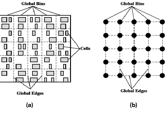
The search space or the grid graph can be represented by a 2D matrix where each element represents a node of the grid graph as shown below. The elements of the matrix corresponding to the nodes that need to be connected, have a value of 1; all the other elements being zero. Thus, it can be seen that all the algorithms require their discrete versions to be implemented as only 0 and 1 are allowed. The problem of global routing optimization can be formulated as the problem of finding an MRST connecting all the terminals or pins, without any severe loss of generality from a grid graph. As illustrated in Fig. 1, the whole routing region is usually partitioned into a number of global bins. Each global bin is represented by a node and each common boundary is represented by an edge in the grid graph. The edges are known as global edges. We have assumed for our work that the capacity of the edges is always greater than the demand or in other words, there is no congestion. The algorithms have been explained below with the help of their pseudocodes. The variables, x and n are used to globally denote the agents and the population of the swarm respectively.

The agents of the swarm in each of the algorithms are initialised based on the matrix used to represent the grid graph.

a1,1 a1,2 a1,3 …… a1,q

a2,1 a2,2 a2,3 …… a2,q

a3,1 a3,2 a3,3 …… a3,q

grid_graph = . . .

. . .

. . .

. . . ap-2,1 ap-2,2 ap-2,3 …… ap-2,q

ap-1,1 ap-1,2 ap-1,3 …… ap-1,q

ap,1 ap,2 ap,3 …… ap,q

A. Pseudocode for ABC

Define objective function f(x), maximum number of iterations, maxit Initialize a population of bees xi(i=1,2,..,n)

Initialize iteration count iter=0 Define a counter, c

While (iter<maxit)

For i = 1:n/2(employed bees) Calculate new solution by eqn. (1) Calculate f(xi) for all i

Calculate pi by eq. (3)

End for

For i = 1:n/2(onlooker bees) Select solution based on pi

Calculate new solution by eq. (2) Calculate f(xi) for all i

Use greedy selection End for

If for a particular xi, f(xi) does not improve until counter

Scout produces new solution using eq. (1) End if

iter = iter +1 End while

B. Pseudocode for PSO

Objective function f(x) = weight of grid_graph Initialise swarm of particles xi(i=1,2,..,n)

Calculate f(xi) for all i and then calculate w

Set pi = f(xi) and gi = minimum of all f(xi)

While (iter<maxgen) For i = 1:n

Calculate vi+1 using eq. (4)

Calculate xi+1 using eq. (5) and modification in [12]

Evaluate f(xi)

If (f(xi)<pi)

Replace pi with f(xi) and update pbest

End If If ((f(xi)<gi)

Replace gi with f(xi) and update gbest

End If End for For i = 1:n

End for iter = iter + 1 End while

C. Pseudocode for FA

Objective function f(x) = weight of grid_graph Initialize a population of fireflies xi(i=1,2,..,n)

Define light absorption coefficient γ While (iter<maxgen)

For i = 1:n For j = 1:i

Light intensity Ii at xi is determined by f(xi)

If (Ii>Ij)

Move firefly i towards j in all d dimensions. (eq. (12)) Else

Move firefly i randomly End if

Attractiveness varies with distance r. (eq. (11)) Evaluate new solutions and update light intensity End for j

End for i

Rank the fireflies and find the current best iter = iter + 1

End while

IV. EXPERIMENTAL SETUP

A total of two different sets of coordinates for terminal nodes are randomly generated for connection. Each algorithm: ABC, PSO and FA, is applied on the two different setups to optimally connect all the terminal nodes mentioned in the sets. Each experiment is run 30 times for each algorithm. The population of swarm is set to 200 and the number of iterations to 100 for each of the SI algorithms. All the terminal node coordinates have been shown in Table I.

TABLE I. EXPERIMENTAL COORDINATES FOR TERMINAL NODES

EXPERIMENT 1: COORDINATES

NO. 1 2 3 4 5 6 7 8 9 10

X 58 32 67 27 99 46 23 16 54 08

Y 80 53 61 66 75 09 92 83 01 45

EXPERIMENT 2: COORDINATES

NO. 1 2 3 4 5 6 7 8 9 10

X 11 31 82 09 26 44 19 41 87 55

Y 97 78 87 40 81 92 27 14 58 15

V. RESULTS AND DISCUSSION

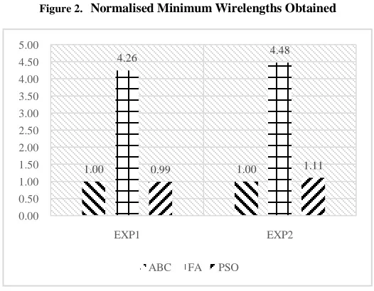
Figure 2. Normalised Minimum Wirelengths Obtained

Figure 3. Normalised Computaional Load

VI. CONCLUSIONS

Routing, both global and local, has a significant impact on the entire chip performance and efficient routing algorithms (with further modifications leading to improved performance) [12] are obviously the key to success in the future in the domain of VLSI physical design. In this work, our main objective has been to obtain the minimumpossible wirelength with the help of a global routing algorithm inspired from fireflies. We have presented an efficient FA based global routing approach and have compared its performance against that of ABC and PSO. Prim‟s Algorithm is used to find the weight of the Steiner trees obtained. It has been suitably modified to work on the incidence matrix and not the weight matrix and also to deal with rectilinear distances instead of only Euclidean distances. The results obtained show that the proposed approach has a potential for further extension. The results of the experiments carried out, demonstrate the feasibility of our algorithm for implementation in VLSI routing optimization and it also has the flexibility to be used in much more complex situations in the future dealing with variable interconnect weights and obstacles in the routing path.Based on simulation results, the solution quality and reliability show the superiority of the FA over the other approaches.

The proposed algorithm however lacks in robustness when compared to the ABC. Also a glaring chink in its armour is its premium computational load requirement. The presented FA has already been modified by the authors of this paper and they have managed to reduce 50% of the time requirement as opposed to their previous work. Further research into this algorithm will hopefully lead to the reduction of runtime for this particular case. Once it becomes comparable to the other evolutionary and swarm based algorithms w.r.t. to the time required to return an optimal result, it will prove to be one of the best solutions to the problem dealt herein.

1.00 1.00

0.75

0.70

0.89 _0.85

0.00 0.20 0.40 0.60 0.80 1.00 1.20

EXP1 EXP2

ABC FA PSO

1.00 1.00

4.26 4.48

0.99 1.11

0.00 0.50 1.00 1.50 2.00 2.50 3.00 3.50 4.00 4.50 5.00

EXP1 EXP2

REFERENCES

[1]. G M Garey and D Johnson, “The rectilinear Steiner tree problem is NP-complete,” SIAM J. Appl. Math, vol. 32, 1977, pp. 826-834,.

[2]. M Pan, and C Chu, “FastRoute 2.0: A High-quality and Efficient Global Routing,” 12th Asia and South Pacific Design Automation Conference, pp. 250–255, 2007.

[3]. Chris Chu and Yiu-Chung Wong, “FLUTE: Fast Lookup Table Based Rectilinear Steiner Minimal Tree Algorithm for VLSI Design,” IEEE Transactions on Computer-Aided Design, vol. 27, no. 1, pages 70-83, January 2008.

[4]. J H Holland, “Adaptation in Natural and Artificial Systems,” University of Michigan Press, Ann Arbor, MI (1975).

[5]. J Kennedy, R Eberhart, “Particle swarm optimization,” IEEE international conference on neural networks, vol. 4, pp. 1942–1948, 1995.

[6]. M Dorigo, A Colorni and V Maniezzo, “Positive feedback as a search strategy,”Technical Report 91-016, Dipartimento di Elettronica, Politecnico di Milano, Milan, Italy, 1991

[7]. D Karaboga,“An idea based on honey bee swarm for numerical optimization,” Technical report. Computer Engineering Department, Engineering Faculty, Erciyes University, 2005.

[8]. X S Yang, “Nature-Inspired Metaheuristic Algorithms,”Luniver Press,(2008).

[9]. M M Millonas, “Swarms, phase transitions, and collective intelligence,” C. G. Langton, Ed., Artificial Life III, Addison Wesley, Reading, MA, 1994.

[10]. Qinghai Bai, “Analysis of particle swarm optimization algorithm,” Computer and Information Science, vol. 3, no. 1, pp. 180-184, 2010.

[11]. XS Yang, Seyyed Soheil Sadat Hosseini, and Amir Hossein Gandomi, “Firefly algorithm for solving non-convex economic dispatch problems with valve loading effect,” Applied Soft Computing,vol. 12, no. 3, pp. 1180-1186, 2012.

[12]. Abhinandan Khan, Sulagna Laha, Subir Kumar Sarkar, “A novel particle swarm optimization approach for VLSI routing,”2013 IEEE 3rd International Advance Computing Conference (IACC), pp. 258-262, 22-23 Feb. 2013.

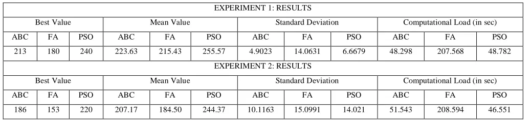
TABLE II. EXPERIMENTAL RESULTS

EXPERIMENT 1: RESULTS

Best Value Mean Value Standard Deviation Computational Load (in sec)

ABC FA PSO ABC FA PSO ABC FA PSO ABC FA PSO

213 180 240 223.63 215.43 255.57 4.9023 14.0631 6.6679 48.298 207.568 48.782

EXPERIMENT 2: RESULTS

Best Value Mean Value Standard Deviation Computational Load (in sec)

ABC FA PSO ABC FA PSO ABC FA PSO ABC FA PSO