Sentiment polarity classification of tweets using a extended dictionary

INTELIGENCIA ARTIFICIAL

http://journal.iberamia.org/

Sentiment polarity classification of tweets using an

extended dictionary

Vladimir Vargas-Calder´

on [email protected]

_{, Nelson A. Vargas S´}

_anchez

[email protected]

, Liliana Calder´

on-Benavides

[email protected]

_{, and Jorge E. Camargo [email protected]}

1

_{Universidad Nacional de Colombia}

_{Universidad Aut´}

_{onoma de Bucaramanga}

_Fundaci´

_{on Universitaria Konrad Lorenz}

Abstract With the purpose of classifying text based on its sentiment polarity (positive or negative), we pro-posed an extension of a 68,000 tweets corpus through the inclusion of word definitions from a dictionary of the Real Academia Espa˜nola de la Lengua (RAE). A set of 28,000 combinations of 6 Word2Vec and support vector machine parameters were considered in order to evaluate how positively would affect the inclusion of a RAE’s dictionary definitions classification performance. We found that such a corpus extension significantly improve the classification accuracy. Therefore, we conclude that the inclusion of a RAE’s dictionary increases the semantic relations learned by Word2Vec allowing a better classification accuracy.

ResumenCon el prop´osito de clasificar texto basado en su polaridad de sentimiento (positivo o negativo), en este art´ıculo se propone una extensi´on de un corpus de 68.000 tweets mediante la inclusi´on de palabras pertenecientes a definiciones de un diccionario de la Real Academia Espa˜nola de la Lengua (RAE). Un cojunto de 28.000 combinaciones de 6 par´ametros de Word2vec y M´aquinas de Soporte Vectorial fueron considerados para evaluar qu´e tan positivamente se afecta el desempe˜no de la clasificaci´on. Se encontr´o que al hacer la expansi´on propuesta se incrementan las relaciones aprendidas en Word2vec, permitiendo obtener una mayor precisi´on en la clasificaci´on.

Keywords: Corpus extension, Word2Vec, Support vector machine, Sentiment analysis, Polarity, Semantics.

Palabras Clave: Extensi´on de corpus, Word2Vec, M´aquinas de soporte vectorial, An´alisis de sentimientos, Polaridad, Sem´antica.

1

Introduction

Sentiment analysis is one of the most challenging tasks in machine learning applied to text. One of its most active branches is text classification by sentiment polarity, which refers to the positivity or negativity of the sentiment represented by the text. There are prominent difficulties in classifying text by polarity when text is too short, as it is the case in Twitter in which text does not exceed 140 characters. To overcome these difficulties, this paper presents an extension to the TASS (sentiment analysis workshop of the Spanish society for natural language processing) General corpus [1] (hereafter just corpus). The TASS corpus consists of a set of tagged tweets by polarity, and the extension consists in including definitions from the Spanish Real Academy’s dictionary (RAE) to the set of texts from which sentiment analysis algorithms learn. In this work, we compared a sentiment analysis algorithm trained with tweets with another trained with both tweets and RAE’s dictionary definitions. The reason for extending the corpus with RAE’s dictionary definitions is that they provide semantic relations between

ISSN: 1137-3601 (print), 1988-3064 (on-line) c

words. The technique of extending a corpus composed of short texts is used to expand the context. Applying this technique allows to improve text classification by polarity, as shown by the studies in [2, 3]. Additionally, some text domains grow at such fast rates that it is practically impossible to maintain the training data updated. Therefore, using related domains with tagged text is a solution that has been lately used to overcome scarce tagged data. This is called cross-domain text classification, and has shown preliminary results. Nevertheless, some procedures have been developed and tested, and the results have improved, such as the work of Wang et al. [4], where Wikipedia is used to propagate labels between two different text domains which captures common words and semantic concepts contained in the documents; as well as the work of Mouri˜no et al. [5], where the concept of cross-language concept matching is proposed to perform cross-language text classification, which is based on the representation of concepts using Wikipedia correspondence of concepts in different languages.

The vast majority of research has been done using text in English. In spite of scarce research using text in Spanish, there has been recent and steady progress. However, it is evident that sentiment analysis research needs more attention on Spanish corpora since Spanish is a more inflected language than English [6]. Few studies, such as the one by Ortega et al. have deepen in Spanish text domain extension [7].

Some other relevant works using Spanish corpora for sentiment analysis have been based on the polarity analysis of lexicons. This is the case of the research by Pablos et al., in which Word2Vec is used to automatically create a lexicon dictionary with associated polarities [8]. Also, Cruz et al. rank lexicons by their impact on the task of text classification by polarity [9].

Other works have tackled some specific problems in the industry, e.g. [10, 11], while some research, such as [12], have enhanced results of binary classification in sentiment analysis, as well as in topic classification using the concept of maximum entropy. Concerning informal text, including the one found on the Internet, Mosquera et al. proposed preprocessing methods to regularize and normalize such texts for a better performance in sentiment analysis tasks.

In this paper, we propose a model based on Word2Vec that allows to represent words as vectors from an extended Twitter corpus with RAE’s dictionary definitions. The model detects word’s polarities given their occurrences in tweets tagged with positive or negative polarities. The main goal of this study was not to obtain high accuracy in text classification by polarity, but to measure the profit of classification accuracy when RAE’s dictionary definitions are included in the training process of Word2Vec.

In section 2 we present the Word2Vec method, as well as review support vector machines. Section 3 shows the details of TASS corpus, the tool built to obtain RAE’s dictionary definitions, and also shows a flow diagram of the proposed model for sentiment analysis. In section 4 we give and analyze the main results of our research. Finally, in section 5 we discuss the results and give some perspectives for future research, and we present the conclusions of this paper.

2

Theoretical Framework

In this section we present the tools used in our method of corpus extension. In order to do that we define some key concepts. A corpus is a collection or set of texts (also called documents) that share a topic or common origin. The vocabulary of this corpus is the set of all words contained in the corpus. In general, when texts are informal, there are sequences of characters that are not official words, but have a concrete meaning in a given cultural context. Thus, the concept of word is generalized by the concept of token, which is defined as any sequence of characters with a meaning. We also define the context of a word, referred as target word, as the set of words that are near to the target word. Specifically, the context has a size 2c, which means that all the words that are at a maximum distance ofcof the target word are context words.

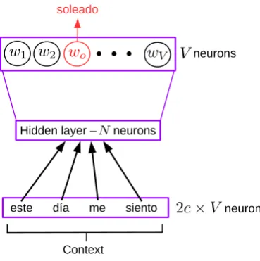
Example 1 Consider the sentence “en este d´ıa soleado me siento genial” (I feel great on this sunny day). Let “soleado” (sunny) be the target word. Ifc= 2, then the context of “soleado” is the set of words at a maximum distance of 2 from the target word. Thus the context is{“este”, “d´ıa”, “me”, “siento”}.

2.1

Word2Vec

One of the essential problems in automatic text analysis is to represent it numerically to establish quantitative relationships between words, phrases or longer texts. Mikolov et al. proposed the Word2Vec method, which sup-ports the construction of embedded vector spaces whose dimensions harbor the semantic and syntactic meanings of words [13].

V, then its hot-vector is

w2= (0,1,0, . . . ,0), (1)

and has V components. Hence, Word2Vec maps words from the vocabularyV to hot-vectors ofV components, and later on, builds an embedded vector space of N dimensions in which each word wi is paired with a vector ωi∈RN. In generalN V, meaning that the embedded vector space has a much lower dimensionality than the number of words in the vocabulary (usuallyN/V <10−2).

The way in which the embedded vector space is built is via a neural network (NN). This NN learns the co-occurrences of words that share similar contexts. There exist two different possible configurations of the NN used by Word2Vec: CBOW and Skip-gram. CBOW means continuous bag of words, and predicts a target word given context words. This is, suppose that there are sentences in which a target wordwo is present. Beforehand, a context size cis set (to exemplify, supposec= 1). This means that the target wordwo has contexts composed of two context words wbefore and wafter, that are situated before and afterwo, respectively. Thus, the CBOW configuration is a NN whose input are the hot-vectors ofwbefore andwafter, and tries to predict the hot-vector of the target wordwo. On the other hand, the Skip-gram configuration takes as the input the hot-vector of the target wordwo and tries to predict its context wordswbefore andwafter.

For this work we selected the CBOW configuration that consisted of three neuron layers shown from bottom to top in Figure 1: the input, hidden and output layers. Again, if we suppose that the context has a size of 2c, then the input layer contains 2crows of V neurons in order to take the hot-vectors of the 2ccontext words. Each row of V neurons is fully connected to a hidden layer of N neurons. These connections are represented by 2c N×V matrices that relate each context word’s hot-vector with theN-neurons hidden layer. Finally, the hidden layer is fully connected to the output layer, that containsV neurons. These connections are represented by aV ×N matrix. Ideally, given a context, the NN should predict the target word’s hot-vector. In the case of Figure 1, there are 4 context words and the correct target word is “soleado”.

este día me siento

Context

Hidden layer – neurons soleado

neurons neurons

Figure 1: CBOW configuration of Word2Vec’s NN using example 1.

The way in which the NN represents a wordwias a vector in anN-dimensional vector space is by associating thei-th row of the connection matrix between the hidden and output layers with thei-th word. The reason why this works is that words that appear in similar contexts must have similar vector representations. This is achieved by defining the NN’s error function as

2.2

Non linear support vector machine

A support vector machine (SVM) is a supervised learning method used for classification. This method consists in learning particular features of numerical objects that belong to different classes. The learning process starts with a training dataset

S:={(x1, y1),(x2, y2), . . . ,(xm, ym)}, (3) where xi ∈X⊂Rp and yi ∈Y= {−1,1} for alli= 1, . . . , m. Note that there are only two tags because we performed binary classification (positive or negative polarity). Moreover, the observationsxihavepfeatures.

A SVM looks for a pair of parametersw∈Rp, b∈Rsuch that the hyperplane

{x∈Rp:f(x) :=hw,xi+b= 0} (4)

given by a discriminant functionf, divides the spaceRpin two semi-spaces: one that contains all the observations with tag -1, and the other one that contains the ones with tag 1. This means that the SVM builds two connected regions inRp, one for each class. Also, the distance from the hyperplane to the nearest observation’s vector from each class must be maximized. These nearest vectors are called support vectors. The method so far presented is called linear SVM, and rarely is useful to classify real data.

To treat real data, Vapnik et al. proposed to map the set of observationsXto a higher-dimensionality space, called the feature space F ⊂ Rp˜, where ˜p > p, so that the observations are linearly separable in F [15]. This means that inRp˜there exists a hyperplane that divides the space as desired. This map is built with a function Φ :Rp→Rp˜that allows a re-definition of the discriminant function as

f(x) =hw,Φ(x)i+b, (5)

wherew∈Rp˜. To make this learning process computationally efficient, a kernelk(x,x0) is defined as

k(x,x0) :=hΦ(x),Φ(x0)i. (6)

If we writew= m

X

i=1

αixi, whereαi∈R, i= 1,2, . . . , m, then

f(x) = m

X

i=1

αik(x,xi) +b. (7)

The reason why this is computationally efficient is that it is not necessary to explicitly compute Φ in order to computek(x,x0). This is the case of the Gaussian kernel, or radial basis functions kernel (RBF), defined by

kRBF(x,x0) = exp(−γ||x−x0||), (8) whereγ ∈R+ is a free parameter that represents the influence that a vector x has over a vector x0. In other words, sincekRBF is a similarity measure between two vectors, then γ is the inverse radius of influence of the support vectors. If this radius is small, then the SVM-RBF allows non-connected regions inRpfor each class.

It can be shown that the function ΦRBFcorresponding to the kernelkRBF(x,x0) maps the observations to a vector space of infinite dimension [16], i.e.:

ΦRBF:_Rp→R∞, (9)

which eases, in theory, the task of finding the hyperplane (in R∞) that divides the observations from different classes.

In our work, we selected the RBF kernel because it is able to separate non-linear data in high-dimensional spaces, which is not necessarily the case of linear kernels. However, in the SVM it is possible to change the kernel by other non-linear kernels.

3

Method and Materials

Vocabulary

TASS corpus Crawler RAE

Mongo DB

Preprocessing

Word2Vec

With RAE Without RAE

SVM-RBF

Figure 2: Flow diagram of the proposed model.

3.1

TASS corpus

TASS is a yearly-released workshop organized by the Spanish society for the natural language processing (SEPLN). TASS consists of activities related to sentiment analysis. Participants have access to tagged corpus that contains over 68,000 tweets in Spanish written by around 150 influent people (famous people or celebrities) from the world of politics, economy, media and culture, collected from November, 2011 to March, 2012 [1]. Figure 3 shows the tweet length in characters distribution. The figure exhibits the fact that this group of people tend to use the maximum number of characters to express their opinions.

Figure 3: Histogram with tweets length distribution measured in characters.

together in two main classes: the positive class (P+ y P), and the negative one (N+ y N). This means that the set of tagged tweets has around 5100 tweets, corresponding to 70% of the initial tagged tweets.

The corpus is originally written in XML format. To read it and manage its information efficiently, the Python’s Beautiful Soup library was used [17]. Additionally, the corpus was stored in a Mongo database using Python’s Pymongo library with the objective of reading and writing information rapidly [18].

3.2

Crawler

With the purpose of extending the TASS corpus with RAE’s dictionary definitions, a crawler was built in order to obtain such definitions. The process consisted in searching each token from the TASS corpus’ vocabulary and to obtain the first definition, which is commonly the most used one. These definitions were stored in a collection of the Mongo database.

In pursuance of building the crawler, Selenium was used [19]. This tool allows to automatize multiple processes in web browsers. In our case, we automatized the process of typing each token in the search bar of RAE’s dictionary, and to obtain the definitions of those tokens found in the dictionary.

It is important to point out that most of the tokens are not words present in the RAE’s dictionary, as shown in Figure 4. This figure is a heat map, or a 2D histogram, in which dark (light) zones correspond to many (few) tweets, and whose the distribution of number of tokens per tweet, as well as the portion of those tokens found in RAE’s dictionary. If a tweet is on the black, green or cyan line means that every, half or a quarter of its tokens are found in RAE’s dictionary, respectively. Therefore, Figure 4 shows that most tweets have from a quarter to half of their tokens present in RAE’s dictionary.

Figure 4: 2D histogram of number of tokens per tweet and the percentage of them that are found in RAE’s dictionary (DRAE). Black, green and cyan lines correspond to 100%, 50% and 25%, respectively.

3.3

Preprocessing

The content of each tweet was modified following 5 preprocessing steps: cleaning, automatic correction, regular-ization, tokenization and lemmatization.

Cleaning

computing time for their processing. Normally, these words are articles, pronouns, prepositions, among others. To remove them from the tweets, the NLTK library was used [20].

Automatic correction

In order to avoid words written with mistakes, Language Tool’s API for Python was used [21]. Language Tool verifies grammar, orthography and style in a text. This tool allowed us to automatically correct words and structures found in tweets that were badly written.

Regularization

Although uppercase might be useful for some natural language processing applications [22], a good practice to analyze text using Word2Vec is to lowercase all characters. Also, the tokenizer that was used (see section 3.3) in this work required to remove accents from characters because it interprets them as token separators, i.e., words like “canci´on” (song) were tokenized as [“canci”, “on”].

Tokenization

Tokenization is the process of converting a string of characters to a list of tokens. The automation of this procedure is implemented by NLTK’s tokenizer TweetTokenizer [20].

Lemmatization

The last step of preprocessing is lemmatization. Here, tokens that are actual words are replaced by their lemma. For example, the token “canciones” was replaced by “canci´on”. This task was performed using the pattern library from the computational linguistics group CLiPS [23]. The objective of this step was to reduce the vocabulary so that sentences containing words with the same lemma would be related by their respective embedded vector.

3.4

Experiments

We designed a model for training Word2Vec and training the SVM-RBF classifier, and measured its performance with the classification accuracy metric. The model depends on some training parameters, denoted by a tuple θ. Therefore, the model is a functionM : Θ→[0,1], where Θ is the set of all possible parameters of Word2Vec and SVM-RBF. Moreover,M takes on values from 0 to 1, where 0 corresponds to 0% of classification accuracy, and 1 to 100%.

The process of training the model with a tuple of parameters and obtaining its corresponding classification accuracy is called the execution of an experiment. Each experiment was carried out in two stages. The first one consists in training Word2Vec’s NN, and the second one consists in training and testing the SVM-RBF classifier. Furthermore, Word2Vec’s NN training was performed in two different ways: the first one used both tweets and RAE’s dictionary definitions as training sentences, and the second one used only tweets (see dashed line zone in Figure 2). This allows to define a first parameter θ1 = 0,1, where 0 represents the first way and 1 the second one. A second parameterθ2= 20,40,60,80,100 was called the minimum number of occurrences, and implies that vector representations of tokens that appear less thanθ2 times in all the corpus were not built. θ3 = 3,5,7,10 was the third parameter, and corresponds to the maximum distance from the target word that a token has to have in order to be in its context (i.e. θ3 =c). The fourth parameter,θ4= 30,60,90,120,150,190,220,250, was the embedded vector space dimension, this is, the number of neurons in the hidden layer of Word2Vec’s NN.

Once we obtained the tokens’ vector representations, we built the tweets’ vector representations for those tweets that were tagged with polarity in the corpus. This was done by taking the average of the vector representation of the tokens that composed each tweet. However, these construction of tweets’ vector representation was not done for every tagged tweet. We introduced a fifth parameter θ5= 4,5,6,7,8,9,10 called the minimum number of tokens per tweet, and the vector representations were not built for tweets with less thanθ5tokens. This means that θ5 limited the number of tweets that served as observations for the training and testing of the SVM-RBF classifier. In particular, the number of tweets varied from 1,112 to 4,074 (because bothθ5andθ2affect the number of tweets), and these were split in 80% for training and 20% for testing. In order to keep the classes with the same amount of tweets, tweets were randomly eliminated from the class containing the most tweets until both classes had the same number of tweets. It should be noted that from the first stage the tweets were split into these two sets.

takes the valuesθ7= 10−2,10−1,100,101,102. The latter, trades off misclassification of training examples against simplicity of the discriminant surface. Low values ofθ7 generate smooth surfaces, while large values grants the algorithm the power to select more training vectors as support vectors, and build more complex discriminant surfaces.

In conclusion, the space of parameters Θ is the set of all possible tuples θ = (θ1, θ2, . . . , θ7) made with the mention values for each parameter. Therefore 56,000 experiments were executed in total. Thus, 28,000 experiments were executed without using RAE’s dictionary definitions and 28,000 using it.

We define ˜Θ as the set of all possible tuples ˜θ= (θ2, θ3, . . . , θ7). The reason why we carried out this brute force work of many experiments was the construction and comparison of two classification accuracy distributions defined over ˜Θ: one corresponding toθ1 = 0 (without RAE) and the other one corresponding to θ1 = 1 (with RAE). These distributions helped us answer the question of how probable is thatM(θ|θ1=1)> M(θ|θ1=0) when we choose ˜θrandomly, whereθ=θ1⊕˜θ(⊕is used as concatenation symbol). In other words, the distributions determined if it is the case that extending the corpus with RAE’s dictionary definitions to the set of training sentences of Word2Vec’s NN improve the classification accuracy of polarities.

4

Results and Analysis

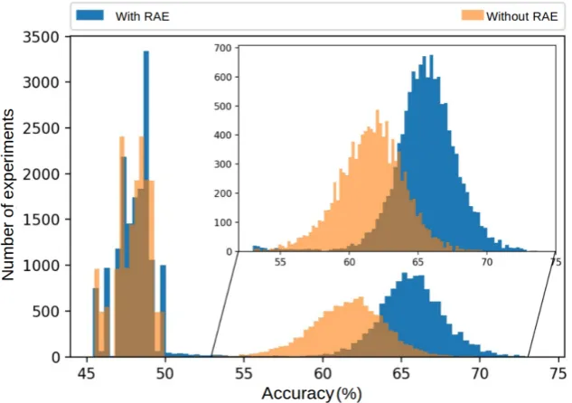
The classification accuracy distributions corresponding to experiments that only used tweets, and experiments that used both tweets and RAE’s dictionary definitions as training sentences for Word2Vec’s NN are shown in Figure 5.

Figure 5: Classification accuracy distributions for experiments with and without RAE’s dictionary defi-nitions incorporated to the training sentences of Word2Vec’s NN.

Figure 5 has two outstanding regions: the one corresponding to accuracy values greater or equal than 50% and the one with accuracy values lower than 50%. Both regions are interesting, but the first one offers over-whelming hints that using RAE’s dictionary definitions within the set of training sentences of Word2Vec’s NN improves classification accuracy significantly. In this region, both distributions are gaussian and contain 12,120 and 10,989 experiments that use and do not use RAE’s dictionary definitions, respectively. Additionally, the gaussian distributions point out that, in average, using RAE’s dictionary definitions as part of the training sen-tences of Word2Vec’s NN improves the accuracy between 4%-5% with respect to the accuracy obtained when one does not use these definitions. Also, it is notable that the width of the distribution corresponding to experiments that incorporate RAE’s dictionary definitions is lower than the width of the distribution of experiments that do not include them, which shows less dispersion and greater stability in the results.

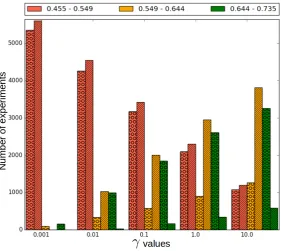
is significantly worse than a random classifier. A possible explanation of this phenomenon is that for some values ofγandθ7, the SVM-RBF classifier generates very simple hypersurfaces that prevent a correct discrimination of non connected regions corresponding to a single polarity. This is evident from Figure 6, which shows a histogram of experiments grouped by the value ofγ for three intervals of accuracy. The larger γ, the more complex and versatile the hypersurfaces are, and the higher the classification accuracy is (green bars). Conversely, the lower

γ, the lower the classification accuracy is (pink bars).

Figure 6: Histogram of number of experiments with different values ofγfor three intervals of low (0.455-0.549), medium (0.549-0.644) y high (0.644-0.735) accuracies, shown with pink, yellow and green colors, respectively. Dotted (lined) bars correspond to experiments that use (do not use) RAE’s dictionary definitions as part of Word2Vec’s NN training sentences.

A similar behaviour was found with the parameterθ7. Therefore, it is clear that the classifier is very sensible to the parameters γ =θ6 andθ7. Since the best classification results were obtained with the highest values of

θ6andθ7, we built a comparison between experiments that used and did not use RAE’s dictionary definitions as part of Word2Vec’s NN training sentences, taking into account all the experiments with parameters θ6 = 1,10 andθ7= 10,100. The comparison was made in the following way: A histogram of the following set was made:

{M(θ|θ1=1)−M(θ|θ1=0) :θ∈Θ∧θ6= 1,10∧θ7= 10,100}.

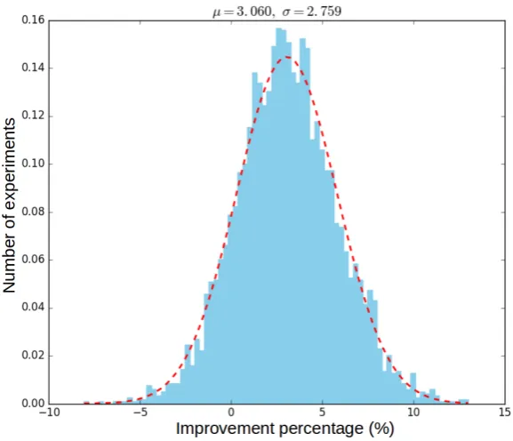
In other words, the comparison was made by producing a histogram of the improvement percentage in the clas-sification accuracy when RAE’s dictionary definitions were included as part of Word2Vec’s NN training sentences. This is, given a tuple of parameters, the histogram shown in Figure 7 tells the probability that the accuracy obtained when using RAE’s dictionary definitions is higher than when they are not used.

Figure 7 shows that the improvement percentage in classification accuracy is statistically significant (to 1σ). For the selected subset of experiments, this improvement is, in average, of 3%.

5

Conclusions

Figure 7: Normalized histogram of the number of experiments by the improvement percentage obtained when RAE’s dictionary definitions were included as part of Word2Vec’s NN training sentences. The red line shows a gaussian curve with mean 3.060% and standard deviation 2.759%.

selected. Furthermore, it is clear that the accuracy percentages of the binary polarity classification are low and can be improved including a lexicon polarity dictionary in order to build the vector representations of tweets more adequately. Finally, it is important to verify that this improvement does not only occur with the Word2Vec method, but also with other representation models (e.g. GloVe) of words as embedded vectors. Also relevant is to measure the impact of including RAE’s dictionary definitions as part of Word2Vec’s NN training sentences in different corpora; for instance corpora with longer and better written texts in order to ensure that a larger percentage of these texts’ tokens are found in RAE’s dictionary, which could be helpful for automatic news analysis like predicting stock prices with financial news articles [26].

References

[1] Eugenio Mart´ınez C´amara, Miguel ´A. Garc´ıa Cumbreras, Julio Villena Rom´an, and Janine Garc´ıa Morera. Tass 2015 – the evolution of the spanish opinion mining systems. Procesamiento del Lenguaje Natural, 56:33–40, 2016.

[2] Yuan Man. Feature extension for short text categorization using frequent term sets. Procedia Computer Science, 31:663 – 670, 2014. 2nd International Conference on Information Technology and Quantitative Man-agement, ITQM 2014. URL:http://www.sciencedirect.com/science/article/pii/S1877050914004918, doi:http://dx.doi.org/10.1016/j.procs.2014.05.314.

[3] S. Lee, J. Kim, and S. H. Myaeng. An extension of topic models for text classification: A term weighting approach. In2015 International Conference on Big Data and Smart Computing (BIGCOMP), pages 217–224, 2015. doi:10.1109/35021BIGCOMP.2015.7072834.

[4] Pu Wang, Carlotta Domeniconi, and Jian Hu. Cross-domain text classification using wikipedia. IEEE Intelligent Informatics Bulletin, 9(1):5–17, 2008.

[5] Marcos Antonio Mouri˜no Garc´ıa, Roberto P´erez Rodr´ıguez, and Luis Anido Rif´on. Wikipedia-based cross-language text classification.Information Sciences, 406–407:12 – 28, 2017. URL:http://www.sciencedirect. com/science/article/pii/S0020025517306680,doi:https://doi.org/10.1016/j.ins.2017.04.024.

[7] F. Javier Ortega, Jos´e A. Troyano, Ferm´ın L. Cruz, and Fernando Enr´ıquez. Enriching user reviews through an opinion extraction system. Procesamiento del Lenguaje Natural, 55:119–126, 2015.

[8] Aitor Garc´ıa-Pablos and Germ´an Rigau. Unsupervised word polarity tagging by exploiting continuous word representations. Procesamiento del Lenguaje Natural, 55:127–134, 2015.

[9] Ferm´ın L. Cruz, Jos´e A. Troyano, Beatriz Pontes, and F. Javier Ortega. Ml-senticon: Un lexic´on multiling¨ue de polaridades sem´anticas a nivel de lemas. Procesamiento del Lenguaje Natural, 53:113–120, 2014.

[10] Flor Miriam Plaza-del Arco, M. Teresa Mart´ın-Valdivia, Salud Mar´ıa Jim´enez-Zafra, M. Dolores Molina-Gonz´alez, and Eugenio Mart´ınez-C´amara. Copos: Corpus of patient opinions in spanish. application of sentiment analysis techniques. Procesamiento del Lenguaje Natural, 57:83–90, 2016.

[11] L. Alfonso Ure˜na L´opez, Rafael Mu˜noz Guillena, Jos´e A. Troyano Jim´enez, and Mar´ıa-Teresa Mart´ın Valdivia. Attos: An´alisis de tendencias y tem´aticas a trav´es de opiniones y sentimientos. Procesamiento del Lenguaje Natural, 53:151–154, 2014.

[12] Fernando Batista and Ricardo Ribeiro. Sentiment analysis and topic classification based on binary maximum entropy classifiers. Procesamiento del Lenguaje Natural, 50:77–84, 2013.

[13] Tomas Mikolov, Ilya Sutskever, Kai Chen, Greg S Corrado, and Jeff Dean. Distributed representations of words and phrases and their compositionality. Advances in neural information processing systems, pages 3111–3119, 2013.

[14] Yoav Goldberg and Omer Levy. word2vec explained: Deriving mikolov et al.’s negative-sampling word-embedding method, 2014.

[15] Bernhard E. Boser, Isabelle M. Guyon, and Vladimir N. Vapnik. A training algorithm for optimal margin classifiers. In Proceedings of the Fifth Annual Workshop on Computational Learning Theory, COLT ’92, pages 144–152, New York, NY, USA, 1992. ACM. URL: http://doi.acm.org/10.1145/130385.130401, doi:10.1145/130385.130401.

[16] Nello Cristianini and John Shawe-Taylor. An Introduction to Support Vector Machines and Other Kernel-based Learning Methods. Cambridge University Press, 1st edition, 2000.

[17] Leonard Richardson. Beautiful soup documentation, 2015. URL: https://www.crummy.com/software/ BeautifulSoup/bs4/doc/[cited February 27, 2017].

[18] MongoDB Inc. Pymongo 3.4.0 documentation. URL: https://api.mongodb.com/python/current/ #about-this-documentation[cited March 5, 2017].

[19] Sagar Shivaji Salunke. Selenium Webdriver in Python: Learn with Examples. CreateSpace Independent Publishing Platform, 1st edition, 2014.

[20] Steven Bird, Ewan Klein, and Edward Loper. Natural language processing with Python: analyzing text with the natural language toolkit. O’Reilly Media, Inc., 2009.

[21] Steven Myint. Language check. URL: https://pypi.python.org/pypi/language-check [cited March 10, 2017].

[22] Konstantin Buschmeier, Philipp Cimiano, and Roman Klinger. An impact analysis of features in a classifi-cation approach to irony detection in product reviews. Proceedings of the 5th Workshop on Computational Approaches to Subjectivity, Sentiment and Social Media Analysis, pages 42–49, 2014.

[23] Tom De Smedt and Walter Daelemans. Pattern for python. Journal of Machine Learning Research, 13:2063– 2067, 2012.

[24] Radim ˇReh˚uˇrek and Petr Sojka. Software framework for topic modelling with large corpora. InProceedings of the LREC 2010 Workshop on NewChallenges for NLP Frameworks, pages 45–50, Valletta, Malta, 2010. ELRA.

[25] F. Pedregosa, G. Varoquaux, A. Gramfort, V. Michel, B. Thirion, O. Grisel, M. Blondel, P. Prettenhofer, R. Weiss, V. Dubourg, J. Vanderplas, A. Passos, D. Cournapeau, M. Brucher, M. Perrot, and E. Duchesnay. Scikit-learn: Machine learning in Python. Journal of Machine Learning Research, 12:2825–2830, 2011.