Learning Hidden Variable Networks: The Information Bottleneck Approach

Learning Hidden Variable Networks:

The Information Bottleneck Approach

Gal Elidan [email protected]

Department of Engineering and Computer Science The Hebrew University

Jerusalem, 91904, Israel

Nir Friedman [email protected]

Department of Engineering and Computer Science The Hebrew University

Jerusalem, 91904, Israel

Editor: David Maxwell Chickering

Abstract

A central challenge in learning probabilistic graphical models is dealing with domains that involve hidden variables. The common approach for learning model parameters in such domains is the expectation maximization (EM) algorithm. This algorithm, however, can easily get trapped in sub-optimal local maxima. Learning the model structure is even more challenging. The structural EM algorithm can adapt the structure in the presence of hidden variables, but usually performs poorly without prior knowledge about the cardinality and location of the hidden variables. In this work, we present a general approach for learning Bayesian networks with hidden variables that overcomes these problems. The approach builds on the information bottleneck framework of Tishby et al. (1999). We start by proving formal correspondence between the information bottleneck objective and the standard parametric EM functional. We then use this correspondence to construct a learning algorithm that combines an information-theoretic smoothing term with a continuation procedure. Intuitively, the algorithm bypasses local maxima and achieves superior solutions by following a continuous path from a solution of, an easy and smooth, target function, to a solution of the desired likelihood function. As we show, our algorithmic framework allows learning of the parameters as well as the structure of a network. In addition, it also allows us to introduce new hidden vari-ables during model selection and learn their cardinality. We demonstrate the performance of our procedure on several challenging real-life data sets.

Keywords: Bayesian networks, hidden variables, information bottleneck, continuation, variational

methods

1. Introduction

Probabilistic graphical models have been widely used to model real world domains and are par-ticularly appealing due to their natural interpretation. Despite extensive research in learning these models from data (Pearl, 1988; Heckerman, 1998), learning with hidden (or latent) variables has

remained a central challenge in learning graphical models in general, and Bayesian networks in particular. Hidden entities play a central role in many real-life problems: an unknown regulating mechanism can be the key to complex biological systems; correlating symptoms might hint at a hid-den fundamental problem in a diagnostic system; an intentionally masked economic power might be the cause of related financial phenomena. Indeed, hidden variables typically serve as a summa-rizing mechanism that “captures” information from some of the observed variables and “passes” this information to some other part the network. As such, hidden variables can simplify the network structure and consequently lead to better generalization.

When learning the parameters of a Bayesian network with missing values or hidden variables, the most common approach is to use some variant of the expectation maximization (EM) algorithm (Dempster et al., 1977; Lauritzen, 1995). This algorithm performs a greedy search of the likelihood surface and converges to a local stationary point (usually a local maximum). Unfortunately, in challenging real-life learning problems, there are many local maxima that can trap EM in a poor solution. Attempts to address this problem use a variety of strategies (e.g., Glover and Laguna (1993); Kirkpatrick et al. (1983); Rose (1998); Elidan et al. (2002)). When learning structure, the structural EM (SEM) algorithm (Friedman, 1997; Meila and Jordan, 1998; Thiesson et al., 1998) can adapt the network topology. In this approach, as in the classical parametric EM algorithm, we use the distribution induced by our current model, to probabilistically complete the data. Unlike parametric EM, we then use the completed data to evaluate different candidate structures. This allows us to perform structure improvement steps in the M-Step of a structural EM iteration. As in the case of EM, while convergence is guaranteed, the algorithm typically converges to a local maximum.

An even more challenging problem is that of model selection with hidden variables. This in-volves choosing the number of hidden variables, their cardinalities and the dependencies between them and the observed entities of the domain. These decisions are crucial to achieve good gen-eralization. In particular, in hard real-life learning problems, structural EM will perform poorly unless some prior knowledge of the interaction between the hidden and observed variables exists or if the cardinality of the hidden variables is not (at least approximately) known. These challenging problems have received surprisingly little attention.

In this paper, we introduce a new approach to learning Bayesian networks with hidden variables. We pose the learning problem as an the optimization of a target function that includes a tradeoff between two information theoretic objectives. The first objective is to compress information about the training data. Intuitively, this is required when we want to generalize from the training data to new unseen instances. The second objective is to make the hidden variables informative about the observed attributes to ensure they preserve the relevant information. This objective is directly related to maximizing the likelihood of the training data. By exploring different relative weightings of these two objectives, we are able to bypass local maxima and learn better models.

of this information theoretic regularization term using a scale parameter, we can explore a range of target functions. On the one end of the spectrum there is a trivial target where compression of the data is total and all relevant information is lost. On the other extreme is the target function of EM.

This continuum of target functions allow us to learn using a procedure motivated by the deter-ministic annealing approach (Rose, 1998). We start with the optimum of the trivial target function and slowly change the scale parameter while tracking the local optimum solution at each step on the way. To do so, we present an alternative view of the optimization problem in the joint space of the model parameters and the scale parameter. This provides an appealing method for scanning the range of solutions as in homotopy continuation (Watson, 2000).

We generalize our information bottleneck expectation maximization (IB-EM) framework for multiple hidden variables and any Bayesian network structure. To make learning feasible for large, real-life problems we show how to introduce variational approximation assumptions into the frame-work. We further show that, similarly to the case of standard parametric EM, there is a formal relation between the information bottleneck objective in this case and the variational EM func-tional (Jordan et al., 1998).

We then extend the approach to deal with structure learning. As we show, we can easily in-corporate our method into the structural EM framework to deal with model selection with hidden variables. In doing so, we perform continuation interleaved with model selection steps that change the structure and the scope of the model. On top of standard structure modification steps of adding and removing edges, we introduce two model enrichment operators that take advantage of emergent information cues during the continuation process. The first operator can adapt the cardinality of a hidden variable. Specifically, the cardinality of a hidden variable can increase during the contin-uation process, increasing the likelihood as long as it is beneficial to do so. The second operator introduces new hidden variables into the network structure. Intuitively, a hidden variable is intro-duced as a parent of a subset of nodes whose interactions are poorly explained by the current model.

We demonstrate the effectiveness of our information bottleneck EM algorithm in several learn-ing scenarios. First, we learn parameters in general Bayesian networks for several challenglearn-ing real-life data sets and show significant improvement in generalization performance on held-out test data. Second, we demonstrate the importance of cardinality adaptation for good generalization. We then show how our operator for enriching the network structure with new hidden variables leads to significantly superior models, for several complex real-life problems. Finally, we show that com-bining both structure enrichment and cardinality adaptation results in further improvement of test performance.

a brief overview of relevant works, and in Section Section 13 we end with a discussion and future directions.

2. Background

In this section we briefly present the basics of learning Bayesian networks from data followed by the essentials of the multivariate information bottleneck framework that forms the basis of our approach.

2.1 Bayesian Networks

Consider a finite set

X

={X1, . . . ,Xn} of random variables, where each variable Xi may take on

values from a finite set, denoted by Val(Xi). We use capital letter such as X,Y,Z for variable names

and lower case letters such as x,y,z to denote specific values taken by those variables. We use bold letters such as X,Y,Z when referring to sets of variables. A Bayesian network (Pearl, 1988) is an annotated directed acyclic graph that encodes a joint probability distribution over

X

. Formally, a Bayesian network over

X

is a pair B=h

G

,Θi. The first component,

G

, is a directed acyclic graph whose vertices correspond to the random variables in

X

. The edges in the graph represent direct dependencies between the variables. The graph

G

represents independence properties that are assumed to hold in the underlying distribution: Each Xiis independent of its non-descendants given

its parents Paidenoted by(Xi⊥NonDescendantsi|Pai). The second component,Θ, represent the

set of parameters that quantify the network. Each node is annotated with a conditional probability distribution P(Xi|Pai), representing the conditional probability of the node Xi given its parents in

G

, defined by the parametersθxi|pai for each value of Xi and Pai. A Bayesian network defines a unique joint probability distribution over

X

given by

P(X1, . . . ,Xn) = n

∏

i=1

P(Xi|Pai).

In this distribution, a variable Xiis independent of the rest of the variables given its Markov blanket

variables. These include the variable’s parents, direct children and the parents of those children (spouses).

Given a network structure

G

, the problem of learning a Bayesian network can be stated as fol-lows: Given a training set

D

={x[1], . . . ,x[M]}of instances of X⊂

X

, we want to learn parameters for the network. In the Maximum Likelihood setting we want to find the parameter values θthat maximize the log-likelihood function

log P(

D

|

G

,θ) =

∑

m

log P(x[m]|

G

,θ).

This function can be equivalently (up to a multiplicative constant) written asIE_Pˆ[log P(X|

G

,θ)]

where ˆP is the empirical distribution in

D

. When all instances in

D

are complete, estimating the maximum likelihood parameters can be done efficiently using a closed form solution. This involves empirical sufficient statistics in the form of joint counts

N(xi,pa_i) =

∑

m

1{Xi[m] =xi,Pai[m] =pai}, (1)

α(xi,pai).1 These can thought of as adding imaginary instances that are distributed according to a

certain distribution (e.g., uniform) to the training data (Heckerman, 1998). Consequently, from this point on we view priors as modifying the empirical distribution ˆP with additional instances, and then apply the maximum likelihood principle.

When learning with hidden variables, the problem is more complex. Since we observe only partial instances, learning also involves “guessing” the values of the hidden variables. In the expec-tation maximization (EM) algorithm (Dempster et al., 1977; Lauritzen, 1995) and its variants (Neal and Hinton, 1998), this issue is addressed by using an auxiliary distribution Q that provides a proxy for the empirical distribution. In the M-step of EM we estimate parameters as though this was the true empirical distribution. In the E-step, we use the data and the current model to optimize the auxiliary distribution over the hidden values resulting in a completed empirical distribution. Each of these steps is simpler than the original problem and is guaranteed not to decrease the likelihood. Un-fortunately, EM iterations are prone to getting trapped at local maxima, since each step is biased by the choices made by the previous ones. Attempts to address this problem use a variety of strategies (e.g., Glover and Laguna (1993); Kirkpatrick et al. (1983); Rose (1998); Elidan et al. (2002)).

Learning the structure of a network poses additional challenges as the number of possible struc-tures is super-exponential. In practice, structure learning is typically done using a local search procedure, which examines local structure changes that are easily evaluated (add, delete or reverse an edge). This search is usually guided by a scoring function such as the MDL principle based score (Lam and Bacchus, 1994) or the Bayesian score (BDe) (Heckerman et al., 1995). Both scores penalize the likelihood of the data to limit the model complexity. An important characteristic of these scoring functions is that when the data instances are complete (that is, each training instance assigns values to all of the variables) the score is decomposable. More precisely, the score can be rewritten as the sum

S

core(

G

:

D

) =

∑

i

FamScoreXi(Pai :

D

),

where FamScoreXi is the local contribution of Xito the total network score. This term depends only on values of Xiand PaXi in the training instances. In particular, the BDe score is defined as

ScoreBDe(

G

:

D

) =

∑

i

∑

pai

log_Γ Γ(α(pai))

(N(pa_i) +α(pa_i))+

∑

_xi log

Γ(N(xi,pai) +α(xi,pai))

Γ(α(xi,pa_i))

!

, (2)

whereΓis the Gamma function that generalizes the factorial function for real numbers, the terms

α()are hyper-parameters of the prior distributions over the parameterizations and the terms N()are the corresponding empirical sufficient statistics.

In the presence of incomplete data or hidden variables, the structural EM framework (Fried-man, 1997; Meila and Jordan, 1998; Thiesson et al., 1998) can adapt the network structure. In this approach, as in classical parametric EM, we use the distribution induced by our current model to probabilistically complete the data. Unlike parametric EM, we then use the completed data to eval-uate different candidate structures, and perform structure improvement steps in the M-step of the structural EM iteration. As in the case of EM, convergence is guaranteed, albeit to a local maxi-mum. Scoring candidate structures in this scenario is more complex, and computation of the score is typically intractable. Thus, we need to resort to approximations such as the Cheeseman-Stutz (CS)

score (Cheeseman et al., 1988; Chickering and Heckerman, 1997), which combines the likelihoods of the parameters found by EM, with an estimate of the penalty term associated with structure.

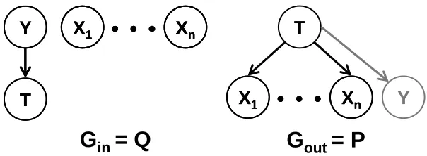
2.2 Multivariate Information Bottleneck

The information bottleneck method (Tishby et al., 1999) is a general non-parametric information-theoretic clustering framework. Given a joint distribution Q(Y,X)of two variables, it attempts to extract the relevant information that Y contains about X . We can think of such information extraction as partitioning the possible values of Y into coarser distinctions that are still informative about X . (The actual details are more complex, as we shall see shortly). For example, we might want to partition the words (Y ) appearing in several documents in a way that is most relevant to the topics (X ) of these documents.

To achieve this goal, we first need a relevance measure between two random variables X and Y with respect to some probability distribution Q(X,Y). The symmetric mutual information measure (Cover and Thomas, 1991)

IIQ(X ;Y) =

∑

x,y

Q(x,y)log Q(x,y) Q(x)Q(y)

is a natural choice as it measures the average number of bits needed to convey the information X contains about Y and vice versa. It is bounded from below by zero when the variables are indepen-dent, and attains its maximum when one variable is a deterministic function of the other.

The next step is to introduce a new variable T . This variable provides the bottleneck relation between X and Y . In our words and documents example, we want T to maintain the distinctions between words (Y ) that provide information for determining the topic of a document (X ). For example, the words ’music’ and ’lyrics’ typically occur together and are typical of the same topic, and thus the distinction between them does not contribute to the prediction of the topic. At the same time, we want T to distinguish between ’music’ and ’politics’ as they correlate with markedly different topics. Formally, we define T using a stochastic function Q(T |Y). On the one hand we want T to compress Y , while on the other hand we want it to preserve information that is relevant to X . Using the mutual information defined above, a balance between these two competing goals is achieved by minimization of the Lagrangian

L

[Q] =IIQ(Y ; T)−βIIQ(T ; X), (3)

where the parameterβcontrols the tradeoff. Tishby et al. (1999) show that the optimal partition for a given value ofβsatisfies

Q(t|y) = Q(t)

Z(y,β)exp{−βID(Q(X|y)||Q(X|t))},

where

ID(P(X)||Q(X)) =

∑

x

P(x)logP(x) Q(x)

Y

T

X

₁

X

_n

Y

T

X

₁

X

_n

X

₁

X

_n

G

_in

= Q

G

_out

= P

T

X

₁

X

_n

X

₁

X

_n

Y

Figure 1: Definition of

G

in and

G

out for the multivariate information bottleneck framework.

G

in

encodes the distribution Q that compresses Y .

G

out encodes the distribution P that we

want to approximate using Q.

The multivariate extension of this framework (Friedman et al., 2001) allows us to consider the interactions of multiple observed variables using several bottleneck variables. For example, we might want to compress words (Y ) in a way that preserves information both on the topic of the document (X1) and on the author of that document (X2). In addition, there probably is a strong

correlation between the author and the topics he writes about. Evidently, the number of possible interactions may be large, and so the framework allows us to specify the interactions we desire. These interactions are represented via two Bayesian networks. The first, called

G

in, represents the

required compression, and the second, called

G

out, represents the independencies that we are striving

for between the bottleneck variables and the target variables. In Figure 1,

G

in specifies that T is a

stochastic function of its parent in the graph Y .

G

out specifies that we want T to make Y and the

variables Xi’s independent of each other.

Formally, the framework of Friedman et al. (2001), attempts to minimize the Lagrangian

L

(1)_[

_G

in,Gout] =

I

Gin−β

I

Gout,

where

I

G =

∑

i

II(Xi; PaGi )

and the information is computed with respect to the probability distribution represented by the net-work

G

. This objective is a direct generalization of Eq. (3), and as before, tractable self-consistent equations characterize the optimal partitioning. Note that, as in the basic information bottleneck formulation, the two objective of the above Lagrangian are competing. On the one hand we want to compress the information between all bottleneck variables T and their parents in

G

in. On the other

hand we want to preserve, or maximize, the information between the variables and their parents in

G

out.

Friedman et al. (2001) also present an analogous variational principal that will be useful in our framework. Briefly, the problem is reformulated as a tradeoff between compression of mutual in-formation in

G

inso that the bottleneck variable(s) T help us describe a joint distribution that follows

that form of a target Bayesian network

G

out. Formally, they attempt to minimize the following

objective function

where Q and P are joint probabilities that can be represented by the networks of

G

in and

G

out,

respectively. The two principals are analogous under the transformation β= _1+γγ and assuming

I

Gin_=II

Q(Y ; T). See Friedman et al. (2001) for more details of the relation between the two

princi-pals.

The minimization of the above Lagrangian is over possible parameterizations of Q(T |Y)(the marginal Q(Y,X)is given and fixed) and over possible parameterizations of P(Y,T,X)that can be represented by

G

out. In other words, we want to compress Y in such a way that the distribution

defined by

G

inis as close as possible to desired distribution of

G

out. The analogous principal gives

us a new view on why these two objectives are conflicting: Consider a distribution that is consistent with

G

in so that T is independent of X given Y . On the other hand, a distribution consistent with a

specific choice of

G

outmay require that X is independent of Y given T . Constructing a distribution

where both of these requirements actually hold is not useful, may results in T that is equal to either X or Y , making this bottleneck variable redundant.

The scale parameterγbalances the above two factors. Whenγis zero we are only interested in compressing the variable Y and we resort to the trivial solution of a single cluster (or an equivalent parameterization). Whenγis high we concentrate on choosing Q(T|Y)that is close to a distribution satisfying the independencies encoded by

G

out. Returning to our word-document example. We

might be willing to forgo the distinction between ’football’ and ’baseball’ in which case we would setγto a relatively low value. On the other hand, we might even want to make a minute distinction between ’Pentium’ and ’Celeron’ in which case we would setγto a high value. Obviously, there is no single correct value ofγbut rather a range of possible tradeoffs. Accordingly, several approaches were devised to explore the spectrum of solutions asγvaries. These include Deterministic annealing like approaches that start with small value ofγand progressively increase it (Friedman et al., 2001), as well as agglomerative approaches that start with a highly refined solution and gradually compress it (Slonim and Tishby, 2000, 2001; Slonim et al., 2002).

3. Information Bottleneck Expectation Maximization

The main focus of the multivariate information bottleneck (see is on distribution Q(T |Y) that is a local maxima solution of the Lagrangian This distribution can be thought of as a soft clus-tering of the original data. Our emphasis in this work is somewhat different. Given a data set

D

={x[1], . . . ,x[M]}over the observed variables X, we are interested in learning a better genera-tive model describing the distribution of the observed attributes X. That is, we want to give high probability to new data instances from the same source. In the learned network, the hidden variables will serve to summarize some part of the data while retaining the relevant information on (some) of the observed variables X.

3.1 The Information Bottleneck EM Lagrangian

If we were only interested in the training data and the cardinality of the hidden variable allows it, each state of the hidden variable would have been assigned to a different instance. Consider, for example, a variable T with|T|states that defines a soft clustering on the specific identity of words (Y ) appearing in documents while preserving the information relevant to the topic (X ) of these documents. Now suppose we are given a set of instances

D

={word[i],topic[i]} where i goes from 1 to M, the number of instances. If|T|=M then we could simply deterministically set Q(T=i|word[i]) =1 and then predict topic[i]perfectly. While this model achieves perfect training performance, it will clearly have no generalization abilities. Since we are also interested in unknown future samples, we intuitively require that the learned model “forget” the specifics of the training examples. However, in doing so we will also deteriorate the (previously deterministic) prediction of the observed variables. Thus, there is a tradeoff between the compression of the identity of specific instances and the preservation of the information relevant to the observed variables.

We now formalize this idea for the task of learning a generative model over the variables X and the hidden variable T . We define an additional variable Y to be the instance identity in the training data

D

. That is, Y takes values in{1, . . . ,M}and Y[m] =m. We define Q(Y,X)to be the empirical distribution of the variables X in the data, augmented with the distribution of the new variable Y . For each instance y, x[y]are the values X take in the specific instance. We now apply the information bottleneck framework with the graph

G

inof Figure 1. The choice of the graph

G

outdepends on the

network model that we want to learn. We take it to be the target Bayesian network, augmented by the additional variable Y , where we set T as Y ’s parent. For simplicity, we consider as a running example the simple clustering model of

G

out where T is the parent of X1, . . . ,Xn. In practice, and

as we show in Section 6 any choice of

G

outcan be used. We now want to optimize the Bottleneck

objective as defined by these two networks. This will attempt to define a conditional probability Q(T |Y)so that Q(T,Y,X) =Q(T|Y)Q(Y,X)can be approximated by a distribution that factorizes according to

G

out. This construction will aim to find T that captures the relevant information the

instance identity has about the observed attributes. The following proposition concretely defines the objective function for the particular choice of

G

inand

G

out we are dealing with.

Proposition 1

Let

1. Y be the instance identity as defined above;

2.

G

inbe a Bayesian network structure such that such that T is independent of X given Y ; and

3.

G

out be a Bayesian network structure such that Y is a leaf with T as its only parent.

Then, minimizing the information bottleneck objective function in Eq. (4) is equivalent to minimizing the Lagrangian

L

EM=IIQ(T ;Y)−γ(IEQ[log P(X,T)]−IEQ[log Q(T)]),

as a function of Q(T|Y)and P(X,T).

Note that once the above conditions are satisfied, we can still arbitrarily choose the structure of

Proof: Using the chain rule and the fact that Y and X are independent given T in

G

out), we can

write P(Y,X,T) =P(Y |T)P(X,T). Similarly, using the chain rule and the fact that X and T are independent given Y in

G

in, we can write Q(Y,X,T) =Q(Y |T)Q(T)Q(X|Y). Thus,

ID(Q(Y,X,T)||P(Y,X,T)) = IEQ

logQ(Y |T)Q(T)Q(X|Y) P(Y |T)P(X,T)

= ID(Q(Y |T)||P(Y |T)) +IEQ[log Q(X|Y)] +IEQ[log Q(T)] −IEQ[log P(X,T)].

By setting P(Y |T) =Q(Y |T), the first term reaches zero, its minimal value. The second term is a constant since we cannot change the input distribution Q(X|Y). Thus, we need to minimize the last two terms and the result follows immediately.

An immediate question is how this target function relates to standard maximum likelihood learn-ing. To explore the connection, we use a formulation of EM introduced by Neal and Hinton (1998). Although EM is usually thought of in terms of changing the parameters of the target function P, Neal and Hinton show how to view it as a dual optimization of P and an auxiliary distribution Q. This auxiliary distribution replaces the given empirical distribution Q(X)with a completed empir-ical distribution Q(X,T). Using our notation in the above discussion, we can write the functional defined by Neal and Hinton as

F

[Q,P] =IEQ[log P(X,T)] +IHQ(T |Y), (5)

whereIHQ(T |Y) =IEQ[−log Q(T |Y)], and Q(X,Y)is fixed to be the observed empirical

distribu-tion.

Theorem 2 (Neal and Hinton, 1998) If(Q∗,P∗)is a stationary point of

F

, then P∗ is a stationary point of the log-likelihood functionIEQ[log P(X)].

Moreover, Neal and Hinton show that an EM iteration corresponds to maximizing

F

[Q,P]with respect to Q(T |Y) while holding P fixed, and then maximizing

F

[Q,P]with respect to P while holding Q(T |Y)fixed. The form of

F

[Q,P]is quite similar to the IB-EM Lagrangian, and indeed we can relate the two.

Theorem 3

L

EM= (1−γ)IIQ(T ;Y)−γ

F

[Q,P].

Proof: Plugging the identityIHQ(T |Y) =−IEQ[log Q(T)]−IIQ(T ;Y) into the EM functional we

can write

F

[Q,P] =IEQ[log P(X,T)]−IEQ[log Q(T)]−IIQ(T ;Y).

If we now multiply this byγ, and re-arrange terms, we get the form of Proposition 1.

the Lagrangian and the EM functional coincide and finding a local minimum of

L

EM is equivalent to finding a local maximum of the likelihood function. Slonim and Weiss (2002) provide a similar result for the specific case where the generative model is a mixture model of a univariate X . Their formulation is different than ours in several subtle details that do not allow a direct relation between the two methods. Nonetheless, both Slonim and Weiss (2002) and Theorem 3 show that for a par-ticular value ofγ, the information bottleneck Lagrangian coincides with the likelihood objective of EM. The main difference between the two results is the choice of generative models, in our case general multi-variate Bayesian networks, and in the case of Slonim and Weiss (2002), univariate mixture models.

3.2 The Information Bottleneck EM Algorithm

Using the above results, we can now describe the Information Bottleneck EM algorithm given a specific value of γ. The algorithm can be described similarly to the EM iterations of Neal and Hinton (1998).

• E-step: Maximize−

L

EMby varying Q(T |Y)while holding P fixed.

• M-step: Maximize−

L

EMby varying P while holding Q fixed.

Note that the algorithm is formulated in terms of maximizing−

L

EMrather than minimizing

L

EMto enhance the relation between the Lagrangian and the EM objective.

The M-Step is essentially the standard maximum likelihood optimization of Bayesian networks. To see that, note that the only term that involves P isIEQ[log P(X,T)]. This term has the form of a

log-likelihood function, where Q plays the role of the empirical distribution. Since the distribution is over all the variables, we can use sufficient statistics of P for efficient estimates, just as in the case of complete data. Thus, the M step consists of computing expected sufficient statistics given Q, and then using a closed form formula for choosing the parameters of P.

The E-step is a bit more involved. We need to maximize with respect to Q(T |Y). To do this we use the following two results that are variants of Theorem 7.1 and Theorem 8.1 of Friedman et al. (2001) and proved using similar techniques (see Appendix A for the full proof).

Proposition 4 Let

L

EM be defined via

G

in and

G

out as in Proposition 1. Q(T |Y) is a stationary

point of

L

EM with respect to a fixed choice of P if and only if for all values t and y of T and Y ,

respectively,

Q(t|y) = 1

Z(y,γ)Q(t)

1−γ_P(x[y],t])γ_{, (6)}

where Z(y,γ)is a normalizing constant:

Z(y,γ) =

∑

t0

Q(t0)1−γ_P(x[y],t0_])γ_.

Note that, as can be expected from Theorem 3, whenγ=1 the update equation reduces to Q(t|y)∝

P(x[y],t)which is equivalent to the standard EM update equation.

Proposition 5 A stationary point of

L

EMis achieved by iteratively applying the self-consistent

Combining this result with the result of Neal and Hinton that show that optimization of P increases F(P,Q), we conclude that both the E-step and the M-step increase−

L

EMuntil we reach a stationary point. As in standard EM, in most cases the stationary convergence point reached by applying these self-consistent equations will be a local maximum of−

L

EM, or a local minimum of

L

EM.

4. Bypassing Local Maxima using Continuation

As discussed in the previous section, the parameter γ balances between compression of the data and the fit of parameters to

G

out. When γ is close to 0, our only objective is compressing the

data and the effective dimensionality of T will be 1, leading to a trivial solution (or an equivalent parameterization). At larger values ofγwe pay more and more attention to the distribution of

G

out,

and we can expect additional states of T to be utilized. Ultimately, we can expect each sample to be assigned to a different cluster (if the dimensionality of T allows it), in which case there is no compression of Y and the information about the X s is fully preserved. Theorem 3 also tells us that at the limit ofγ=1 our solution will actually converge to one of the standard EM solutions. In this section we show how to utilize the inherent tradeoff determined byγto bypass local maxima towards a better solution atγ=1.

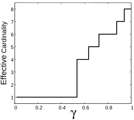
Naively, we could allow a large cardinality for the hidden variable, setγto a high value and find the solution of the bottleneck problem. There are several drawbacks to this approach. First, we will typically converge to a sub-optimal solution for the given cardinality andγ, all the more so forγ=1 where there are many such maxima. Second, we often do not know the cardinality that should be assigned to the hidden variable. If we use a cardinality for T that is too large, learning will be less robust and might become intractable. If T has too low a dimensionality, we will not fully utilize the potential of the hidden variable. We would like to somehow identify the beneficial number of clusters without having to simply try many options.

To cope with this task, we adopt the deterministic annealing strategy (Rose, 1998). In this strategy, we start withγ=0 where a single cluster solution is optimal and compression is total. We then progress toward higher values ofγ. This gradually introduces additional structure into the learned model. Intuitively, the algorithm starts at a place where a single, easy to compute solution exists, and tracks it through various stages of progressively complex solutions hopefully bypassing local maxima by staying close to the optimal solution at each value ofγ. There are several ways of executing this general strategy. The common approach is simply to increase γin fixed steps, and after each increment apply the iterative algorithm to re-attain a (local) maxima with the new value ofγ. On the problems we examine in Section 6, this naive approach did not prove successful.

0

1

L

E

M

γγγγ

Q

easy

EM

L

E

M

γγγγ

Q

0

1

∇

∇

∇

∇

G

γγγγ

Q

0

1

∆∆∆∆

(a) (b) (c)

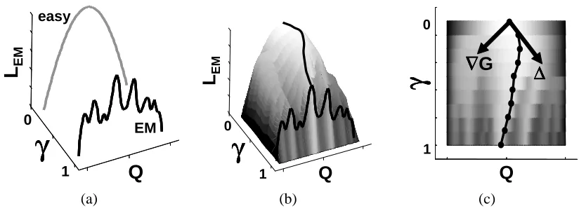
Figure 2: Synthetic illustration of the continuation process. (a) shows the easy likelihood function atγ=0 and the complex EM function atγ=1. (b) spans the full range of functions and marks the desired path for following the maximum. (c) demonstrates a single step in the continuation process. The gradient∇Q,γG is computed and then the orthogonal direction is taken.

We start by characterizing such paths. Note that once we fix the parameters Q(T|Y), the M-step maximization of the parameters in P is fully determined as a function of Q. Thus, we take Q(T|Y) andγas the only free parameters in our problem. As we have shown in Proposition 4, when the gradient of the Lagrangian is zero, Eq. (6) holds for each value of t and y. Thus, we want to consider paths where all of these equations hold. Rearranging terms and taking a log of Eq. (6) we define

Gt,y(Q,γ) =−log Q(t|y) + (1−γ)log Q(t) +γlog P(x[y],y)−log Z(y,γ). (7)

Clearly, Gt,y(Q,γ) =0 exactly when Eq. (6) holds for all t and y. Our goal is then to follow an

equi-potential path where all Gt,y(Q,γ)functions are zero starting from some small value ofγup to

the desired EM solution atγ=1.

Suppose we are at a point(Q0,γ0), where Gt,y(Q0,γ0) =0 for all t and y. We want to move in a

direction∆= (dQ,dγ)so that(Q0+dQ,γ0+dγ)also satisfies the fixed point equations. To do so,

we want to find a direction∆, so that

∀t,y, ∇Q,γGt,y(Q0,γ0)·∆=0, (8)

where∇Q,γGt,y(Q0,γ0)is the gradient of Gt,y(Q0,γ0)with respect to the parameters Q andγ.

Com-puting these derivatives with respect to each of the parameters results in a derivative matrix

Ht,y(Q,γ) =

_∂G

t,y(Q,γ))

∂Q(t|y)

∂Gt,y(Q,γ)

∂γ

. (9)

To find a direction∆that satisfies Eq. (8) we need to satisfy the matrix equation

Ht,y(Q0,γ0)∆=0. (10)

In other words, we are trying to find a vector in the null-space of Ht,y(Q0,γ0)(Q0,γ0). The matrix H

is an L×(L+1)matrix and its null-space is defined by the intersection of L tangent planes, and is of dimension L+1−Rank(Ht,y(Q,γ)). Numerically, excluding measure zero cases (Watson, 2000),

we expect Rank(Ht,y(Q0,γ0))to be full, i.e., L. Thus, a unique line that (up to scaling) defines the

null space, and we can choose any vector along it. To follow the path to our target objective at

γ=1 we choose the direction that always increasesγ(we discuss the choice of the length of this vector below). Returning to Figure 2, (c) illustrates this process. Shown is joint(γ,Q)-space with the grey-level denoting the value of the likelihood function. At each point in the learning process the gradient of G is evaluated and the orthogonal direction is taken to follow the desired path.

Finding this direction, however, can be costly. Notice that Ht,y(Q,γ)is of size L(L+1). This

number is quadratic in the training set size, and full computation of the matrix is impractical even for small data sets. Instead, we resort to approximating Ht,y(Q,γ)by a matrix that contains only

the diagonal entries ∂Gt,y(Q,γ)

∂Q(t|y) and the last column

∂Gt,y(Q,γ)

∂γ . While we cannot bound the extent of this diagonal approximation, we note that the diagonal terms are also the most significant ones and many off diagonal terms are zero. Once we make the approximation, we can solve Eq. (10) in time linear in L. (See Appendix B for a full development of H and the computation of the orthogonal direction. )

Note that once we find a vector∆that satisfies Eq. (10), we still need to decide on its length, or the size of the step we want to take in that direction. There are various standard approaches, such as normalizing the direction vector to a predetermined size. However, in our problem, we have a natural measure of progress that stems from the tradeoff defined by the target Lagrangian

L

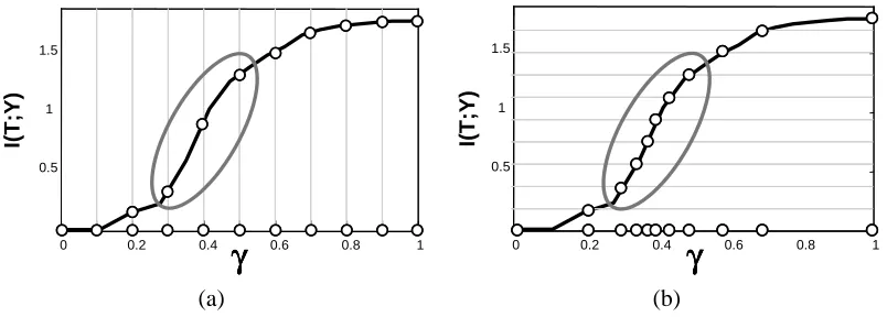
EM , whereII(T ;Y)increases when T captures more and more information about the samples during the annealing procedure. That is, the “interesting” steps in the learning process occur when II(T ;Y) grows. These are exactly the points where the balance between the two terms in the Lagrangian changes and the second term grows sufficiently to allow the first term to increaseII(T ;Y). Using II(T ;Y)to gauge the progress of the annealing procedure is appealing since it is a non-parametric measure that does not involve the form of the particular distribution of interest P. In addition, in all runsII(T ;Y)starts at 0, and is upper-bounded by the log of the cardinality of T and we are thus given a scale of progress.

With this intuition at hand, we want to normalize the step size by the expected change inII(T ;Y). That is, we calibrate our progress with respect to the actual amount of regularization applied at the current value ofγ. At regions where II(T ;Y)is not sensitive to changes in the parameters, we can proceed rapidly. On the other hand, if small changes in the parameters result in significant changes ofII(T ;Y), then we want to carefully track the solution. Figure 3 illustrates the difference between using a predetermined step of γand partitioningII(T ;Y) in order to determine the step size. It is evident the usingII(T ;Y)causes the method to concentrate on the region of interest in terms of rapid change of the Lagrangian.

Formally, we compute∇Q,γII(T ;Y)and rescale the direction vector so that

γγγγ

0 0.2 0.4 0.6 0.8 1

0.5 1 1.5

I(

T

;Y

)

γγγγ

0 0.2 0.4 0.6 0.8 1

0.5 1 1.5

I(

T

;Y

)

(a) (b)

Figure 3: Illustration of the step size calibration process. Both graphs show the change in informa-tion between T and Y as a funcinforma-tion ofγ. The circles denote values ofγto be evaluated. (a) shows naive calibration when fixed steps are taken in theγrange. (b) shows calibra-tion that uses fixed steps in the informacalibra-tion range. The grey circle shows the region of dramatic change of the Lagrangian.

whereεis a predetermined step size that is a fraction of log|T|. We also bound the minimal and maximal change inγso that we do not get trapped in too many steps or alternatively overlook the regions of change.

Finally, although the continuation method takes us in the correct direction, the approximation as well as inherent numerical instability can lead us to a suboptimal path. To cope with this situation, we adopt a commonly used heuristic used in deterministic annealing. At each value ofγ, we slightly perturb the current solution and re-iterate the self-consistent equations to converge on a solution. If the perturbation leads to a better value of the Lagrangian, we take it as our current solution.

To summarize, our procedure works as follows: we start with γ=0 for which only trivial solutions exists. At each stage we compute the joint direction ofγand Q(T |Y)that will leave the fixed point equations intact. We then take a small step in this direction and apply IB-EM iterations to attain the fixed point equilibrium at the new value ofγ. We repeat these iterations until we reach

γ=1.

5. Multiple Hidden Variables

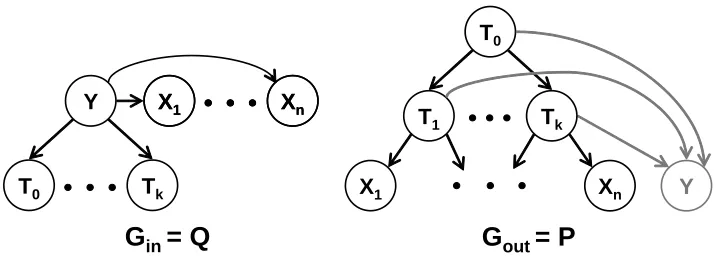
The framework we described in the previous sections can easily accommodate learning networks with multiple hidden variables simply by treating T as a vector of hidden variables. In this case, the distribution Q(T|Y)describes the joint distribution of the hidden variables for each value of Y , and P(T,X)describes their joint distribution with the attributes X in the desired network. Unfortunately, if the number of variables T is large, the representation of Q(T|Y)grows exponentially, and this approach becomes infeasible.

One strategy to alleviate this problem is to force Q(T|Y)to have a factorized form. This reduces the cost of representing Q and also the cost of performing inference. As an example, we can require that Q(T|Y) is factored as a product ∏iQ(Ti |Y). This assumption is similar to the mean field

G

_in

= Q

X₁ X_n

X₁ X_n

Y

T₀ T_k

G

_out

= P

X₁ X_n Y

T₀

T₁ T_k

Figure 4: Definition of networks for the multivariate information bottleneck framework with mul-tiple hidden variables. Shown are

G

in with the mean field assumption, and a possible

choice for

G

out.

In the multivariate information bottleneck framework, different factorizations of Q(T|Y) cor-respond to different choices of networks

G

in. For example, the mean field factorization is achieved

when

G

in is such that the only parent of each Ti is Y , as in Figure 4. In general, we can consider

other choices where we introduce edges between the different Ti’s. For any such choice of

G

in, we

get exactly the same Lagrangian as in the case of a single hidden variable. The main difference is that since Q has a factorized form, we can decomposeIIQ(T;Y). For example, if we use the mean

field factorization, we get

IIQ(T;Y) =

∑

i

IIQ(Ti;Y).

Similarly, we can decomposeIEQ[log P(X,T)]into a sum of terms, one for each family in P. These

two factorization can lead to tractable computation of the first two terms of the Lagrangian as written in Proposition 1. Unfortunately, the last termIEQ[log Q(T)]cannot be evaluated efficiently. Thus, we

approximate this term as∑iIEQ[log Q(Ti)]. For the mean field factorization, the resulting Lagrangian

(with this lower bound approximation) has the form

L

EM+ =

∑

i

IIQ(Ti;Y)−γ IEQ[log P(X,T)]−

∑

i

IEQ[log Q(Ti)]

!

. (12)

The form of

L

EM+ is valid, if Proposition 1 still holds for the case of multiple hidden variables. This is immediate if we make the following requirements, similar to those made for the case of a single hidden variable:

1. Y is the instance identity;

2.

G

inis a Bayesian network structure such that all of the variables T are independent of X given

Y ; and

3.

G

outis a Bayesian network structure such that Y is a child of T and has no other parents. This

The last requirement is needed so that we can set P(Y |T) =Q(Y |T)in the proof of Proposition 1. As in the case of a single hidden variable, we can now characterize fixed point equations that hold in stationary points of the Lagrangian.

Proposition 6 Let

L

EM+ be defined via

G

in and

G

out as in Eq. (12). Assuming a mean field

approxi-mation for Q(T|Y), a (local) maximum of

L

EM+ is achieved by iteratively solving, independently for

each hidden variable i, the self-consistent equations

Q(ti|y) =

1

Z(i,y,γ)Q(ti)

1−γ_exp{γEP(t i,y)},

where

EP(ti,y)≡IE_Q(T|ti,y)[log P(x[y],T)]

and Z(i,y,γ)is a normalizing constant that equals to

Z(i,y,γ) =

∑

t0

i

Q(t_i0)1−γexpγEP t_i0,y .

See Appendix A for the proof.

The only difference from the case of a single hidden variables is in the form of the expecta-tion EP(ti,y). It is easy to see that when a single hidden variable is considered, and EP(ti,y)≡

log P(x[y],t), the two forms coincide. It is also easy to see that this term decomposes into a sum of expectations, one for each factor in the factorization of P. We note that only terms that average over factors that involve Ti are of interest in EP(ti,y). All other terms do not depend on the value of Ti,

and can be absorbed by the normalizing constant. Thus, EP(ti,y)can still be computed efficiently.

A more interesting consequence (see theorem below) of this discussion is that when γ=1, maximizing

L

EM+ is equivalent to performing mean field EM (Jordan et al., 1998). Thus, by using the modified Lagrangian we generalize this variational learning principle, and as we show below manage to reach better solutions.

The formulation is easily extensible to a general variational approximation of Q where

G

in

allows, in addition to the dependence of each Ti on Y , dependencies between the different Ti’s. In

this case, we get

IIQ(T;Y) =

∑

i

IIQ(Ti; PaG_i in).

Similarly,IEQ[log P(X,T)]decomposes according to the joint families of Tiin P and in Q. That is,

each term in the decomposition depends on Ti, its parents PaGiinin

G

in, and its parents PaGiout in

G

out.

As in the case of the mean field variational approximation, the last termIEQ[log Q(T)]cannot be

evaluated efficiently. We approximate it using a decomposition that follows the structure of

G

inas

IEQ[log Q(T)]≈

∑

i

IEQ

h

log Q(Ti|T∩Pa

Gin

i )

i

. (13)

We can now reformulate the results of Theorem 3 for this general case:

Theorem 7 Let Q(T|Y)decompose according to any structure

G

inwhere all Ti’s are descendents

of Y and replaceIEQ[log Q(T)]by a decomposition as defined in Eq. (13). Then for the resulting

Lagrangian

L

EM+ = (1−γ)

∑

i

IIQ(Ti; Pa

Gin

i )−γ

F

0 20 40 60 80 100

-435.5 -434.5 -433.5

Percentage of random runs

T

e

s

t

L

L

/

i

n

s

ta

n

c

e

mean field EM ~2.6 hours single IB-EM ~85 hours

each exact EM > 17 hours

(a) (b)

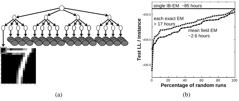
Figure 5: (a) A quadrant based hierarchy structure with 21 hidden variables for modeling 16×16 images in theDigitdomain. (b) Test log-loss of the IB-EM algorithm for the model of (a) compared to the cumulative performance of 50 random EM and mean field EM runs.

where

F

+[Q,P]is defined as in Eq. (5), except that the above decomposition for bothIEQ[log P(X,T)]

andIHQ(T|Y)is used.

Proof: This is a direct result of the fact that in the proof of Theorem 3, no assumptions were made of the form of Q.

The above theorem extends the formal relation of the information bottleneck target Lagrangian and the EM functional for any form of variational approximation encoded by

G

in. In particular, when

γ=1, finding a local minimum of

L

EM+ is equivalent to finding a local maximum of the likelihood function when the same variational approximation is used in the EM algorithm. Similarly, we can derive the fixed point equations with each for different choices of

G

in. The change to Proposition 6

is simply a different decomposition for EP(i,y)

To summarize, the IB-EM algorithm of Section 3.2 can be easily generalized to handle multiple hidden variables by simply altering the form of EP(ti,y) in the fixed point equations. All other

details, such as the continuation method, remain unchanged.

6. Experimental Validation: Parameter Learning

To evaluate the IB-EM method for the task of parameter learning, we examine its generalization performance on several types of models on three real-life data sets. In each architecture, we consider networks with hidden variables of different cardinality, where for now we use the same cardinality for all hidden variables in the same network. We now briefly describe the data sets and the model architectures we use.

• TheDigitsdata set contains 7291 training instances and 2007 test instances from the USPS (US Postal Service) data set of handwritten digits (see http://www.kernel-machines.org/data.html). An image is represented by 256 variables, each denoting the gray level of one pixel in a 16×16 matrix. We discretized pixel values into 10 equal bins.

On this data set we tried several network architectures. The first is a Naive Bayes model with a single hidden variable. In addition, we examined more complex hierarchical models. In these models we introduce a hidden parent to each quadrant of the image recursively. The 3-level hierarchy has a hidden parent to each 8x8 quadrant, and then another hidden variable that is the parent of these four hidden variables. The 4-level hierarchy starts with 4x4 pixel blocks each with a hidden parent. Every 4 of these are joined into an 8x8 quadrant by another level of hidden variables, totaling 21 hidden variables, as illustrated in Figure 5(a).

• TheYeastdata set contains measurements of the expression of the Baker’s yeast genes in 173 experiments (Gasch et al., 2000). These experiments measure the yeast response to changes in its environmental conditions. For each experiment the expression of 6152 genes were measured. We discretized the expression levels of genes into ranges down/same/up by using a threshold of one standard deviation from above and below the gene’s mean expression across all experiments. In this data set, we treat each gene as an instance that is described by its behavior in the different experiments. We randomly partitioned the data into 4922 training instances (genes) and 1230 test instances.

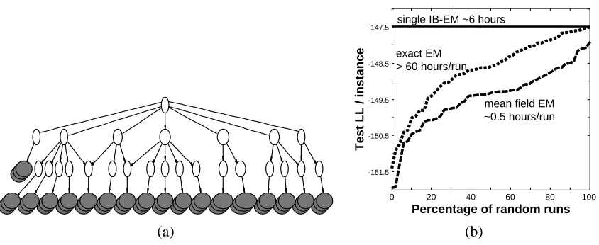
The model we use for this data set has an hierarchical structure with 19 hidden variables in a 4-level hierarchy that was determined by the biological expert based on the nature of the different experiments, as illustrated schematically in Figure 6. In this structure, 5–24 similar conditions (filled nodes) such as different hypo-osmotic shocks are children of a common hidden parent (unfilled nodes). These hidden parents are in their turn children of further ab-straction of conditions. For example, the heat shock and heat shock with oxidative stress hidden nodes, are both children of a common more abstract heat node. A root hidden vari-able is the common parents of these high-level abstractions. Intuitively, each hidden varivari-able encodes how the specific instance (a gene) is altered in the relevant groups of conditions.

As a first sanity check, for each model (and each cardinality of hidden variables) we performed 50 runs of EM with random starting points. The parameter sets learned in these different runs have a wide range of likelihoods both on the training set and the test set. These results (on which we elaborate below), indicate that these learning problems are challenging in the sense that EM runs can be trapped in markedly different local maxima.

mean field EM ~0.5 hours/run single IB-EM ~6 hours

exact EM > 60 hours/run

-151.5 -150.5 -149.5 -148.5 -147.5

0 20 40 60 80 100

Percentage of random runs

T

e

s

t

L

L

/

i

n

s

ta

n

c

e

(a) (b)

Figure 6: (a) A structure constructed by the biological expert for theYeastdata set based on prop-erties of different experiments. 5-24 similar conditions (filled nodes) are aggregated by a common hidden parent (unfilled nodes). These hidden nodes are themselves children of further abstraction nodes of similar experiments, which in their turn are children of the single root node. (b) Comparison of test performance when learning the parameters of the structure of (a) with binary variables. Shown is test log-likelihood per instance of the IB-EM algorithm and the cumulative performance of 50 random EM as well as 50 random mean field EM runs.

It is important to note the time required by these runs, all on a Pentium IV 2.4 GHz machine. For theDigitdata set, a single mean field EM run requires approximately 2.5 hours, an exact EM run requires roughly 17 hours, and the single IB-EM run requires just over 85 hours. As the IB-EM run reaches a solution that is better than all of this runs, it offers an appealing performance to time tradeoff. This is even more evident for the Yeastdata set where the structure is somewhat more complex and the difference between exact learning and the mean field approximation is greater. For this data set, the single IB-EM is still superior and takes significantly less time than a single exact EM.

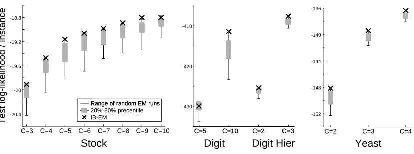
Figure 7 compares the test log-likelihood per instance performance of our IB-EM algorithms and 50 random EM runs for a range of models for theStock, Digit andYeast data sets. In most cases, IB-EM is better than 80% of the EM runs and is often as good or better than the best of them. The advantage of IB-EM is particularly pronounced for the more complex models with higher cardinalities. Table 1 provides more details of these runs including train performance and comparison to 50 random mean field EM runs.

L

E

A

R

N

IN

G

H

ID

D

E

N

V

A

R

IA

B

L

E

N

E

T

W

O

R

K

S

Stock

C=3 -19.91 62% -19.90 -19.90 -19.90 76% -19.88 -19.89

C=4 -19.47 98% -19.46 -19.52 -19.52 96% -19.52 -19.62

C=5 -19.16 94% -19.15 -19.24 -19.31 98% -19.30 -19.39

Digit

C=5 -429.95 36% -428.67 -429.11 -439.91 56% -439.03 -439.47 C=10 -411.44 100% -411.72 -413.96 -425.33 100% -425.36 -427.05 DigH3

C=2 -442.02 100% -442.02 -442.29 100% -442.03 -442.20 -450.812 92% -450.76 -450.92 82% -450.76 -450.84 C=3 -428.77 100% -428.85 -429.02 100% -428.83 -429.02 -437.798 98% -437.74 -438.20 98% -437.74 -438.04 DigH4

C=2 -425.43 100% -425.54 -425.81 100% -425.61 -425.94 -433.279 100% -433.30 -433.55 100% -433.40 -433.71 C=3 -407.60 100% -407.75 -408.56 100% -408.49 -408.83 -415.798 100% -415.88 -416.48 100% -416.37 -416.77 Yeast

C=2 -148.13 100% -148.32 -148.79 100% -148.89 -149.71 -147.48 100% -147.51 -147.87 100% -147.92 -148.78 C=3 -139.44 100% -139.58 -140.05 100% -140.09 -140.87 -138.38 100% -138.57 -139.00 100% -139.06 -139.92 C=4 -136.36 100% -136.72 -136.97 100% -137.72 -138.28 -135.65 100% -135.96 -136.16 100% -136.92 -137.34

Table 1: Comparison of the IB-EM algorithm, 50 runs of EM with random starting points, and 50 runs of mean field EM from the same random starting points. Shown are train and test log-likelihood per instance for the best and 80th percentile of the random runs. Also shown is the percentile of the runs that are worse than the IB-EM results. Data sets shown include a Naive Bayes model for the

Stockdata set and theDigitdata set; a 3 and 4 level hierarchical model for theDigitdata set (DigH3andDigH4); and an hierarchical

model for theYeastdata set. For each model we show several cardinalities for the hidden variables, shown in the first column.

1

0

T

e

s

t

lo

g

-l

ik

e

lih

o

o

d

/

i

n

s

ta

n

c

e

Stock

C=3 C=4 C=5 C=6 C=7 C=8 C=9 C=10

-20.4 -20 -19.6 -19.2 -18.8

Range of random EM runs Range of random EM runs 20%-80% precentile IB-EM

Digit Digit Hier

C=5 C=10

C=5 C=10 C=2C=2 C=3C=3

-430 -420 -410

Yeast

C=2 C=3 C=4

-152 -148 -144 -140 -136

Figure 7: Comparison of log-likelihood per instance test performance of the IB-EM algorithm (black ’X’) and 50 runs of EM with random starting points. The vertical line shows the range of the random runs and boxes mark the 20%-80% range. Data sets shown (x-axis) include a Naive Bayes model for theStockdata set and theDigitdata set; a 4 level hierarchical model for the Digitdata set (Digit Hier); a hierarchical model for theYeast data set. For each model we show several cardinalities for the hidden variables, shown in the x-axis.

efficient parameter settings, the perturbation method’s performance was significantly inferior to that of IB-EM. These results do not contradict those of Elidan et al. (2002) who showed some improvement for the case of parameter learning but mainly focused on structure learning, with and without hidden variables.

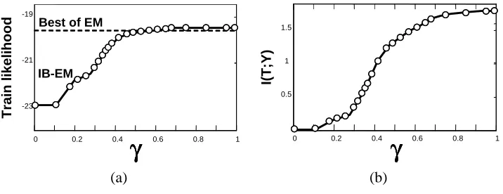
To demonstrate the effectiveness of the continuation method we examine IB-EM during the progress ofγ. Figure 8 illustrates the progression of the algorithm on theStockdata set. (a) shows training log-likelihood per instance of parameters in intermediate points in the process. This panel also shows the values ofγevaluated during the continuation process (circles). These were evaluated using the predicted change inII(T ;Y)shown in (b). As we can see, the continuation procedure fo-cuses on the region where there are significant changes inII(T ;Y)approximately corresponding the areas of significant changes in the likelihood. For both theStockandDigitdata sets, we also tried changingγnaively from 0 to 1 as in standard annealing procedures, without performing continua-tion. This procedure often “missed” the superior local maxima even when a large number (1000) of

γvalues were used in the process. In fact, in most runs the results were no better than the average random EM run emphasizing the importance of the continuation in the annealing process.

7. Learning Structure

γγγγ

0 0.2 0.4 0.6 0.8 1

-23 -21 -19

T

ra

in

l

ik

e

li

h

o

o

d

IB-EM Best of EM

0 0.2 0.4 0.6 0.8 1

0.5 1 1.5

I(

T

;Y

)

γγγγ

(a) (b)

Figure 8: The continuation process for a Naive Bayes model on theStockdata set. (a) Shows the progress of training likelihood as a function ofγcompared to the best of 50 EM random runs. Black circles illustrate the progress of the continuation procedure by denoting the value of γat the end of each continuation step. Calibration is done using information between the hidden variable T and the instance identity Y shown in (b) as a function ofγ.

parameter learning, which is just one of the tasks we have to perform in this scenario. The common approach to this model selection task is to use a score-based approach where we search for a struc-ture that maximizes some score. Common scores such as the BDe score (Heckerman et al., 1995) balance the likelihood achieved by the model and its complexity. Thus, model selection is achieved independently of the search procedure used (see Section 2.1 for more details).

We now aim to extend the IB-EM framework for the task of structure learning using a score-based approach. Naively, we could simply consider different structures and for each one apply the IB-EM procedure to estimate parameters, and then evaluate its generalization ability using the score. Such an approach is extremely inefficient, since it spends a non-trivial amount of time to evaluate each potential candidate structure. In this work we advocate a strategy that is based on the structural EM framework of Friedman (1997). In structural EM, we use the completion distribution Q that is a result of the E-Step to compute expected sufficient statistics. That is, instead of Eq. (1), we use

IEQ(T|Y)[N(xi,pai)] =

∑

m

∑

t

Q(

X

[m] =xi,Pai=pai,t|Y =m).

These statistics are then used in the M-step when structure modification steps are evaluated. Thus, instead of assuming that the target structure

G

outis fixed, we define the Lagrangian as a function of

the pair(

G

out,θ). Then, in the M-step, we can consider different choices of

G

out and evaluate how

each of them changes the score. Given the expected statistics, the problem is identical in form to learning from a fully observed data set and computation of the score is similar. This facilitates an efficient greedy search procedure that uses local edge modification to the network structure. The EM procedure of Section 3.2 is thus revised as follows:

• E-step : Maximize−

L

EMby varying Q(T |Y)while holding P fixed.