Generalization Bounds and Complexities Based on Sparsity and Clustering for Convex Combinations of Functions from Random Classes

Generalization Bounds and Complexities

Based on Sparsity and Clustering

for Convex Combinations of Functions from Random Classes

Savina Andonova Jaeger [email protected]

Harvard Medical School Harvard University Boston, MA 02115, USA

Editor: John Shawe-Taylor

Abstract

A unified approach is taken for deriving new generalization data dependent bounds for several classes of algorithms explored in the existing literature by different approaches. This unified ap-proach is based on an extension of Vapnik’s inequality for VC classes of sets to random classes of sets - that is, classes depending on the random data, invariant under permutation of the data and possessing the increasing property. Generalization bounds are derived for convex combinations of functions from random classes with certain properties. Algorithms, such as SVMs (support vec-tor machines), boosting with decision stumps, radial basis function networks, some hierarchies of kernel machines or convex combinations of indicator functions over sets with finite VC dimension, generate classifier functions that fall into the above category. We also explore the individual com-plexities of the classifiers, such as sparsity of weights and weighted variance over clusters from the convex combination introduced by Koltchinskii and Panchenko (2004), and show sparsity-type and cluster-variance-type generalization bounds for random classes.

Keywords: complexities of classifiers, generalization bounds, SVM, voting classifiers, random classes

1. Introduction

Statistical learning theory explores ways of estimating functional dependency from a given collec-tion of data. It, also referred to as the theory of finite samples, does not rely on a priori knowledge about a problem to be solved. Note that “to control the generalization in the framework of this paradigm, one has to take into account two factors, namely, the quality of approximation of given data by the chosen function and the capacity of the subset of functions from which the approxi-mating function was chosen” (Vapnik, 1998). Typical measures of the capacity of sets of functions are entropy measures, VC-dimensions and V-γdimensions. Generalization inequalities such as Vap-nik’s inequalities for VC-classes, which assert the generalization performance of learners from fixed class of functions and take into account the quality of approximation of given data by the chosen function and the capacity of the class of functions, were proven to be useful in building successful learning algorithms such as SVMs (Vapnik, 1998).

satisfies Dudley’s uniform entropy condition if Z ∞

0

log1/2D(

F

,u)du<∞,

where D(

F

,u) denotes Koltchinksii packing numbers defined for example by Dudley (1999) or Panchenko (2002). Applications of the inequality were shown in several papers (Koltchinskii and Panchenko, 2002; Koltchinskii et al., 2003a; Koltchinskii and Panchenko, 2004) which explored the generalization ability of ensemble classification methods, that is, learning algorithms that combine several classifiers into new voting classifiers with better performance. “The study of the convex hull, conv(

H

), of a given base function class

H

has become an important object of study in machine learning literature” (Koltchinskii and Panchenko, 2004). New measures of individual complexities of voting classifiers derived in related work (Koltchinskii et al., 2003a; Koltchinskii and Panchenko, 2004; Koltchinskii et al., 2003b) were shown theoretically and experimentally to play an important role in the generalization performance of the classifiers from conv(

H

)of a given base function class

H

. In order to do so, the base class

H

is assumed to have Koltchinskii packing numbers satisfying the following condition

D(

H

,u)_≤K(V)u−V,

for some V >0,and where K depends only on V . “New margin type bounds that are based to a greater extent on complexity measures of individual classifier functions from the convex hull, are more adaptive and more flexible than previously shown bounds” (Koltchinskii and Panchenko, 2004).

Here, we are interested in studying the generalization performance of functions from a convex hull of random class of functions (random convex hull), that is, the class of learners is no longer fixed and depends on the data. This is done by deriving a new version of Vapnik’s inequality applied to random classes, that is, a bound for relative deviations of frequencies from probabilities for random classes of events. The proof of the inequality mirrors the proofs of Vapnik’s inequality for non-random classes of sets (see Vapnik et al., 1974; Vapnik, 1998; Anthony and Shawe-Taylor, 1993) but with the observation that the symmetrization step of the proof can be carried out for random classes of sets. The new version of Vapnik’s inequality is then applied to derive flexible and adaptive bounds on the generalization errors of learners from random convex hulls. We exploit techniques previously used in deriving generalization bounds for convex combinations of functions from non-random classes in (Koltchinskii and Panchenko, 2004), and several measures of individual classifier complexities, such as effective dimension, pointwise variance and weighted variance over clusters, similar to the measures introduced by Koltchinskii and Panchenko (2004).

2. Definition of Random Classes

First, an inequality that concerns the uniform relative deviation over a random class of events of relative frequencies from probabilities is exhibited. This inequality is an extension of the following Vapnik’s inequality for a fixed VC-class

C

(with finite VC-dimension V ) of sets (see Vapnik et al. (1974); Vapnik (1998); Anthony and Shawe-Taylor (1993)):

Pn

sup C∈C

hP_(C)−1

n∑ n

i=1I(xi∈C)

p

(P_(C))

i

≥t

≤4

_2en

V

V

e−nt24 . (2.1)

Inequality (2.1) allows one to prove stronger generalization results for several problems dis-cussed in (Vapnik, 1998). In order to extend the above inequality to random classes of sets, we intro-duce the following definitions. Let(

Z

,

S

,P_{)be a probability space. For a sample{z1, . . . ,zn},zi∈}

Z

,i=1, . . . ,n,define zn_{= (z}

1, . . . ,zn)and let I(zn) ={zi: 1≤i≤n}.Let

C

(zn)∈

S

be a class of sets, possibly dependent on the sample zn= (z1, . . . ,zn)∈

Z

n.

The integer∆C(zn₎(zn) is defined to be the number of distinct sets of the form ATI(zn),where A runs through

C

(zn_{),that is,}∆

C(zn₎(zn) =card{AT{z₁, . . . ,z_n},A∈

C

(zn)}.The random collection of level sets

C

(zn) =nA=_{z_∈

Z

: h(z)_≤0_},h_∈

H

(z1, . . . ,zn)

o

,where

H

(zn)is a random class of functions possibly depending on znserves as a useful example. We call AT

I(zn)a representation of the sample znby the set A. ∆C(zn₎(zn)is the number of different representation of{z1, . . . ,z_n}by functions from

H

(zn).

Now consider the random collection

C

(zn)of

S

-measurable subsets of

Z

,

C

(zn) =_{A : A_∈

S

},

having the following properties:

1.)

C

(zn)_⊆

C

zn[y

,zn_∈

Z

n,y_∈

Z

(2.2) (the incremental property)

2.)

C

(z_π(1), . . . ,z_π(n))_≡

C

(z1, . . . ,zn), (2.3) for any permutationπof_{z1, . . . ,zn}(the permutation property).

The relative frequency of A_∈

C

(zn)on zn= (z1, . . . ,zn)∈

Z

nis defined to be

P_zn(A) =1

n|{i : zi∈A}|= 1 n|I(z

n₎ ∩A_|,

where_|A_|denotes the cardinality of a set A.

LetPn_{be the product measure on n copies of(}

_Z

_,

_S

_,P_{), and}E_{nthe expectation with respect to} Pn_{. Define}

3. Main Results

Given the above definitions, the following theorem holds. Theorem 1 For any t>0,

Pnn_zn_∈

_Z

n_{: sup}

A∈C(zn₎

P_(A)−P_zn(A)

p

P_(A) ≥t o

≤4G(2n)e−nt24 . (3.4)

The proof of this theorem is given in the following Section 4. Observe that if the random col-lection

C

of sets is a VC-class (Vapnik, 1998), then the inequality (3.4) is the same as Vapnik’s inequality (2.1) for VC-classes. Based on this theorem and the above definitions, several results on the generalization performance and the complexity of classifiers from random classes are exhibited below.

The following notation and definitions will be used from here on. Let(

X

,

A

)be a measurable space (space of instances) and take

Y

=_{−1,1} to be the set of labels. Let P _{be the}

probabil-ity measure on

X

×

Y

,

A

×2{−1,1} and let(Xi,Yi),i=1, . . . ,n be i.i.d random pairs in

X

×

Y

, randomly sampled with respect to the distributionP_{of a random variable(X,Y).The probability}

measure on the main sample space on which all of the random variables are defined will be denoted by P. Let

Z

=

X

×

Y

,Zi= (Xi,Yi),i=1, . . . ,n and Zn= (Z1, . . . ,Zn). We will also define several random classes of functions and show how several learning algorithms generate functions from the convex hulls of random classes.

Consider the following four problems for which bounds on the generalization errors will be shown using inequality (3.4).

Problem 1. Support vector machine (SVM) classifiers with uniformly bounded kernels. Consider any solution of an SVM algorithm f(x) =∑n

i=1λiYiK(Xi,x),where K(., .):

X

×

X

→

[0,1]is the kernel andλi ≥0. sign(f(x))is used to classify x∈

X

in class +1 or −1. Take the random function class

H

(Zn) =_{YiK(Xi,x): i=1, . . . ,n}, which depends on the random sample Zn_∈

Z

n_{.The classifier function}

f0(x) =

n

∑

i=1 λ0

iYiK(Xi,x), λ0i= λi ∑n

j=1λj

, i=1, . . . ,n

belongs to conv(

H

(Zn))and the probability of errorP_{(Y f(X)≤0) =}P_{(Y f}0_(X)≤0).

Problem 2. Classifiers, built by some two-level component based hierarchies of SVMs (Heisele et al. (2001);Andonova (2004)) or kernel-based classifiers (like the one produced by radial basis function (RBF) networks).

this form sign(f(x)),where

f(x,α,Q,w2) =

d

∑

j=1 w₂j

n

∑

i=1 αj

iYiK(QjXi,Qjx),Yi=±1,

where Qj are the projections of the instances (determining the “components”), w₂j _∈R_,αj

i ≥0.One can consider Qj _{being nonlinear transformation of the instance space, for example applying filter} functions. Let_|K(x,t)_{| ≤}1,_∀x,t_∈

X

. Consider the random function class

H

(X1, . . . ,Xn) ={±K(QjXi,Qjx): i≤n,j=1, . . . ,d},

where n is the number of training points(Xi,Yi)and d is the number of the components.

In the case of RBF networks with one hidden layer and a linear threshold, the classifier function is of the form

f(x) =

d

∑

j=1 ˆ n

∑

i=1 αi

jKσj(ci,x),

where ci,i=1, . . . ,n are centers of clusters, formed by clustering the training pointsˆ {X1, . . . ,Xn}and σj (they can depend on the training data(Xi,Yi),i=1, . . . ,n) are different widths for the Gaussian kernel, Kσj(ci,x) =e

−||ci−_σ2x||2

j _{. Consider the following random function class}

H

(Zn) =_{±K_σj(ci,x): i≤nˆ,j≤d},

where ˆn is the number of clusters, which is bounded by the number n of training points, and the cluster centers_{ci}niˆ=1depend on the training instances{Xi}ni=1.

Without loss of generality, we can consider f _∈conv(

H

(Zn))in both of the above described algorithms, after normalizing the classifier function with the sum of the absolute values of the coef-ficients in front of the random functions.

Problem 3. Boosting over decision stumps.

Given a finite set of d functions _{hi:

X

×

X

→[−1,1]} for i≤d, define the random class of as

H

(X1, . . . ,Xn) ={hi(Xj,x): j≤n,i≤d},where n is the number of training points(Xi,Yi). This type of random class is used for example in aggregating combined classifier by boosting over decision stumps. Indeed, decision stumps are simple classifiers, h, of the types 2I(xi _≤a)₋1 or 2I(xi _≥a)₋1, where i_{∈ {}1, . . . ,m_} is the direction of splitting (X _⊂Rm_{) and a∈}R _{is the}

threshold. It is clear that the threshold a can be chosen among X₁i, . . . ,X_ni (the performance of the stump will remain the same on the training data). In this case, take hi(Xj,x) =2I(xi≤Xij)−1 or

e

hi(Xj,x) =2I(xi≥Xi_j)−1 and

H

(X1, . . . ,Xn) ={hi(Xj,x),ehi(Xj,x): j≤n,i≤m}and take d=2m. Without loss of generality, we can consider f _∈conv(

H

(X1, . . . ,Xn)), after normalizing with the sum of the absolute values of the coefficients.

Problem 4. VC-classes of sets.

Let the random class of functions

H

(Zn)has the property that for all h_∈

H

(Zn),h_{∈ {−}1,1_} the VC dimension V of the class of sets_{{x_∈

X

: h(x) =1_},h_∈

H

(Zn)_}is finite.

before with the previously existing VC-inequalities for indicator functions (Vapnik, 1998; Vapnik et al., 1968). The results shown here for Problem 4 in the case when

H

is a random class, are comparable to those derived before for indicators over class of sets with finite VC dimension.

In general, all of the above four types of problems, consider the convex combinations of func-tions from the random convex hull

F

(Zn) =conv(

H

(Zn)) = [ T∈N

F

T(Zn),

F

T(Zn) =

ΣT

i=1λihi,λi≥0,ΣTi=1λi=1,hi∈

H

(Zn) , (3.5) where

H

(Zn)is for example one of the random classes defined above, such that either_|

H

(Zn)_|=

card(

H

(Zn))is finite, or

H

(Zn)is a collection of indicators over random class of sets with finite VC-dimension.

General problem:

We are interested is the following general problem:

Let

H

be a general-base class of uniformly bounded functions with values in [₋1,1]. Let Z1, . . . ,Zn,Zi= (Xi,Yi)∈

X

×

Y

be i.i.d. (training data) sampled with respect to the distribution

P_{.Assume that based on the data Z1, . . . ,Zn one selects a class of functions}

_H

_(Zn_)⊆

_H

_{that is}

either

i) with finite cardinality depending on the data, such that ln(sup_Zn|H(Zn₎

|)ln n

n →0 for n→∞,or

ii)

H

(Zn)_⊆

H

is a collection of indicator functions_{2IC−1 : C∈

C

Zn}over a class of sets

C

_Zn with finite VC-dimension V .

We will call

H

(Zn)a random-base class of functions. We are interested in studying the gen-eralization errors for classifier functions f _∈conv(

H

(Zn))that are produced by broad classes of algorithms. Let us take

G∗(n,

H

) = sup Zn_∈(X×Y)n|

H

(Zn)_|,

when

H

is the general-base class and the random-base classes

H

(Zn) are with finite cardinality H(Zn), and take

G∗(n,

H

) =ne

V

V

,

when

H

is the general-base and the random-base classes

H

(Zn)are collections of indicators over class of sets with finite VC-dimension V (Problem 4).

From the definitions and Problems 1, 2 and 3, it is clear that G∗(n,

H

)_≤2n for Problem 1 and G∗(n,

H

)_≤2nd for Problems 2 and 3. For completeness of the results in case of

H

(Zn)being a collection of indicators over class of sets with finite VC-dimension V , we will assume that n_≥2eV.

Following the notation by Koltchinskii and Panchenko (2004), let

P

(

H

(Zn))be the collection of all discrete distributions over the random-base class

H

(Zn). Let λ_∈

P

(

H

(Zn)) and f(x) =

R

h(x)λ(dh),which is equivalent to f _∈conv(

H

(Zn)).The generalization error of any classifier function is defined as

Given an i.i.d sample(Xi,Yi),i=1, . . .n from the distributionP, letPn denote the empirical distri-bution and for any measurable function g on

X

×

Y

,let

P_g=

Z

g(x,y)dP_(x,y), P_ng=1

n n

∑

i=1

g(Xi,Yi).

The first bound we show for the generalization errors of functions from random classes of functions is the following:

Theorem 2 Let

H

be a general-base class of functions. For any t>0, with probability at least 1₋e−t, for any n i.i.d. random pairs (X1,Y1), . . . ,(Xn,Yn) randomly drawn with respect to the distributionP_{, for all}λ_∈

_P

₍

_H

_(Zn_{))and f(x) =}R

h(x)λ(dh),

P_{(y f(x)≤0)≤ inf}

0<δ≤1

U12+ (P_n(y f(x)≤2δ) +1

n+U)

1 2

2

+1

n, (3.6) where

U=1

n

t+ln4 δ+

8 ln n

δ2 ln G∗(2n,

H

) +ln(8n+4)

.

The proof of this theorem is given in Section 4. It is based on random approximation of a function and Hoeffding- ˇCernoff inequality as in (Koltchinskii and Panchenko, 2004), exploring the properties of random class of the level sets of the margins of the approximating functions, defined in the proof and Inequality (3.4).

The first result for the generalization error of classifiers from conv(

H

),where

H

is a fixed VC-class, was achieved by Schapire et al. (1998). They explained the generalization ability of classifiers from conv(

H

)in terms of the empirical distributionP_{n(y f(x)≤}δ_{),f ∈conv(}

_H

_{)of the}

quantity y f(x),known in the literature as margin (“confidence” of prediction of the example x) and proposed several boosting algorithms that are built on the idea of maximizing the margin. Important properties, development, improvements and optimality of the generalization results of this type for broader fixed classes of functions

H

were shown by Koltchinskii and Panchenko (2004). The bound on the generalization error shown here is valid for random classes of functions and is not optimized for convergence with respect to n. Here, we have a different goal: to prove generalization results for random classes of functions that relate to broader classes of algorithms. Exploring the optimality of this result remains an open question.

In the rest of the paper, we will explore the individual complexity of classifier f _∈conv(

H

),

following the line of investigation begun by Koltchinskii and Panchenko (2004). We will explore the structure of the random convex hull and show bounds similar to the ones by Koltchinskii and Panchenko (2004) that reflect some measures of complexity of convex combinations.

First, we explore how the sparsity of the weights of a function from a random convex hull influences the generalization performance of the convex combination. Here, recall from Koltchinskii and Panchenko (2004), by sparsity of the weights in convex combination, we mean rapidity of decrease. Forδ>0 and f(x) =∑T

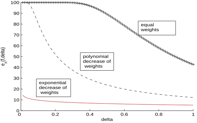
i=1λihi(x),∑iλi=1,λi≥0,let us define the dimension function by

en(f,δ) = T− T

∑

k=1

(1₋λk)

8 ln n

δ2

!

0 0.2 0.4 0.6 0.8 1 0

10 20 30 40 50 60 70 80 90 100

delta

e n

(f,delta)

equal weights

exponential decrease of weights

polynomial decrease of weights

Figure 1: Dimension Function; From top to bottom: equal,polynomial, exponential decay; the x-axis isδ, the y-axis is dimension function value.

The name of this function is motivated by the fact that it can be interpreted as a dimension of a subset of the random convex hull conv(

H

)containing a function approximating f “well enough” (Koltchinskii and Panchenko, 2004). In a way, the dimension function measures the sparsity of the weights in the convex combination f . We plot the dimension function (see Fig. 1) in the cases when T =100,n=1000 and the weights {λi}Ti=1 are equal, polynomially decreasing (λi =i−2) and exponentially decreasing (λi=e(−i+1)). One can see in Fig. 1 that when the weights decrease faster, the dimension function values are uniformly smaller with respect toδ_∈(0,1]. (For different sparsity measures of voting classifiers from convex hulls of VC-major classes see (Koltchinskii et al. (2003a); Koltchinskii and Panchenko (2004); Andonova (2004).)

Theorem 3 (Sparsity bound) For any t>0, with probability at least 1₋e−t, for any n i.i.d. random pairs(X1,Y1), . . . ,(Xn,Yn)randomly drawn with respect to the distributionP, for allλ∈

P

(

H

(Zn)) and f(x) =∑T

i=1λihi(x),

P_{(y f(x)≤0)≤ inf}

0<δ≤1

U1/2+ (P_{n(y f(x)≤}2δ_{) +U+}1

n)

1/22₊1

n, (3.8) where

U= 1

n

t+ln4_δ+en(f,δ)ln G∗(2n,

H

) +en(f,δ)ln( 8

δ2ln n) +ln(8n+4)

.

showing the behavior of the above bound in the case of convex combinations of decision stumps, such as those produced by various boosting algorithms (see Andonova, 2004). There, it is shown experimentally that the sparsity bound is indicative of the generalization performance of a classifier from the convex hull of stumps. For further results and new algorithms, utilizing various notions of sparsity of the weight of convex combinations (see Koltchinskii et al., 2003a). In the case of hard margin SVM classifiers f(x) =∑T

i=1λiK(Xi,x) with uniformly bounded kernels, the bound with marginδbecomes of order

P_{(y f(x)≤0)}min(T,8δ −2_{ln n)}

n ln

n δ, because

en(f,δ)≤min(T,8δ−2ln n).

The inequality for en(f,δ)follows from the inequality(1−λ)p≥1−pλforλ∈[0,1]and p≥1, and the fact that∑T_k=1λk≤1.

This zero-error bound is comparable to the compression bound (Littlestone and Warmuth, 1986) of order _n−T_Tln_Tn,and the bounds of Bartlett and Shawe-Taylor (1999), where U_{∼ n}R_δ22ln2n and

R_≤1 in case of K(x,y)_≤1.When T n the bound in (3.8) is an improvement of the last bound. For example, Tn when SVMs produce very “sparse” solutions (small number of support vectors), that is, the vector of weights(λ1, . . . ,λT)is sparse. The sparseness (in the sense of there being a small number of support vectors) of the solutions of SVMs was recently explored by Steinwart (2003), where lower bounds (of order O(n)) on the number T of support vectors for specific types of kernels were shown; in those cases, the bound in (3.8), relaxed to the upper bound of en(f,δ)≤ min(T,8δ−2_{ln n), is probably not a significant improvement of the result of Bartlett and} Shawe-Taylor (1999). The sparsity of weights of the solutions of SVMs, understood as rapidity of decrease of weights, is in need of further exploration, as it would provide better insight into the bound (3.8) of the generalizations error.

We now notice also that, because en(f,δ)≤min(T,8δ−2ln n)and G∗(n,

H

)≤2n for Problem 1 and G∗(n,

H

)_≤2nd for Problems 2, 3 and G∗(n,

H

) = ne

V

V

,the bound (3.8) is extension of the results of Breiman (1999) for zero-error case, and is similar in nature to the result of Koltchinskii and Panchenko (2004) and Koltchinskii et al. (2003b), but now holding for random classes of functions. Motivations for considering different bounds on the generalization error of classifiers that take into account measures of closeness of random functions in convex combinations and their clustering properties were given by Koltchinskii and Panchenko (2004). We now review those complexities and show bounds on the generalization error, that are similar to the ones proven by Koltchinskii and Panchenko (2004), but applied for different classes of functions. The proofs of the results are similar to those exhibited by Koltchinskii and Panchenko (2004).

Recall that a pointwise variance of h with respect to the distributionλ_∈

P

(

H

(Zn))is defined by

σ2

λ(x) =

Z h(x)₋

Z

h(x)λ(dh)2λ(dh), (3.9) where,σ2_λ(x) =0 if and only if h1(x) =h2(x)for all h1,h2∈

H

(Zn)(Koltchinskii and Panchenko, 2004). The following theorem holds:

Theorem 4 For any t>0 with probability at least 1₋e−t, for any n i.i.d. random pairs(X1,Y1), . . . ,(Xn,Yn) randomly drawn with respect to the distributionP_{, for all}λ_∈

_P

₍

_H

_(Zn_{))and f(x) =}R

P_{(y f(x)≤0) ≤ inf}

0<δ≤γ≤1

2P_{n(y f(x)≤}2δ_{) +4}P_n(σ2_λ(x)≥ γ

3) +

+ 8

n

_56γ

δ2 (ln n)ln G∗(2n,

H

) +ln(8n+4) +t+ln 2γ

δ

+6

n

. (3.10)

The proof is given in Section 4. This time, the proof incorporates random approximations of the classifier function and its variance, Bernstein’s inequality as in (Koltchinskii and Panchenko, 2004), exploring the capacity of random class of the level sets of the margins of the approximating functions and Inequality (3.4).

This result is an improvement of the above margin-bound in the case that the total pointwise variance is small, that is, the classifier functions hi in the convex combination f are close to each other. The constants in the bound are explicit. From the Remark of Theorem 3 in (Koltchinskii and Panchenko, 2004) and the above inequality (3.10), one can see that the quantityP_nσ2

λmight provide

a complexity penalty in the general class of problems defined above.

A result that improves inequality (3.10) by exploring the clustering properties of the convex combination from a random convex hull will now be shown.

Givenλ_∈

P

(

H

(Zn))and f(x) =R

h(x)λ(dh),represent f as

f =

p

∑

j=1 αj

T

∑

k=1 λ(j)

k h

(j)

k

with∑j≤pαj=1,T ≤∞,h(_kj)∈

H

(Zn).

Consider an element c_∈

C

p₍λ_{),that is, c= (}α1_{, . . . ,}α

p,λ1, . . . ,λp), such that αi ∈∆(m) =

n

tkm−k,k∈N,tk ∈ {1,2,3, . . . ,mk}

o

,m_∈N_,λ₌∑p

i=1αiλi,andλi∈

P

(

H

(Zn)),i=1, . . . ,p. De-note by α∗_c =min_{i∈{1,...,p}}αi, where {αi}ip=1 are called the cluster weights. c is interpreted as a decomposition of λ into p clusters as in (Koltchinskii and Panchenko, 2004). For an element c_∈

C

p_{(λ),a weighted variance over clusters is defined by}

σ2_{(c; x) =} p

∑

k=1 α2

kσ2λk(x), (3.11)

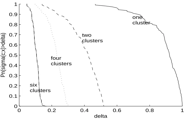
where σ2_λk(x) are defined in (3.9). One can see in Fig. 2 that when the number of the clusters increases, the weighted variance over clusters uniformly decreases (shifts to the left). If there are p small clusters among functions h1, . . . ,hT,then one should be able to choose element c∈

C

p(λ) so thatσ2(c; x)will be small on the majority of data points X1, . . . ,Xn(Koltchinskii and Panchenko, 2004). The following theorem holds:

Theorem 5 For any m_∈N_{, for any t>0 with probability at least 1−e}−t_{, the following is true for}

any n i.i.d. random pairs(X1,Y1), . . . ,(Xn,Yn)randomly drawn with respect to the distributionP, for any p_≥1, c_∈

C

p₍λ_),λ_=∑p

i=1αiλi∈

P

(

H

(Zn)),such thatα1, . . . ,αp∈∆(m)with∑iαi≤1 and f(x) =R

0 0.2 0.4 0.6 0.8 1 0

0.1 0.2 0.3 0.4 0.5 0.6 0.7 0.8 0.9 1

Pn(sigma(c;x)>delta)

delta

one cluster

two clusters

four clusters

six clusters

Figure 2: Empirical distribution of weighted variance over clusters; From right to left: one, tow, four, six clusters; the x-axis isδ.

P_{(y f(x)≤0) ≤ inf}

0<δ≤γ≤1

2P_{n(y f(x)≤}2δ_{) +4}P_n(σ2_{(c; x)≥}γ_{/3) +}

+ 8

n

56pγ

δ2(ln n)ln G∗(2n,

H

) +ln(8n+4) +2 p

∑

j=1 ln

log_mαj α∗

c

+1

+

+ 2 ln

log_m 1 α∗

c

+1

+2p ln 2+t+lnp 2_π4_γ 18δ

+6

n

. (3.12)

The proof is given in the following Section 4. Here, the proof incorporates more sophisticated random approximations of the classifier function and its weighted variance over clusters, Bernstein’s inequality as in (Koltchinskii and Panchenko, 2004), exploring the capacity of random class of the level sets of the margins of the approximating functions and Inequality (3.4). The above bound can be simplified in the following way:

P_{(y f(x)≤0) ≤ inf}

0<δ≤γ≤1

2P_{n(y f(x)≤}2δ_{) +4}P_n(σ2_{(c; x)≥}γ_{/3) +}

+ 8

n

56p γ

δ2(ln n)ln G∗(2n,

H

) +ln(8n+4) +

+ 2(p+1)ln

log_mα1_∗ c

+1

+2p ln 2+t+lnp 2π4γ 18δ

.

Define the number pb_λ(m,n,γ,δ)of(γ,δ)-clusters ofλas the smallest p,for which there exists c_∈

C

_λpsuch that (Koltchinskii and Panchenko, 2004)

P_n(σ2_{(c; x)≥}γ_)≤56p γ

Recall that G∗(n,

H

)_≤2n for Problem 1 and G∗(n,

H

)_≤2nd for Problems 2, 3 and G∗(n,

H

) =

ne V

V

.Then the above simplified bound implies that for all λ=∑_ip₌₁αiλi∈P(

H

(Zn)),such that α1, . . . ,αp∈∆(m)with∑iαi≤1,

P_{(y f(x)≤0)≤K inf}

0<δ≤γ≤1

P_{n(y f(x)≤}δ_{) + pbλ(m,n,}γ_,δ₎ γ

nδ2(ln n)ln G∗(2n,

H

)

+ bp_λ(m,n,γ,δ)

ln

log_mα1∗ c+1

n

.

Observe that ifγ=δ,then

P_{(y f(x)≤0)≤K}P_{n(y f(x)≤}δ_{) + bpλ(m,n,}δ_,δ₎(ln n)ln G∗(2n,

H

)

nδ

+ bp_λ(m,n,δ,δ)

ln

log_mα1∗ c+1

n

.

The above bound is an improvement of the previous bounds in the case when there is a small number pb_λ of clusters so that the resulting weighted variance over clusters is small, and provided that the minimum of the cluster weightsα∗_cis not too small. The bounds shown above are similar in nature to the bounds by Koltchinskii and Panchenko (2004) for base-classes

H

satisfying a general entropy condition. The advantages of the current results are that they are applicable for random classes of functions. The bounds derived here are with explicit constants. For more information regarding the empirical performance of the bounds and the complexities in the case of boosting with stumps and decision trees (see Koltchinskii et al., 2003b; Andonova, 2004). There, it is shown experimentally that generalization bounds based on weighted variance over clusters and margin capture the generalization performance of classifiers produced by several boosting algorithms over decision stumps. Our goal here is to show theoretically the impact of the complexity terms on the generalization performance of functions from random convex hulls, which happen to capture well known algorithms such as SVMs. More experimental evidences are needed to explore the above complexities in the setting of the general problem defined here.

4. Proofs

First we will prove the following lemma that will be used in the proof of Theorem 1.

Lemma 6 For n large enough, if X is a random variable with values in_{0,1_},P(X=1) =p, p_∈

₂

n,1

and X1, . . . ,Xnare independent random realizations of X (Bernoulli trials), then

P 1 n

n

∑

i=1 Xi≥p

!

≥1₄.

Sketch of the Proof of Lemma 6. We want to prove that

P 1 n

n

∑

i=1 Xi≥p

!

=

∑

k≥np

n k

Observe that if n−_n1 <p≤1, then n≥np>n−1 and the inequality becomes pn> n−1 n

n ≥ 1

4, which is true for n_≥2.

Assume that p_≤ n−_n1.The proof of the inequality in this case relies on Poisson and Gaussian approximation to binomial distribution. Let Sn=∑ni=1Xiand Zn= ∑

n i=1(Xi−p)

√

np(1₋p).Notice that

P 1 n

n

∑

i=1 Xi≥p

!

=P(Sn≥np) =P(Zn≥0).

We want to show that there is n0,such that for any n≥n0the following is true for any p∈

₂

n,1− 1 n

P 1 n

n

∑

i=1 Xi≥p

!

≥1₄

From the Poisson-Verteilung approximation theorem, (see Borowkow, 1976, Theorem 7, chapter 5, page 85) it follows that

P(Sn≥µ)≥

∑

k≥np

µk k!e

−µ −µ

2 n,

where µ=np_≥2.From the properties of the Poisson cumulative distribution function F(x_|µ) =

e−µ∑b_i=xc₀µ_i!i,one can see that 1₋F(x_|µ)>1₋F(2_|2)>0.32 for x<µ and µ_≥2.Therefore,

P(Sn≥µ)≥1−F(x|µ)− µ2

n >0.32− µ2

n =0.32−np 2_.

Now, from the Berry-Ess´een Theorem (see Feller, 1966, chapter XVI, page 515) one can derive that

|P(Zn≥0)−0.5|< 33

4 ·

E(X₋EX)3

p

n(E(X₋EX)2₎3 = 33

4 ·

p2_{+ (1−p)}2

p

np(1₋p).

Therefore, P(Zn≥0)>0.5−33₄ ·p

2₊₍₁

−p)2

√

np(1−p).The goal is to find n0 such that for any n≥n0 and

p_∈2_n,1₋1_nthe following is true:

max

n

0.32₋np2,0.5₋33 4 ·

p2+ (1₋p)2

p

np(1₋p)

o

≥1₄.

Let x=np2.One can see that the first term 0.32₋np2=0.32₋x is decreasing with respect to x and the second term 0.5₋33_{4 ·}√p2+(1−p)2

np(1₋p)=0.5−

33 4 ·

p2_+(1−p)2

√

(1−p)(nx)14

is increasing with respect to x.The solution x(n)of the equation

0.32−x=0.5−33 4 ·

x/n+ (1₋x/n)2

r

1₋px/n

(nx)14

Remark: A shorter proof could be achieved if one directly shows that for p∈2 n,1

,

P 1 n

n

∑

i=1 Xi≥p

!

=

∑

k≥np

n k

pk(1₋p)n−k_≥ 1

4.

A stronger version of the above inequality for any p and n was used in (Vapnik (1998), page 133); however, a reference to a proof of this inequality appears currently to be unavailable.

Proof of Theorem 1.

The proof of Inequality (3.4) for random collection of sets of Theorem 1 follows the three main steps - Symmetrization, Randomization and Tail Inequality (see Vapnik (1998); Anthony and Shawe-Taylor (1993)). The difference with other approaches is that the symmetrization step of the proof is carried out for random classes invariant under permutation, after one combines the training set with a ghost sample and uses the incremental property of the random class. Note that sym-metrization for a random subset under similar incremental and permutation properties was proved for the “standard” Vapnik’s inequality by Gat (1999) (bounding the absolute deviation).

Let t>0 be fixed. Assume that n≥2/t2,otherwise if n<2/t2,then 4 exp−nt2/4>1; nothing more need be proved.

Denote the set A=

(

x= (x1, . . . ,xn)∈

Z

n: sup C∈C(x)

P_(C)−1

n∑I(xi∈C)

p

P_(C) ≥t )

.

Assume there exist a set Cx,such that

P_(Cx)−1

n∑I(xi∈Cx)

p

P_(Cx) ≥t. (4.13)

ThenP_(Cx)≥t2_{.We have assumed that t}2_≥ 2

n,thereforeP(Cx)≥ 2 n.

Let x0= (x0₁, . . . ,x0_n) be independent copy of x= (x1, . . . ,xn). It can be observed (see Lemma 6 and Anthony and Shawe-Taylor (1993), Theorem 2.1) that sinceP_{(Cx) =}E_{(I(y∈Cx))≥}2

n, then with probability at least 1/4

P_(Cx)≤ 1

n

∑

I(x

0

i∈Cx). (4.14) From the assumption (4.13) and (4.14), then since √x−a

x+a is a monotone and increasing function in x>0 (a>0), we have that

0<t _≤P(Cx)− 1

n∑I(xi∈Cx)

p P_(Cx)

≤ P(Cx)− 1

n∑I(xi∈Cx)

q

1

2(P(Cx) + 1

n∑I(xi∈Cx))

≤ 1

n∑I(x0i∈Cx)−1_n∑I(xi∈Cx)

q

1 2(

1

n∑I(x0i∈Cx) +1_n∑I(xi∈Cx))

From (4.14) and the above inequality, 1

4I(x∈A) ≤Px0

P_(Cx)≤1

n

∑

I(x

0

i∈Cx)

I(x_∈A)

≤P_x0





1

n∑I(x0i∈Cx)−1_n∑I(xi∈Cx)

q

1 2(

1

n∑I(x0i∈Cx) +1_n∑I(xi∈Cx)) ≥t





≤P_x0



 sup

C∈C(x)

1

n∑I(x0i∈C)−1n∑I(xi∈C)

q

1 2(

1

n∑I(x0i∈C) +1n∑I(xi∈C)) ≥t



.

Taking the expectationE_{x of both sides,}

P_{x sup}

C∈C(x)

P_(C)−1

n∑iI(xi∈C)

p

P_(C) ≥t !

≤

≤4P_x,x0



 sup

C∈C(x)

1

n∑iI(x0i∈C)−1n∑iI(xi∈C)

q

1 2(

1

n∑iI(x0i∈C) +1n∑iI(xi∈C)) ≥t





(using increasing property)

≤4P_x,x0



 sup

C_∈C(x,x0₎

1

n∑iI(x0i∈C)−1n∑iI(xi∈C)

q

1 2(

1

n∑iI(x0i∈C) +1n∑iI(xi∈C)) ≥t

 

(using permutation property)

=4P_x,x0_,ε



 sup

C∈C(x,x0₎

1

n∑iεi(I(x0i∈C)−∑iI(xi∈C))

q

1 2(

1

n∑iI(x0i∈C) +1n∑iI(xi∈C)) ≥t

 

(using Hoeffding-Azuma’s inequality)

≤4E 

∆C(x,x0₎(x1, . . . ,xn,x01, . . . ,x0n)exp˙



₋ nt2

4∑i(Ii−Ii0)2

∑i(Ii+Ii0)



 



≤4E_x,x0

∆C(x,x0₎(x1, . . . ,xn,x01, . . . ,x0n)exp˙

−nt 2 4 =

=4G(2n)exp

−nt 2 4 .

Here the increasing (2.2) and permutation (2.3) properties of the random collection of sets have been used .

Lemma 7 Let Z1, . . . ,Znbe n i.i.d. random variables randomly drawn with respect to the distribu-tionP_{, Zi= (Xi,Yi)∈}

_X

_×

_Y

_{. Let}

C

N,k(Zn) ={C : C={(x,y)∈

X

×

Y

: yg(x)≤δ},g∈

G

N,k(Zn),δ∈[0,1]}, where

G

N,k(Zn) =

(

g : g(z) = 1

N N

∑

i=1

kihi(z),hi∈

H

(Zn),1≤ki≤N−k+1,ki∈N

)

,N,k_∈N

and

H

(Zn)is a random-base class from the general problem. Then

G(n) =E_n∆_C

N,k(Zn)(Z

n_{)≤min(n+1)(N−k+1)}k_(G∗_(n,

_H

₎₎k_,2n_.

If k=N, then ki=1 and

G

N,N(Zn) =

g : g(z) = 1 N∑

N

i=1hi(z),hi∈

H

(Zn) ,where N∈N. In this case, it is clear that G(n) =E_n∆_C

N,N(Zn)(Z

n_{)≤min (n+1)(G∗(n,}

_H

₎₎N_,2n_. Proof.

Following the notation we have to prove that if

H

(Zn)is with finite cardinality H(Zn), then G(n) =E_n∆_C

N,k(Zn)(Z

n_{)≤min(n+1)(N−k+1)}k_E n

H(Zn)k_,2n and if

H

(Zn)is a collection of indicators from the general problem, then

G(n) =E_n∆_C

N,k(Zn)(Z

n₎ ≤min

(n+1)(N₋k+1)kne

V

V k

,2n

.

First, let

H

(Zn)be with finite cardinality H(Zn). Then

card

G

N,k(Zn)≤(N−k+1)kH(Zn)k,

because for each g∈

G

N,k(Zn)there are k different functions hi∈

H

(Zn)participating in the convex combination and the integer coefficients ki∈ {1, . . . ,N−k+1}.Also, for fixed g∈

G

N,k(Zn),it follows that

card

n

{yg(x)_≤δ_}\_{z1, . . . ,zn},δ∈[−1,1]

o

≤(n+1).

(This is clear after re-ordering Y1g(X1), . . . ,Yng(Xn)→Yi1g(Xi1)≤. . .≤Ying(Xin) and taking for values ofδ_{∈ {}Yi1g(Xi1), . . . ,Ying(Xin),1}.) Therefore,

G(n) =E_n∆_C

N,k(Zn)(Z

n₎ ≤min

(n+1)(N₋k+1)kE_nH(Zn₎k_,2n

≤

≤min

(n+1)(N₋k+1)k(G∗(n,

H

))k,2n

.

{C : C={(x,y)_∈

X

_×

Y

: yg(x)_≤δ},g_∈

G

N,k(Zn)}is bounded by(N−k+1)k ne_V

V k

. Similarly to the previous case, for fixed g_∈

G

N,k(Zn),

card

n

{yg(x)_≤δ_}\_{z1, . . . ,zn},δ∈[0,1]

o

≤(n+1),

and therefore

G(n) =E_n∆_C

N,k(Zn)(Z

n₎ ≤min

(n+1)(N₋k+1)kne

V

V k

,2n

=

=min(n+1)(N₋k+1)k_(G∗_(n,

_H

₎₎k_,2n_.

Next, the proofs of Theorem 2,3, 4 and 5 are shown. They follow closely the proofs given by Koltchinskii and Panchenko (2004) and Koltchinskii et al. (2003b) for non random classes of func-tions. We adjust the proofs to hold for random classes of functions by using Inequality 3.4 from Theorem 1.

Define the function

φ(a,b) = (a−b)

2

a I(a≥b),

that is convex for a>0 and increasing with respect to a,decreasing with respect to b. Proof of Theorem 2.

Let Z1= (X1,Y1), . . . ,Zn= (Xn,Yn)be i.i.d samples randomly drawn with respect to the distri-butionP_{.Let us first fix}δ_{∈(0,1]and let f =}∑_kT₌₁λ_{khk ∈conv(}

_H

_(Zn_{))be any function from the}

convex hull of

H

(Zn),where

H

(Zn)is the random-base class defined in the general problem. Given N _≥1, generate i.i.d sequence of functions ξ1, . . . ,ξN according to the distribution λ=

(λ1, . . . ,λT),Pξ(ξi=hk) =λkfor k=1, . . . ,T andξiare independent of{(Xk,Yk)}_kn₌₁.ThenEξξi(x) = ∑T

k=1λkhk(x).

Consider a function

g(x) = 1

N N

∑

k=1 ξk(x),

which plays the role of a random approximation of f in the following sense:

P_{(y f(x)≤0) =}P

y f(x)_≤0,yg(x)_≤δ+P

y f(x)_≤0,yg(x)>δ

≤P

yg(x)_≤δ+E_x,yP_ξ

E_{ξyg(x)≤0,yg(x)≥}δ

≤P

yg(x)_≤δ+E_x,yP_ξ

yg(x)₋E_ξyg(x)≥δ

=P

yg(x)_≤δ+E_x,yP_ξ

N

∑

k=1

(yξi(x)−yEξξi(x))≥Nδ

!

≤P_yg(x)≤δ_+exp−Nδ

2 2

, (4.15)

where in the last step is applied Hoeffding- ˇCernoff inequality. Then,

P

y f(x)_≤0

≤P

Similarly to the above inequality, one can derive that,

E_ξP_n

yg(x)_≤δ_≤P_n

y f(x)_≤2δ+exp(₋Nδ2/2). (4.17) For any random realization of the sequenceξ1, . . . ,ξN,the random function g belongs to the class

G

N(Zn) =

n

1 N∑

N

i=1hi(x): hi∈

H

(Zn)

o

.

Consider the random collection of level sets for fixed N_∈N_,

C

(Zn) =nC=_{(x,y)_∈

X

×

Y

: yg(x)_≤δ_},g_∈

G

N(Zn),δ∈(0,1]

o

.

Clearly

C

(Zn)satisfies conditions (2.2) and (2.3). In order to apply the inequality for the random collection of sets (3.4), one has to estimate G(n) =En∆_C(Zn₎(Zn). By Lemma 7 it follows that G(n)_≤(G∗(n,

H

))N_(n+1).

From this and Theorem 1, we have

Pn _sup

C∈C(Zn₎

P_(C)−1

n∑ n

i=1I(Xi∈C)

p

P_(C) ≥t

!

≤ 4G(2n)e−nt24 ≤

≤ 4(G∗(2n,

H

))N(2n+1)e−nt24 =_e−u,

where a change of variables t =q4

n(u+N ln(G∗(2n,

H

)) +ln(8n+4)) is made. So, for a fixed δ∈(0,1],for any u>0 with probability at least 1−e−u, it follows that

P(yg(x)_≤δ)₋1 n∑

n

i=1I(Yig(Xi)≤δ)

p

P_(yg(x)≤δ₎ ≤ r

4

n(u+N ln(G∗(2n,

H

)) +ln(8n+4)). (4.18) The functionφ(a,b),a>0 is convex. Therefore,

E_ξφ

P_(yg(x)≤δ_),P_n(yg(x)≤δ₎

≥φE_ξP_(yg(x)≤δ_),E_ξP_n(yg(x)≤δ₎

.

Based on the monotonic properties ofφ(a,b)and inequalities (4.16) and (4.17), it is obtained that for anyδ_∈(0,1],for any u>0 with probability at least 1₋e−u_,

φP_{(y f(x)≤0)−exp(−}Nδ2_/2),P_{n(y f(x)≤}2δ_+exp(−Nδ2_/2))

≤

≤4_n(u+N ln(G∗(2n,

H

)) +ln(8n+4)). (4.19) Choose N=2 ln n_δ2 ,such that exp(−Nδ2/2) =

1 n.Take U=1

n

u+2 ln n

δ2 ln(G∗(2n,

H

)) +ln(8n+4)

.

Solving the above inequality with respect toP_{(y f(x)≤0),it follows that}

P_{(y f(x)≤0)≤} √_U+ r

P_{n(y f(x)≤}2δ_{) +}1

n+U

!2

+1

In order to make the bound uniform with respect toδ∈(0,1],we apply standard union bound techniques (Koltchinskii and Panchenko, 2004). First, we prove the uniformity forδ_∈∆=_{2−k,k=

0,1, . . . .._}. Apply the above inequality for fixedδ_∈∆by replacing u by u+ln2_δ and hence e−u replaced by δ₂e−u.Denote

U0=1

n

u+ln2 δ+

2 ln n

δ2 ln(G∗(2n,

H

)) +ln(8n+4)

.

Then

P



\

δ∈∆

n

P_{(y f(x)≤0)≤} √_U0₊

r

P_{n(y f(x)≤}2δ_{) +}1

n+U0

!2

+1

n

o

_≥

≥1₋e−u

∞

∑

k=1

2−k_≥1₋e−u.

Now, in order to make the bound for any δ_∈(0,1],observe that if δ0 _∈(0,1] then there is k_∈

Z_+,2−k−1_≤δ0_<2−k_.

Therefore, if the above bound holds for fixedδ0_∈(0,1],then

P_{n(y f(x)≤}δ0_)≤P_n

y f(x)_≤2−k

and

1/δ2

0≤22k+2,ln 2

δ0 ≤ln 2k+2. So, changing the constants in the bound, denote

U=1

n

t+ln4 δ+

8 ln n

δ2 ln(G∗(2n,

H

)) +ln(8n+4)

.

It follows that, for any t>0 with probability at least 1₋e−tfor anyδ_∈(0,1],the following holds:

P_{(y f(x)≤0)≤} √_U+ r

P_{n(y f(x)≤}2δ_{) +}1

n+U

!2

+1

n

Thus, the Theorem 2 and inequality (3.6) hold.

Now, the proof of Sparsity bound of Theorem 3 will be shown. Denote∆=_{2−k: k≥1}and z= (x,y),Zn=(X1,Y1), . . . ,(Xn,Yn)

.

Let us fix f(x) =∑T_k=1λkhk(x)∈ conv(

H

(Zn)).Given N≥1, generate an i.i.d. sequence of func-tionsξ1, . . . ,ξNaccording to the distributionPξ(ξi(x) =hk(x)) =λkfor k=1, . . . ,T and independent of_{(Xi,Yi)}ni=1.Clearly,Eξξi(x) =∑Tk=1λkhk(x).Consider the function

g(x) = 1

N N

∑