Lossless Online Bayesian Bagging
Herbert K. H. Lee [email protected]
Department of Applied Math and Statistics School of Engineering
University of California, Santa Cruz Santa Cruz, CA 95064, USA
Merlise A. Clyde [email protected]
Institute of Statistics and Decision Sciences Box 90251
Duke University
Durham, NC 27708, USA
Editor:Bin Yu
Abstract
Bagging frequently improves the predictive performance of a model. An online version has recently been introduced, which attempts to gain the benefits of an online algorithm while approximating regular bagging. However, regular online bagging is an approximation to its batch counterpart and so is not lossless with respect to the bagging operation. By operating under the Bayesian paradigm, we introduce an online Bayesian version of bagging which is exactly equivalent to the batch Bayesian version, and thus when combined with a lossless learning algorithm gives a completely lossless online bagging algorithm. We also note that the Bayesian formulation resolves a theoretical problem with bagging, produces less variability in its estimates, and can improve predictive performance for smaller data sets.
Keywords: Classification Tree, Bayesian Bootstrap, Dirichlet Distribution
1. Introduction
In a typical prediction problem, there is a trade-off between bias and variance, in that after a certain amount of fitting, any increase in the precision of the fit will cause an increase in the prediction variance on future observations. Similarly, any reduction in the prediction variance causes an increase in the expected bias for future predictions. Breiman (1996) introduced bagging as a method of reducing the prediction variance without affecting the prediction bias. As a result, predictive performance can be significantly improved.
procedures. Breiman (1994) demonstrated that tree models, among others, are empirically unstable.
Online bagging (Oza and Russell, 2001) was developed to implement bagging sequen-tially, as the observations appear, rather than in batch once all of the observations have arrived. It uses an asymptotic approximation to mimic the results of regular batch bagging, and as such it is not a lossless algorithm. Online algorithms have many uses in modern computing. By updating sequentially, the update for a new observation is relatively quick compared to re-fitting the entire database, making real-time calculations more feasible. Such algorithms are also advantageous for extremely large data sets where reading through the data just once is time-consuming, so batch algorithms which would require multiple passes through the data would be infeasible.
In this paper, we consider a Bayesian version of bagging (Clyde and Lee, 2001) based on the Bayesian bootstrap (Rubin, 1981). This overcomes a technical difficulty with the usual bootstrap in bagging. It also leads to a theoretical reduction in variance over the bootstrap for certain classes of estimators, and a significant reduction in observed variance and error rates for smaller data sets. We present an online version which, when combined with a lossless online model-fitting algorithm, continues to be lossless with respect to the bagging operation, in contrast to ordinary online bagging. The Bayesian approach requires the learning base algorithm to accept weighted samples.
In the next section we review the basics of the bagging algorithm, of online bagging, and of Bayesian bagging. Next we introduce our online Bayesian bagging algorithm. We then demonstrate its efficacy with classification trees on a variety of examples.
2. Bagging
In ordinary (batch) bagging, bootstrap re-sampling is used to reduce the variability of an unstable estimator. A particular model or algorithm, such as a classification tree, is specified for learning from a set of data and producing predictions. For a particular data set Xm,
denote the vector of predictions (at the observed sites or at new locations) by G(Xm). Denote the observed data by X = (x1, . . . , xn). A bootstrap sample of the data is a
sample with replacement, so that Xm = (xm1, . . . , xmn), where mi ∈ {1, . . . , n} with
repetitions allowed. Xm can also be thought of as a re-weighted version of X, where the
weights,ωi(m)are drawn from the set{0,n1,2n, . . . ,1}, i.e.,nωi(m)is the number of times that xiappears in themth bootstrap sample. We denote the weighted sample as(X, ω(m)). For each bootstrap sample, the model produces predictions G(Xm) =G(Xm)1, . . . , G(Xm)P
whereP is the number of prediction sites. M total bootstrap samples are used. The bagged predictor for thejth element is then
1 M
M X
m=1
G(Xm)j =
1 M
M X
m=1
G(X,ω(m))j,
or in the case of classification, thejth element is predicted to belong to the most frequently predicted category byG(X1)j, . . . , G(XM)j.
A version of pseudocode for implementing bagging is
(a) Draw a bootstrap sample,Xm, fromX.
(b) Find predicted valuesG(Xm).
2. The bagging predictor is M1 PMm=1G(Xm).
Equivalently, the bootstrap sample can be converted to a weighted sample(X, ω(m))where
the weightsωi(m)are found by taking the number of timesxiappears in the bootstrap sample and dividing by n. Thus the weights will be drawn from {0,n1,2n, . . . ,1} and will sum to 1. The bagging predictor using the weighted formulation is M1 PMm=1G(Xm, ω(m)) for regression, or the plurality vote for classification.
2.1 Online Bagging
Online bagging (Oza and Russell, 2001) was recently introduced as a sequential approxima-tion to batch bagging. In batch bagging, the entire data set is collected, and then bootstrap samples are taken from the whole database. An online algorithm must process observations as they arrive, and thus each observation must be resampled a random number of times when it arrives. The algorithm proposed by Oza and Russell resamples each observation according to a Poisson random variable with mean 1, i.e.,P(Km =k) = exp(−1)/k!, where
Km is the number of resamples in “bootstrap sample” m, Km ∈ {0,1, . . .}. Thus as each
observation arrives, it is addedKm times toXm, and then G(Xm) is updated, and this is
done form∈ {1, . . . , M}.
Pseudocode for online bagging is
Fori∈ {1, . . . , n},
1. Form∈ {1, . . . , M},
(a) Draw a weight Km from a Poisson(1) random variable and add Km copies
ofxi toXm.
(b) Find predicted valuesG(Xm).
2. The current bagging predictor is M1 PMm=1G(Xm).
Ideally, step 1(b) is accomplished with a lossless online update that incorporates the Km
new points without refitting the entire model. We note thatnmay not be known ahead of time, but the bagging predictor is a valid approximation at each step.
Online bagging is not guaranteed to produce the same results as batch bagging. In particular, it is easy to see that after n points have been observed, there is no guarantee that Xm will contain exactly n points, as the Poisson weights are not constrained to add
2.2 Bayesian Bagging
Ordinary bagging is based on the ordinary bootstrap, which can be thought of as replacing the original weights of n1 on each point with weights from the set{0,n1,2n, . . . ,1}, with the total of all weights summing to 1. A variation is to replace the ordinary bootstrap with the Bayesian bootstrap (Rubin, 1981). The Bayesian approach treats the vector of weights ω as unknown parameters and derives a posterior distribution forω, and henceG(X, ω). The non-informative priorQni=1ωi−1, when combined with the multinomial likelihood, leads to a Dirichletn(1, . . . ,1) distribution for the posterior distribution of ω. The full posterior
distribution of G(X, ω) can be estimated by Monte Carlo methods: generate ω(m) from
a Dirichletn(1, . . . ,1) distribution and then calculate G(X, ω(m)) for each sample. The
average of G(X, ω(m)) over the M samples corresponds to the Monte Carlo estimate of
the posterior mean of G(X, ω) and can be viewed as a Bayesian analog of bagging (Clyde and Lee, 2001).
In practice, we may only be interested in a point estimate, rather than the full posterior distribution. In this case, the Bayesian bootstrap can be seen as a continuous version of the regular bootstrap. Thus Bayesian bagging can be achieved by generating M Bayesian bootstrap samples, and taking the average or majority vote of the G(X, ω(m)). This is
identical to regular bagging except that the weights are continuous-valued on (0,1), instead of being restricted to the discrete set{0,1n,n2, . . . ,1}. In both cases, the weights must sum to 1. In both cases, the expected value of a particular weight is n1 for all weights, and the expected correlation between weights is the same (Rubin, 1981). Thus Bayesian bagging will generally have the same expected point estimates as ordinary bagging. The variability of the estimate is slightly smaller under Bayesian bagging, as the variability of the weights is nn+1 times that of ordinary bagging. As the sample size grows large, this factor becomes arbitrarily close to one, but we do note that it is strictly less than one, so the Bayesian approach does give a further reduction in variance compared to the standard approach. In practice, for smaller data sets, we often find a significant reduction in variance, possibly because the use of continuous-valued weights leads to fewer extreme cases than discrete-valued weights.
Pseudocode for Bayesian bagging is
1. Form∈ {1, . . . , M},
(a) Draw random weightsω(m) from aDirichletn(1, . . . ,1) to produce the Bayesian
bootstrap sample(X, ω(m)).
(b) Find predicted valuesG(X, ω(m)).
2. The bagging predictor is M1 PMm=1 G(X, ω(m)).
Use of the Bayesian bootstrap does have a major theoretical advantage, in that for some problems, bagging with the regular bootstrap is actually estimating an undefined quantity. To take a simple example, suppose one is bagging the fitted predictions for a point y from a least-squares regression problem. Technically, the full bagging estimate is
1
M0
P
myˆm where m ranges over all possible bootstrap samples, M0 is the total number of possible bootstrap samples, and ˆym is the predicted value from the model fit using the
first data point replicated n times, and no other data points. For this bootstrap sample, the regression model is undefined (since at least two different points are required), and so ˆ
y and thus the bagging estimator are undefined. In practice, only a small sample of the possible bootstrap samples is used, so the probability of drawing a bootstrap sample with an undefined prediction is very small. Yet it is disturbing that in some problems, the bagging estimator is technically not well-defined. In contrast, the use of the Bayesian bootstrap completely avoids this problem. Since the weights are continuous-valued, the probability that any weight is exactly equal to zero is zero. Thus with probability one, all weights are strictly positive, and the Bayesian bagging estimator will be well-defined (assuming the ordinary estimator on the original data is well-defined).
We note that the Bayesian approach will only work with models that have learning al-gorithms that handle weighted samples. Most standard models either have readily available such algorithms, or their algorithms are easily modified to accept weights, so this restriction is not much of an issue in practice.
3. Online Bayesian Bagging
Regular online bagging cannot be exactly equivalent to the batch version because the Poisson counts cannot be guaranteed to sum to the number of actual observations. Gamma random variables can be thought of as continuous analogs of Poisson counts, which motivates our derivation of Bayesian online bagging. The key is to recall a fact from basic probability — a set of independent gamma random variables divided by its sum has a Dirichlet distribution, i.e.,
If wi∼Γ(αi,1), then µ
w1
P
wi
,Pw2
wi
, . . . ,Pwk
wi 
∼Dirichletn(α1, α2, . . . , αk).
(See for example, Hogg and Craig, 1995, pp. 187–188.) This relationship is a common method for generating random draws from a Dirichlet distribution, and so is also used in the implementation of batch Bayesian bagging in practice.
Thus in the online version of Bayesian bagging, as each observation arrives, it has a realization of a Gamma(1) random variable associated with it for each bootstrap sample, and the model is updated after each new weighted observation. If the implementation of the model requires weights that sum to one, then within each (Bayesian) bootstrap sample, all weights can be re-normalized with the new sum of gammas before the model is updated. At any point in time, the current predictions are those aggregated across all bootstrap samples, just as with batch bagging. If the model is fit with an ordinary lossless online algorithm, as exists for classification trees (Utgoff et al., 1997), then the entire online Bayesian bagging procedure is completely lossless relative to batch Bayesian bagging. Furthermore, since batch Bayesian bagging gives the same mean results as ordinary batch bagging, online Bayesian bagging also has the same expected results as ordinary batch bagging.
Pseudocode for online Bayesian bagging is
Fori∈ {1, . . . , n},
(a) Draw a weight ω(im) from aGamma(1,1) random variable, associate weight withxi, and add xi toX.
(b) Find predicted valuesG(X, ω(m))(renormalizing weights if necessary).
2. The current bagging predictor is M1 PMm=1G(X, ω(m)).
In step 1(b), the weights may need to be renormalized (by dividing by the sum of all current weights) if the implementation requires weights that sum to one. We note that for many models, such as classification trees, this renormalization is not a major issue; for a tree, each split only depends on the relative weights of the observations at that node, so nodes not involving the new observation will have the same ratio of weights before and after renormalization and the rest of the tree structure will be unaffected; in practice, in most implementations of trees (including that used in this paper), renormalization is not necessary. We discuss the possibility of renormalization in order to be consistent with the original presentation of the bootstrap and Bayesian bootstrap, and we note that ordinary online bagging implicitly deals with this issue equivalently.
The computational requirements of Bayesian versus ordinary online bagging are com-parable. The procedures are quite similar, with the main difference being that the fitting algorithm must handle non-integer weights for the Bayesian version. For models such as trees, there is no significant additional computational burden for using non-integer weights.
4. Examples
We demonstrate the effectiveness of online Bayesian bagging using classification trees. Our implementation uses the lossless online tree learning algorithms (ITI) of Utgoff et al. (1997) (available at http://www.cs.umass.edu/∼lrn/iti/). We compared Bayesian bagging to a single tree, ordinary batch bagging, and ordinary online bagging, all three of which were done using the minimum description length criterion (MDL), as implemented in the ITI code, to determine the optimal size for each tree. To implement Bayesian bagging, the code was modified to account for weighted observations.
We use a generalized MDL to determine the optimal tree size at each stage, replacing all counts of observations with the sum of the weights of the observations at that node or leaf with the same response category. Replacing the total count directly with the sum of the weights is justified by looking at the multinomial likelihood when written as an exponential family in canonical form; the weights enter through the dispersion parameter and it is easily seen that the unweighted counts are replaced by the sums of the weights of the observations that go into each count. To be more specific, a decision tree typically operates with a multinomial likelihood,
Y
leavesj Y
classesk
pnjk
jk ,
wherepjk is the true probability that an observation in leaf j will be in class k, and njk is
the count of data points in leaf j in class k. This is easily re-written as the product over all observations, Qni=1p∗i where if observation i is in leaf j and a member of class k then p∗
i = pjk. For simplicity, we consider the case k = 2 as the generalization to larger k is
where p is the true probability that y = 1. Writing the likelihood in exponential family form gives expn ³yθ+ log1+exp1 {θ}´.aowhereais the dispersion parameter, which would be equal to 1 for a standard data set, but would be the reciprocal of the weight for that observation in a weighted data set. Thus the likelihood for an observation y with weight w is expn ³yθ+ log1+exp1 {θ}´.(1/w)o = pwy(1−p)w(1−y) and so returning to the full multinomial, the original counts are simply replaced by the weighted counts. As MDL is a penalized likelihood criterion, we thus use the weighted likelihood and replace each count with a sum of weights. We note that for ordinary online bagging, using a single Poisson weightK with our generalized MDL is exactly equivalent to includingK copies of the data point in the data set and using regular MDL.
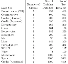
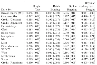
Table 1 shows the data sets we used for classification problems, the number of classes in each data set, and the sizes of their respective training and test partitions. Table 2 displays the results of our comparison study. All of the data sets, except the final one, are avail-able online athttp://www.ics.uci.edu/∼mlearn/MLRepository.html, the UCI Machine Learning Repository. The last data set is described in Lee (2001). We compare the results of training a single classification tree, ordinary batch bagging, online bagging, and Bayesian online bagging (or equivalently Bayesian batch). For each of the bagging techniques, 100 bootstrap samples were used. For each data set, we repeated 1000 times the following pro-cedure: randomly choose a training/test partition; fit a single tree, a batch bagged tree, an online bagged tree, and a Bayesian bagged tree; compute the misclassification error rate for each fit. Table 2 reports the average error rate for each method on each data set, as well as the estimated standard error of this error rate.
Size of Size of Number of Training Test Data Set Classes Data Set Data Set Breast cancer (WI) 2 299 400
Contraceptive 3 800 673
Credit (German) 2 200 800
Credit (Japanese) 2 290 400
Dermatology 6 166 200
Glass 7 164 50
House votes 2 185 250
Ionosphere 2 200 151
Iris 3 90 60
Liver 3 145 200
Pima diabetes 2 200 332
SPECT 2 80 187
Wine 3 78 100
Mushrooms 2 1000 7124
Spam 2 2000 2601
Credit (American) 2 4000 4508
Bayesian Single Batch Online Online/Batch
Data Set Tree Bagging Bagging Bagging
Breast cancer (WI) 0.055 (.020) 0.045 (.010) 0.045 (.010) 0.041 (.009) Contraceptive 0.522 (.019) 0.499 (.017) 0.497 (.017) 0.490 (.016) Credit (German) 0.318 (.022) 0.295 (.017) 0.294 (.017) 0.285 (.015) Credit (Japanese) 0.155 (.017) 0.148 (.014) 0.147 (.014) 0.145 (.014) Dermatology 0.099 (.033) 0.049 (.017) 0.053 (.021) 0.047 (.019) Glass 0.383 (.081) 0.357 (.072) 0.361 (.074) 0.373 (.075) House votes 0.052 (.011) 0.049 (.011) 0.049 (.011) 0.046 (.010) Ionosphere 0.119 (.026) 0.094 (.022) 0.099 (.022) 0.096 (.021) Iris 0.062 (.029) 0.057 (.026) 0.060 (.025) 0.058 (.025) Liver 0.366 (.036) 0.333 (.032) 0.336 (.034) 0.317 (.033) Pima diabetes 0.265 (.027) 0.250 (.020) 0.247 (.021) 0.232 (.017) SPECT 0.205 (.029) 0.200 (.030) 0.202 (.031) 0.190 (.027) Wine 0.134 (.042) 0.094 (.037) 0.101 (.037) 0.085 (.034) Mushrooms 0.004 (.003) 0.003 (.002) 0.003 (.002) 0.003 (.002) Spam 0.099 (.008) 0.075 (.005) 0.077 (.005) 0.077 (.005) Credit (American) 0.350 (.007) 0.306 (.005) 0.306 (.005) 0.305 (.006)
Table 2: Comparison of average classification error rates (with standard error)
We note that in all cases, both online bagging techniques produce results similar to ordinary batch bagging, and all bagging methods significantly improve upon the use of a single tree. However, for smaller data sets (all but the last three), online/batch Bayesian bagging typically both improves prediction performance and decreases prediction variability.
5. Discussion
Bagging is a useful ensemble learning tool, particularly when models sensitive to small changes in the data are used. It is sometimes desirable to be able to use the data in an online fashion. By operating in the Bayesian paradigm, we can introduce an online algorithm that will exactly match its batch Bayesian counterpart. Unlike previous versions of online bagging, the Bayesian approach produces a completely lossless bagging algorithm. It can also lead to increased accuracy and decreased prediction variance for smaller data sets.
Acknowledgments
References
L. Breiman. Heuristics of instability in model selection. Technical report, University of California at Berkeley, 1994.
L. Breiman. Bagging predictors. Machine Learning, 26(2):123–140, 1996.
M. A. Clyde and H. K. H. Lee. Bagging and the Bayesian bootstrap. In T. Richardson and T. Jaakkola, editors, Artificial Intelligence and Statistics 2001, pages 169–174, 2001.
R. V. Hogg and A. T. Craig. Introduction to Mathematical Statistics. Prentice-Hall, Upper Saddle River, NJ, 5th edition, 1995.
H. K. H. Lee. Model selection for neural network classification. Journal of Classification, 18:227–243, 2001.
N. C. Oza and S. Russell. Online bagging and boosting. In T. Richardson and T. Jaakkola, editors, Artificial Intelligence and Statistics 2001, pages 105–112, 2001.
D. B. Rubin. The Bayesian bootstrap. Annals of Statistics, 9:130–134, 1981.