Wavelet decompositions of Random Forests - smoothness
analysis, sparse approximation and applications
Oren Elisha School of Mathematical Sciences University of Tel-Aviv
and GE Global Research Israel
Shai Dekel School of Mathematical Sciences
University of Tel-Aviv
and GE Global Research
Israel
Editors:Lawrence Carin
Abstract
In this paper we introduce, in the setting of machine learning, a generalization of wavelet
analysis which is a popular approach to low dimensional structured signal analysis. The
wavelet decomposition of a Random Forest provides a sparse approximation of any
regres-sion or classification high dimenregres-sional function at various levels of detail, with a concrete ordering of the Random Forest nodes: from ‘significant’ elements to nodes capturing only
‘insignificant’ noise. Motivated by function space theory, we use the wavelet
decomposi-tion to compute numerically a ‘weak-type’ smoothness index that captures the complexity
of the underlying function. As we show through extensive experimentation, this sparse representation facilitates a variety of applications such as improved regression for difficult
datasets, a novel approach to feature importance, resilience to noisy or irrelevant features,
compression of ensembles, etc.
Keywords: Random Forest, Wavelets, Besov spaces, adaptive approximation, feature importance.
1. Introduction
Our work brings together Function Space theory, Harmonic Analysis and Machine
Learn-ing for the analysis of high dimensional big data. In the field of (low-dimensional) signal
processing, there is a complete theory that models structured datasets (e.g audio, images, video) as functions in certain Besov spaces (DeVore 1998), (DeVore et. al. 1992). When
the performance of adaptive approximation and is used in a variety of applications, such as
denoising, compression, feature extraction, etc. using very simple algorithms.
The first contribution of this work is a construction of wavelet decomposition of
Ran-dom Forests (Breiman 2001), (Biau and Scornet 2016), (Denil et. al. 2014). Wavelets
(Daubechies 1992), (Mallat 2009) and geometric wavelets (Dekel and Leviatan 2005), (Alani et. al 2007), (Dekel and Gershtansky 2012), are a powerful yet simple tool for
con-structing sparse representations of ‘complex’ functions. The Random Forest (RF) (Biau
and Scornet 2016), (Criminisi et. al. 2011), (Hastie et. al. 2009) introduced by Breiman (Breiman 2001), (Breiman 1996), is a very effective machine learning method that can be
considered as a way to overcome the ‘greedy’ nature and high variance of a single decision
tree. When combined, the wavelet decomposition of the RF unravels the sparsity of the underlying function and establishes an order of the RF nodes from ‘important’ components
to ‘negligible’ noise. Therefore, the method provides a better understanding of any
con-structed RF. This helps to avoid over-fitting in certain scenarios (e.g. small number of trees), to remove noise or provide compression. Our approach could also be considered
as an alternative method for pruning of ensembles (Chen et. al. 2009), (Kulkarni and
Sinha 2012), (Yang et. al. 2012), (Joly et. al. 2012) where the most important decision nodes of a huge and complex ensemble of models can be quickly and efficiently extracted.
Thus, instead of controlling complexity by restricting trees’ depth or node size, one controls complexity through adaptive wavelet approximation.
Our second contribution is to generalize the function space characterization of adaptive algorithms (DeVore 1998), (Devore and Lorentz 1993), to a typical machine learning setup.
Using the wavelet decomposition of a RF, we can actually numerically compute a ‘weak-type’
smoothness index of the underlying regression or classification function overcoming noise. We prove the first part of the characterization and demonstrate, using several examples,
the correspondence between the smoothness of the underlying function and properties such
as compression.
Applying a ‘wavelet-type’ machinery for learning tasks, using ‘Treelets’, was introduced
by (Lee et. al. 2008). Treelets provide a decomposition of the domain into localized basis functions that enable a sparse representation of smooth signals. This method performs
a bottom-up construction in the feature space, where at each step, a local PCA among
two correlated variables generates a new node in a tree. Our method is different, since for supervised learning tasks, the response variable should be used during the construction of
the adaptive representation. Also, our work significantly improves upon the ‘wavelet-type’
construction of (Gavish et. al. 2010). First, since our wavelet decomposition is built on the solid foundations of RFs, it leverages on the well-known fact that over-complete
in problems such as regression, estimation, etc. Secondly, from the theoretical perspective,
the Lipschitz space analysis of (Gavish et. al. 2010) is generalized by our Besov space
analysis, which is the right mathematical setup for adaptive approximation using wavelets.
The paper is organized as follows: In Section 2 we review Random Forests. In Section
3 we present our main wavelet construction and list some of its key properties. In section
4 we present some theoretical aspects of function space theory and its connection to spar-sity. This characterization quantifies the sparsity of the data with respect to the response
variable. In Section 5 we review how a novel form of Variable Importance (VI) is computed
using our approach. Section 6 provides extensive experimental results that demonstrate the applicative added value of our method in terms of regression, classification, compression
and variable importance quantification.
2. Overview of Random Forests
We begin with an overview of single trees. In statistics and machine learning (Breiman
et. al. 1984), (Alpaydin 2004), (Biau and Scornet 2016), (Denil et. al. 2014), (Hastie et. al. 2009) the construction is called a Decision Tree or the Classification and Regression
Tree (CART) while in image processing and computer graphics (Radha et. al. 1996),
(Salembier and Garrido 2000) it is coined as the Binary Space Partition (BSP) tree. We are given a real-valued function f ∈L2(Ω0) or a discrete dataset{xi∈Ω0, f(xi)}i∈I, in some convex bounded domain Ω0 ⊂ Rn. The goal is to find an efficient representation of the
underlying function, overcoming the complexity, geometry and possibly non-smooth nature of the function values. To this end, we subdivide the initial domain Ω0 into two subdomains, e.g. by intersecting it with a hyper-plane. The subdivision is performed to minimize a given
cost function. This subdivision process then continues recursively on the subdomains until some stopping criterion is met, which in turn, determines the leaves of the tree. We now
describe one instance of the cost function which is related to minimizing variance. At each
stage of the subdivision process, at a certain node of the tree, the algorithm finds, for the convex domain Ω⊂Rn associated with the node:
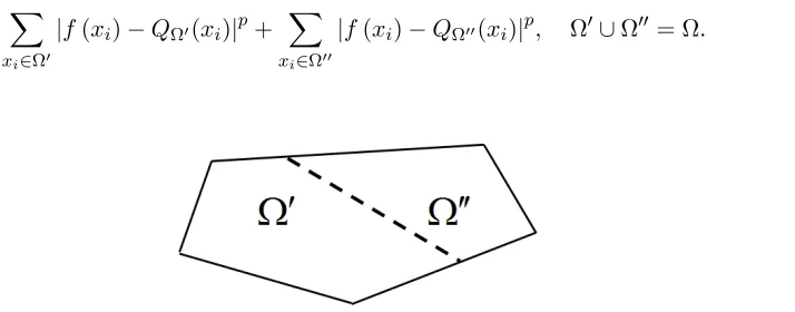
(i) A partition by an hyper-plane into two convex subdomains Ω0,Ω00 (see Figure 1),
(ii) Two multivariate polynomials QΩ0, QΩ00 ∈ Πr−1(Rn), of fixed (typically low) total
degree r −1.
The subdomains and the polynomials are chosen to minimize the following quantity
kf −QΩ0kp
Lp(Ω0)+kf −QΩ
00kp
Lp(Ω00), Ω
Here, for 1≤p <∞, we used the definition
kgkL
p(Ω˜) :=
Z
˜ Ω
|g(x)|pdx
1/p
,
If the dataset is discrete, consisting of feature vectors xi ∈Rn, i∈I , with response values
f(xi), then a discrete functional is minimized
X
xi∈Ω0
|f(xi)−QΩ0(xi)|p+
X
xi∈Ω00
|f(xi)−QΩ00(xi)|p, Ω0∪Ω00 = Ω. (2)
Figure 1: Illustration of a subdivision by an hyperplane of a parent domain Ω into two children Ω0,Ω00.
Observe that for any given subdividing hyperplane, the approximating polynomials in
(2) can be uniquely determined forp= 2 by least square minimization (see (Avery)) for a
survey of local polynomial regression). For the orderr= 1, the approximating polynomials are nothing but the mean of the function values over each of the subdomains
QΩ0(x) =CΩ0 = 1
#{xi∈Ω0} X
xi∈Ω0
f(xi), QΩ00(x) =CΩ00= 1
#{xi ∈Ω00} X
xi∈Ω00
f(xi).
(3) In many applications of decision trees, the high-dimensionality of the data does not allow to
search through all possible subdivisions. As in our experimental results, one may restrict the
subdivisions to the class of hyperplanes aligned with the main axes. In contrast, there are cases where one would like to consider more advanced form of subdivisions, where they take
certain hyper-surface form, such as conic-sections. Our paradigm of wavelet decompositions
can support in principle all of these forms.
Random Forest (RF) is a popular machine learning tool that collects decision trees into
an ensemble model (Breiman 2001), (Bernard et. al 2012), (Biau 2012), (Biau and Scornet
2016). The trees are constructed independently in a diverse fashion and prediction is done by a voting mechanism among all trees. A key element (Breiman 2001), is that large
that differ in the way randomness is injected into the model, e.g bagging, random feature
subset selection and the partition criterion (Boulesteix et. al. 2012), (Criminisi et. al.
2011), (Hastie et. al. 2009). Our wavelet decomposition paradigm is applicable to most of the RF versions known from the literature.
Bagging (Breiman 1996) is a method that produces partial replicates of the training data
for each tree. A typical approach is to randomly select for each tree a certain percentage of
the training set (e.g. 80%) or to randomly select samples with repetitions (Hastie et. al. 2009). From an approximation theoretical perspective, this form of RF allows to create an
over-complete representation (Christensen 2002) of the underlying function that overcomes
the ‘greedy’ nature of a single tree .
Additional methods to inject randomness can be achieved at the node partitioning level.
For each node, we may restrict the partition criteria to a small random subset of the
parameter values (hyper-parameter). A typical selection is to search for a partition from a random subset of√n features (Breiman 2001). This technique is also useful for reducing the amount of computations when searching the appropriate partition for each node. Bagging
and random feature selections are not mutually exclusive and could be used together.
For j = 1, ..., J, one creates a decision tree Tj, based on a subset of the data, Xj. One then provides a weight (score) wj to the tree Tj, based on the estimated performance of the tree. In the supervised learning, one typically uses the remaining data points xi ∈/ Xj to evaluate the performance ofTj. We note that for any point x∈Ω0, the approximation associated with the jth tree, denoted by ˜fj(x), is computed by finding the leaf Ω ∈ Tj in which x is contained and then evaluating ˜fj(xi) :=QΩ(x), whereQΩ is the corresponding polynomial associated with the decision node Ω. One then assigns a weightwj >0 to each tree Tj, such that PJ
j=1wj = 1. For simplicity, we will mostly consider in this paper the choice of uniform weightswj = 1/J. One then assigns a value to any pointx∈Ω0 by
˜
f(x) = J X
j=1
wjf˜j(x).
Typically, in classification problems, the response variables does not have a numeric
value, but rather are labeled by one of L classes. In this scenario, each input training point
xi ∈Rnis assigned with a class Cl(xi). To convert the problem to the ‘functional’ setting described above one assigns to each class Cl the value of a node on the regular simplex
consisting of Lvertices in RL−1 (all with equal pairwise distances). Thus, we may assume
that the input data is in the form
{xi, Cl(xi)}i∈I ∈ R n,
In this case, if we choose approximation using constants (r= 1), then the calculated mean
over any subdomain Ω is in fact a point E~Ω ∈ RL−1, inside the simplex. Obviously, any
value inside the multidimensional simplex, can be mapped back to a class, along with an estimated certainty level, by calculating the closest vertex of the simplex to it. As will
become obvious, these mappings can be applied to any wavelet approximation of functions
receiving multidimensional values in the simplex.
3. Wavelet decomposition of a random forest
In some applications, there is a need to understand which nodes of a forest encapsulate more
information than the others. Furthermore, in the presence of noise, one popular approach
is to limit the levels of the tree, so as not to over-fit and contaminate the decisions by noise. Following the classic paradigm of nonlinear approximation using wavelets (Daubechies
1992), (DeVore 1998), (Mallat 2009) and the geometric function space theory presented in
(Dekel and Leviatan 2005), (Karaivanov and Petrushev 2003), we present a construction of a wavelet decomposition of a forest. Some aspects of the theoretical justification for the
construction are covered in the next section. Let Ω0 be a child of Ω in a treeT, i.e. Ω0 ⊂Ω and Ω0 was created by a partition of Ω as in Figure 1. Denote by1Ω0, the indicator function
over the child domain Ω0, i.e. 1Ω0(x) = 1, ifx ∈Ω0 and 1Ω0(x) = 0, if x /∈Ω0. We use the
polynomial approximations QΩ0, QΩ ∈Πr−1(Rn), computed by the local minimization (1)
and define
ψΩ0 :=ψΩ0(f) :=1Ω0(QΩ0 −QΩ), (4)
as the geometric wavelet associated with the subdomain Ω0 and the function f, or the given discrete dataset {xi, f(xi)}i∈I. Each wavelet ψΩ0, is a ‘local difference’ component
that belongs to the detail space between two levels in the tree, a ‘low resolution’ level
associated with Ω and a ‘high resolution’ level associated with Ω0. Also, the wavelets (4) have the ‘zero moments’ property, i.e., if the response variable is sampled from a polynomial
of degreer−1 over Ω, then our local scheme will computeQΩ0(x) =QΩ(x) =f(x),∀x∈Ω,
and therefore ψΩ0 = 0.
Under certain mild conditions on the tree T and the function f, we have by the nature of the wavelets, the ‘telescopic’ sum of differences
f = X Ω∈T
ψΩ, ψΩ0 :=QΩ0. (5)
For example, (5) holds inLp-sense, 1≤p <∞, iff ∈Lp(Ω0) and for anyx∈Ω0and series of domains Ωl∈ T, each on a levell withx∈Ωl , we have that lim
In the setting of a real-valued function, the norm of a wavelet is computed by
kψΩ0k2
2 = Z
Ω0
(QΩ0(x)−QΩ(x))2dx,
and in the discrete case by,
kψΩ0k2
2= X
xi∈Ω0
|QΩ0(xi)−QΩ(xi)|2, (6)
where Ω0 is a child of Ω.
Observe that for r = 1, the subdivision process for partitioning a node by minimizing (1) is equivalent to maximizing the sum of squared norms of the wavelets that are formed
in that partition
Lemma 1 For any partition Ω = Ω0∪Ω00 denote
VΩ := X
xi∈Ω0
|f(xi)−CΩ0|2+
X
xi∈Ω00
|f(xi)−CΩ00|2,
where CΩ0, CΩ00 are defined in (3) and
WΩ :=kψΩ0k2
2+kψΩ00k2
2.
Then, the minimization (2) of VΩ is equivalent to maximization of WΩ over all choices of
subdomainsΩ0,Ω00, Ω = Ω0∪Ω00 and constants CΩ0, CΩ00.
ProofSee Appendix.
Recall that our approach is to convert classification problems into a ‘functional’ setting
by assigning theLclass labels to vertices of a simplex inRL−1. In such cases of multi-valued
functions, choosing r= 1, the wavelet ψΩ0 :Rn→RL−1 is
ψΩ0 =1Ω0
~
EΩ0−E~Ω
,
and its norm is given by
kψΩ0k2
2= X
xi∈Ω0
~
EΩ0 −E~Ω
2 l2 = ~
EΩ0 −E~Ω
2 l2
#xi∈Ω0 ., (7)
where for~v∈RL−1,k~vkl2 := q
Using any given weights assigned to the trees, we obtain a wavelet representation of the
entire RF
˜
f(x) = J X
j=1 X
Ω∈Tj
wjψΩ(x). (8)
The theory (see Theorem 4 below) tells us that sparse approximation is achieved by ordering
the wavelet components based on their norm
wj(Ω
k1)
ψΩk1
2 ≥wj(Ωk2)
ψΩk2
2 ≥wj(Ωk3)
ψΩk3
2· · · (9) with the notation Ω∈ Tj ⇒j(Ω) =j. Thus, the adaptive M-term approximation of a RF is
fM(x) := M X
m=1
wj(Ωkm)ψΩkm(x). (10)
Observe that, contrary to existing tree pruning techniques, where each tree is pruned
sep-arately, the above approximation process applies a ‘global’ pruning strategy where the
sig-nificant components can come from any node of any of the trees at any level. For simplicity, one could choose wj = 1/J, and obtain
fM(x) = 1
J
M X
m=1
ψΩkm(x). (11)
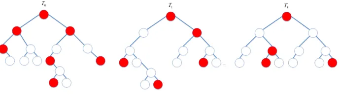
Figure 2 below depicts an M-term (11) selected from an RF ensemble. The red colored nodes illustrate the selection of the M wavelets with the highest norm values from the entire
forest. Observe that they can be selected from any tree at any level, with no connectivity
restrictions.
Figure 2: Selection of an M-term approximation from the entire forest.
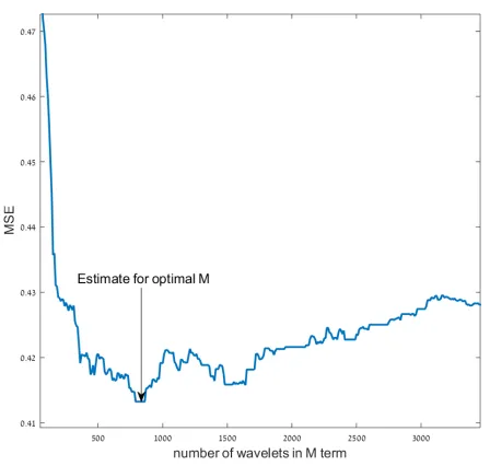
Figure 3 depicts how the parameterM is selected for the challenging “Red Wine Quality”
dataset from the UCI repository (UCI repository). The generation of 10 decision trees on the training set creates approximately 3500 wavelets. The parameter M is then selected by
methods (Loh 2011), using (9), the wavelet approximation method may select significant
components from any tree and any level in the forest. By this method, one does not need to
predetermine the maximal depth of the trees and over-fitting is controlled by the selection of significant wavelet components.
Figure 3: : “Red Wine Quality” dataset - Numeric computation of M for optimal regression.
In a similar manner to certain successful applications in signal processing (e.g. coefficient quantization in the image compression standard JPEG), one may replace the selection of
the parameterM in (11), with a threshold parameterε >0, chosen suitably for the problem
(see for example Section 6.2). One then creates a wavelet approximation using all wavelet terms with norm (6) greater than ε.
In some cases, as presented in (Strobl et. al. 2006) explanatory attributes may be
non-descriptive and even noisy, leading to the creation of problematic nodes in the decision trees. Nevertheless, in these cases, the corresponding wavelet norms are controlled and these nodes
can be pruned out of the sparse representation (11). The following example demonstrates
exactly this, that with high probability, the wavelets associated with the correct variables have relatively higher norms than wavelets associated with non-descriptive variables. Hence
the wavelet based criterion will choose, with high probability the correct variable.
Example 1 Let{yi}mi=1, whereyi∼Ber(1/2)i.i.d. and{xi}mi=1 ⊂[0,1]n, xi = (xi1, . . . , xik, . . . , xin)∈
Rn with xik = yi and xij, j 6= k, uniformly distributed in [0,1]. Then, for a subdivision
1. If j6=k, then kψΩ0k2
2,kψΩ00k2
2 ≤2 log(2/δ),
2. If j=kand the subdivision minimizes (1), then
kψΩ0k2
2,kψΩ00k 2 2 ≥
m
2 − r
log(2/δ) 2m
!3,
m2.
ProofSee Appendix.
4. ‘Weak-Type’ Smoothness and Sparse Representations of the response variable
In this section, we generalize to unstructured and possibly high dimensional datasets, a theoretical framework that has been applied in the context of signal processing, where the
data is well structured and of low dimension (DeVore 1998), (DeVore et. al. 1992).
The ‘sparsity’ of a function in some representation is an important property that provides a robust computational framework (Elad 2010(@). Approximation Theory relates the
sparsity of a function to its Besov smoothness index and supports cases where the function
is not even continuous. Our motivation is to provide additional tools that can be used in the context of machine learning to associate a Besov-index, which is roughly a ‘complexity’ score,
to the underlying function of a dataset. As the theory below and the experimental results
show, this index correlates well with the performance of RFs and wavelet decompositions of RFs.
For a function f ∈ Lτ(Ω), 0 < τ ≤ ∞, h ∈ Rn and r ∈ N, we recall the r-th order
difference operator
∆rh(f, x) := ∆rh(f,Ω, x) :=
r P k=0
(−1)r+k r
k
!
f(x+kh) [x, x+rh]⊂Ω,
0 otherwise,
where [x, y] denotes the line segment connecting any two pointsx, y ∈Rn. The modulus
of smoothness of order r over Ω is defined by
ωr(f, t)τ := sup|h|≤tk∆hr(f,Ω,·)kLτ(Ω), t >0,
where forh∈Rn,|h|denotes the norm of h. We also denote
ωr(f,Ω)τ :=ωr
f,diam(Ω) r
τ
Definition 2 For 0 < p < ∞ and α > 0, we set τ = τ(α, p), to be 1/τ := α + 1/p. For a given function f ∈ Lp(Ω0), Ω0 ⊂Rn, and tree T, we define the associated B-space smoothness in Bα,rτ (T), r∈N, by
|f|Bα,r τ (T):=
X
Ω∈T
|Ω|−αωr(f,Ω)τ τ
!1/τ
, (12)
where, |Ω|denotes the volume of Ω.
We now show that a ‘well clustered’ function is in fact infinitely smooth in the right adaptively chosen Besov space.
Lemma 3 Let f(x) = K P k=
Pk(x)1Bk(x), where each Bk ⊂ Ω0 is a box with sides parallel
to the main axes and Pk ∈Πr−1. We further assume that Bk∩Bj =∅, whenever j 6= k.
Then, there exists an adaptive tree partition T, such that f ∈Bαα,r(T), for anyα >0.
ProofSee Appendix.
For a given forestF ={Tj}Jj=1and weightswj = 1/J, theαBesov semi-norm associated with the forest is
|f|Bα,r τ (F):=
1
J
J X
j=1 |f|τBα,r
τ (Tj)
1/τ
. (13)
The Besov index of f is determined by the maximal index α for which (13) is finite. The
above definition generalizes the classical function space theory of Besov spaces, where the tree partitions are non-adaptive. That is, classical Besov spaces may be defined by the
special case of partitioning into dyadic cubes, each time usingnlevels of the tree.
RemarkAn active research area of approximation theory is the characterization of more geometrically adaptive approximation algorithms by generalizations of the classic ‘isotropic’
Besov space to more ‘geometric’ Besov-type spaces (Dahmen et. al. 2001), (Dekel and Leviatan 2005), (Karaivanov and Petrushev 2003). It is known that different geometric
approximation schemes are characterized by different flavors of Besov-type smoothness. In
this work, for example, we assume all trees are created using partitions along the main n
axes. This restriction may lead in general to potentially lower Besov smoothness of the
underlying function and the sparsity of the wavelet representation. Yet, the theoretical
definitions and results of this paper can also apply to more generalized schemes where for example the tree partitions are by arbitrary hyper-planes. In such a case, the smoothness
Next, for a given tree T and parameter 0 < τ < pwe denote theτ-strength of the tree by
Nτ(f,T) = X
Ω∈T kψΩkτp
!1/τ
. (14)
Observe that
lim
τ→0Nτ(f,T)
τ ={#Ω∈ T :ψ
Ω6= 0}. Let us further denote theτ-strength of a forest F, by
Nτ(f,F) := 1
J
J X
j=1 X
Ω∈Tj
kψΩkτp
1/τ
= 1
J
J X
j=1
Nτ(f,Tj)τ
1/τ
.
In the setting of a single tree constructed to represent a real-valued function, under mild
conditions on the partitions (see remark after (5) and condition (17)) , the theory of (Dekel
and Leviatan 2005) proves the equivalence
|f|Bα,r
τ (T)∼Nτ(f,T). (15)
This implies that there are constants 0< C1 < C2 <∞, that depend on parameters such asα, p, n, r and ρ in condition (17) below, such that
C1|f|Bα,rτ (T)≤Nτ(f,T)≤C2|f|Bα,rτ (T).
Therefore, we also have for the forest model
|f|Bα,r
τ (F) ∼Nτ(f,F). (16)
We now present a “Jackson-type estimate” for the degree of the adaptive wavelet forest approximation. Its proof is in the Appendix.
Theorem 4 Let F ={Tj}Jj=1 be a forest. Assume there exists a constant 0< ρ <1, such
that for any domain Ω ∈ F on a level l and any domain Ω0 ∈ F, on the level l+ 1, with
Ω∩Ω0 6=∅, we have
where |E| denotes the volume of E ⊂ Rn. Denote formally f = P Ω∈F
wj(Ω)ψΩ, and assume
that|f|Bα,r
τ (F)<∞, where
1
τ =α+
1
p.
Then, for the M-term approximation (10) we have
σM(f) :=kf−fMkp ≤C(p, α, ρ)J M −α|f|
Bα,rτ (F) . (18)
One important contribution of this work is the attempt to generalize to the setting of machine learning, the function space theoretical perspective. There are several candidate
numeric methods to estimate the critical ‘weak-type’ Besov smoothness index α from the
given data. That is, the maximal α for which the Besov norm is finite. Our goal is to estimate the true smoothness of the underlying function, removing influences of noise and
outliers if exist within the given dataset. One potential method is to use the equivalence (16)
and then search for a transient value ofτ for whichNτ(f,F) becomes ‘infinite’. However, we choose to generalize the numeric algorithm of (DeVore et. al. 1992) and estimate the
critical indexαusing a numeric exponential fit of the error σM in (18). We found that it is somewhat more robust to fit each decision tree in the forest with an estimated smoothness
index αj and then average to obtain the estimated forest smoothness α. Thus, based on (18), we model the error function byσj,m ∼cjm−αj for unknown cj, αj, where σj,m is the approximation error when using the m most significant wavelets of the jth tree. First,
notice that we can estimatecj ∼σj,1. Then, using RM
1 m
−udm= M1−u−1
(1−u), we estimate αj by
minαj
M1−αj−1
1−αj
σj,1− M−1
X
m=1
σj,m
. (19)
Similarly to (DeVore et. al. 1992), we select only M significant terms, to avoid fitting the
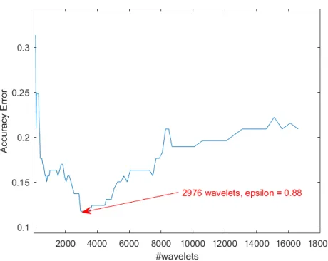
tail of the exponential expression. This is done by discarding wavelets that are overfitting the error on the Out Of Bag (OOB) samples (see Figure 3). Let us see some examples of
how this works in practice. As can be seen in Figure 4, the estimate of the Besov index of two target functions using (19) stabilizes after a relatively small number of trees are added.
Next, we show that when an underlying function is not ‘well clustered’ and has a sharp
transition of values across the boundary of two domains, then the Besov index is limited in the general case and suffers from the curse of dimensionality. Again, it should make sense
to the practitioners, that such a function can be learnt but with more effort, e.g. trees with
higher depth.
Lemma 5 Let f(x) =1Ω˜(x), whereΩ˜ ⊂[0,1]n is a compact domain with a smooth
(a) “Red Wine” (b) “Airfoil”
Figure 4: Estimation of the Besov critical smoothness index
is the tree with isotropic dyadic partitions, creating dyadic cubes of side lengths 2−k on the
level nk.
ProofSee Appendix.
We note that in the general case, when subdivisions along main axes are used, the non-adaptive tree of the above lemma is almost best possible. That is, one cannot hope for
significantly higher smoothness index using an adaptive tree with subdivisions along main
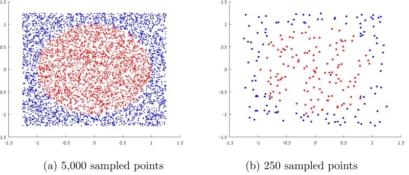
axes. In Figure 5(a) we see 5000 random points and in (b) 250 random points, sampled from a uniform distribution taking a response value off(x) =1Ω˜(x), where ˜Ω⊂R2, is the
unit sphere.
(a) 5,000 sampled points (b) 250 sampled points
By Lemma 4.3, the lower bound for the critical Besov exponent off isα= 0.5, forp= 2.
This should correlate with the intuition of machine learning practitioners: the dataset does
have two well defined clusters, but the boundary between the clusters (boundary of the sphere) is a non-trivial curve and any classification algorithm will need to learn the geometry
of the curve.
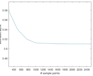
In Figure 6 we see a plot of the numeric calculation of theαBesov index for given number
of sampling points of f. We see relatively fast convergence toα= 0.51. As discussed, our method attempts to capture the geometric properties of the ‘true’ underlying function that
is potentially buried in the noisy input data. To show this, we constructed from a dataset
of 10k samples of f, a ten dimensional dataset, by adding additional eight noisy features, with uniform distribution in [0,1] and no bearing on the response variable. The numeric
computation in this example was again,α = 0.51, which demonstrates that the method is
stable under this noisy embedding in Rn as well.
Figure 6: Numeric calculation of the αBesov index for given number of sampling points of the indicator function of a unit sphere.
5. Wavelet-based variable importance
In many cases, there is a need to understand in greater detail in what way the different
variables influence the response variable (Guyon and Elisseff 2003). Which of the possibly hundreds of parameters is more critical? What are the interactions between the significant
variables? Also, the property of obtaining fewer features that provide equivalent prediction
could be used for feature engineering and for ‘feature budget algorithms’ such as in (Feng et. al. 2015), (Vens and Costa 2011). As described in (Genuer et. al. 2010), the use of
There are several existing Variable Importance (VI) quantification methods that use
RF. A popular approach for measuring the importance of a variable is summing the total
decrease in node impurities when splitting on the variable, averaged over all trees (RF in R), (Hastie et. al. 2009). As suggested in the RF package documentation of the R language (RF
in R): “For classification, the node impurity is measured by the Gini Index. For regression;
it is measured by the residual sum of squares”. Although not stated specifically in (RF in R), it is common practice to multiply the information gain of each node by its size (Raileanu
and Stoffel 2004), (Du and Zhan 2002), (Rokach and Maimon 2005). Additional methods
for variable importance measure are the ‘Permutation Importance’ measure (Genuer et. al. 2010), or similarly ‘OOB randomization’ (Hastie et. al. 2009). With these latter
two methods, sequential predictions of RF are done, when each time one feature is being
permuted as the rest of the features remain. Then, the measure for variable importance is the difference in prediction accuracy before and after a feature is permuted in MSE terms.
However, both ‘Impurity gain’ and ‘Permutation’ have some pitfalls that should be
considered, when used for variable importance. As shown by (Strobl et. al. 2006), the
‘Impurity gain’ tends to be in favor of variables with more varying values. As shown in (Strobl et. al. 2008), ‘Permutation’ tends to overestimate the variable importance of highly
correlated variables.
The wavelet-based VI is derived by imposing a restriction on the adaptive re-ordering
of the wavelet components (11), such that they must appear in ‘feature related blocks’. To make this precise, let{x∈Rn, f(x)}be a dataset and let ˜frepresent the RF decomposition,
as in (8). We evaluate the importance of thei-th feature by
Sτi := 1
J
J X
j=1 X
Ω∈Tj∩Vi
kψΩkτ2, i= 1, . . . , n, (20)
where, τ >0 andVi is the set of child domains formed by partitioning their parent domain along the ith variable. This allows us to score the variables, using the ordering Sτ
i1 ≥
Siτ
2 ≥ · · ·. Recall that our wavelet-based approach transforms classification problems into the functional setting (see section 2) by mapping each label lk to a vertex~lk ∈RL−1 of a
regular simplex. Therefore, in classification problems, the wavelet norms in (20) are given
by (7) which implies that we provide a unified approach to VI.
It is crucial to observe that from an approximation theoretical perspective, the more
the variables by the approximation error of their corresponding wavelet subset
min1≤i≤n ˜
f− 1
J
J X
j=1 X
Ω∈Tj∩Vi
ψΩ 2
= min1≤i≤n 1 J X
k6=i J X
j=1 X
Ω∈Tj∩Vk
ψΩ 2 ≤min1≤i≤n
1
J
X
k6=i J X
j=1 X
Ω∈Tj∩Vk
kψΩk2
= min1≤i≤n X
k6=i
Sk1
= X
1≤k≤n
Sk1−max1≤i≤nSi1.
What is interesting is that, in regression problems, when using piecewise constant
approxi-mation in (1),(4), the VI score (20) withτ = 2, is in fact exactly as in (Louppe et. al. 2013) when variance is used as the impurity measure. To see this, for any dataset{x∈Rn, f(x)} and domain ˜Ω of an RF, denote briefly
KΩ˜ := # n
xi ∈Ω˜ o
, VarΩ˜= 1 #nxi ∈Ω˜
o X
xi∈Ω˜
f(xi)−CΩ˜ 2
.
For any domain Ω of a RF, with children Ω0,Ω00, the variance impurity measure is
∆ (Ω) :=Var (Ω)−KΩ0
KΩ
Var Ω0− KΩ00
KΩ
Var Ω00.
The importance of the variablei(up to normalization by the size of the dataset) is defined
in (Louppe et. al. 2013) by
1 J J X j=1 X
children ofΩinTj∩Vi
KΩ∆ (Ω). (21)
Theorem 6 The variable importance methods of (20) and (21) are identical forτ = 2.
Proof For any domain Ω and its two children Ω0,Ω00,
KΩ∆ (Ω) =KΩ
Var (Ω)−KΩ0
KΩ
Var Ω0−KΩ00
KΩ
Var Ω00
= X xi∈Ω
(f(xi)−CΩ)2− X
xi∈Ω0
(f(xi)−CΩ0)2−
X
xi∈Ω00
(f(xi)−CΩ00)2
Therefore,
1
J
J X
j=1
X
children ofΩinTj∩Vi
KΩ∆ (Ω) =Si2.
♦
Further to the choice of τ = 1 over τ = 2 in (20), the novelty of the wavelet-based VI approach is targeted at difficult noisy datasets. In these cases, one should compute VI at
various degrees of approximation, using only subsets of ‘significant’ nodes, by thresholding
out wavelet components with norm below some ε >0
Si1(ε) := J X
j=1
X
Ω∈Tj∩Vi,kψΩk≥ε
kψΩk2. (22)
As pointed out, a popular RF approach for identifying important variables is summing the
total decrease in node impurities when splitting on the variable, averaged over all trees
(RF in R), (Hastie et. al. 2009). However, this method may not be reliable in situations where potential predictor variables vary in their scale of measurement or their number of
categories (Strobl et. al. 2006). This restriction is very limiting in practice, as in many cases binary variables such as ‘Gender’ are very descriptive where less descriptive variables
(or noise) may vary with many values.
To demonstrate this problem, we follow the experiment suggested in (Strobl et. al.
2006). We set a number of samples tom= 120, where each sample has two explanatory
in-dependent variables: x1∼N(0,1) and x2 ∼Ber(0.5). A correlation betweeny=f(x1, x2) and x2 is established by:
y ∼ (
Ber(0.7), x2 = 0,
Ber(0.3), x2 = 1. )
(23)
In accordance with the point made in (Strobl et. al. 2006), when applying the VI of (RF in R), (Hastie et. al. 2009) we observe that the important variable is the ‘noisy’
uncorre-lated feature x1. As shown in Example 1, while we may obtain many false partitions along the noise, with high probability their wavelet norm is controlled, and relatively small. In Figure 7 we see a histogram of the wavelet norms (taken from one of the RF trees) for the
example (23). We see that the wavelet norms of the important variable x2 are larger, but that there exists a long tail of wavelet norms relating tox1. Therefore, applying the thresh-olding strategy (22) as part of the feature importance estimation could be advantageous in
such a case.
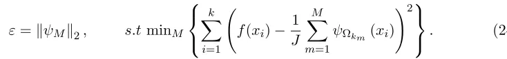
We now address the choice of in (22). So as to remove the noisy wavelet components
Figure 7: wavelets norms taken from one of the RF trees constructed for the example (23)
M is the selected using theM-term wavelet that minimizes the approximation error on the
validation set{xi, f(xi)}i=1,..k by
ε=kψMk2, s.t minM
k X
i=1
f(xi)− 1
J
M X
m=1
ψΩkm(xi)
!2
. (24)
The calculation of for the “Pima diabetes” dataset using a validation set is depicted in Figure 8. In Section 6.2 we demonstrate the advantage of the wavelet-based thresholding
technique in VI on several datasets.
6. Applications and Experimental Results
For our experimental results, we implemented C# code that supports RF construction, Besov index analysis, wavelet decompositions of RF and applications such as wavelet-based
VI, etc. (source code is available, see link in (Wavelet RF code)). The algorithms are
executed on the Amazon Web Services cloud, using up to 120 CPUs. Most datasets are taken from the UCI repository (UCI repository), which allows us to compare our results
Figure 8: “Pima diabetes” - Choice of in (22) using the validation set
6.1 Ensemble Compression
In applications, constructed predictive models, such as RF, need to be stored, transmitted
and applied to new data. In such cases the size of the model becomes a consideration, especially when using many trees to predict large amounts of incoming new data over
distributed architectures. Furthermore, as presented in (Geurts and Gilles 2011), the
number of total nodes of the RF and the average tree depth impact the memory requirements and evaluation performance of the ensemble.
In order to demonstrate the correlation between the Besov index of the underlying
function and the ‘complexity’ of these datasets we need to compare on the same scale different datasets of different sizes and dimensions. Therefore, we replaced the commonly
used metrics in machine learning such as MSE (Mean Square Error) by the normalized
PSNR (Peak Signal To Noise Ratio) metric which is commonly used in the context of signal processing. For a given dataset {xi, f(xi)} and an approximation {xi, fA(xi)} PSNR is defined by
PSNR:=10·log10 maxi,j
n
|f(xi)−f(xj)|2 o
1 #{xi}
P
i(f(xi)−fA(xi)) 2.
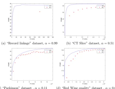
Observe that higher PSNR implies smaller error. In Figure 9 we observe the rate-distortion
performance measured on validation points in a fivefold cross validation ofM−termwavelet approximation and standard RF, as trees are added. It can be seen that for functions that are smoother in ‘weak-type’ sense (e.g. higher α), wavelet approximation outperforms the
(a) “Record linkage” dataset,α= 0.99 (b) “CT Slice” dataset, α= 0.51
(c) “Parkinson” dataset , α= 0.11 (d) “Red Wine quality” dataset ,α= 0.07
We now compare wavelet-based compression with existing RF pruning strategies. As
stated by (Kulkarni and Sinha 2012), most of the current efforts in pruning RF are based on
‘Over-produce-and-Choose’ strategy, where the forest is grown to a fixed number of trees, and then only a subset of these trees are chosen by a ‘leave one out strategy’ as in
(Martinez-Muoz et. al. 2009), (Yang et. al. 2012). For each dataset we first computed a point at
which the graph of wavelet approximation error begins to ‘flatten out’ on the validation set. We then used this target error pre-saturation point for both wavelet shrinkage and
the pruning methods that aim for a minimal number of nodes to achieve it on a validation
set of fivefold cross validation. To this end, we have generated RF with 100 decision trees with 80% bagging and √n hyper-parameter. The two pruning strategies are based on a ‘leave one out’ strategy as presented in (Yang et. al. 2012). In this approach trees are
recursively omitted according to their correspondence with the rest of the ensemble (based on the correspondence of the margins in classification and MSE in regression). We have
collected the results of the experiment described above applied to 12 UCI datasets in Table
1. The datasets for classification are marked (C) and regression (R). One may observe from Table 1 that the wavelet-based method performs better than conventional pruning. Also,
as expected, there is significant correlation between the performance of compression and the function smoothness. That is, the compression is more effective for smoother functions.
Note that when computing anM-term wavelet approximation, some components may be
unconnected as depicted in Figure 2. Obviously, any compression of the wavelet approxima-tion would need to encode the nodal data associated with these unconnected components.
Therefore, we enforce connectivity on any wavelet approximation we compute, by adding
all wavelet components along the tree paths leading to the selected significant wavelet com-ponents. Thus, the wavelet compression appearing in Table 1 is in the form of a collection
of J connected subtrees.
6.2 Variable Importance
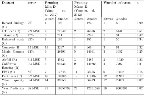
We first demonstrate how the wavelet-based method (20) withτ = 1, succeeds in identifying the features with the highest impact on the prediction. In Figure 10 (a), we show an
histogram of VI scores for the “Red Wine” dataset using the wavelet-based approach (20).
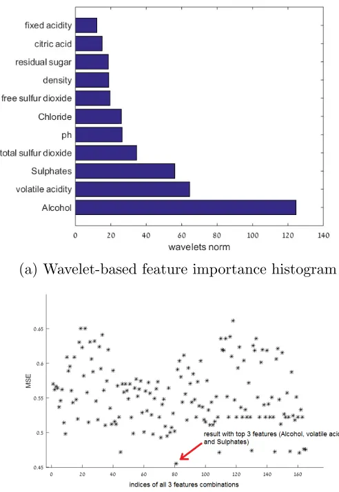
As can be seen, the top three features in the histogram are ‘Alcohol’, ‘Volatile acidity’ and ‘Sulphates’. We then constructed RFs for all the possible triple combinations of features
of the UCI repository ‘Wine Quality’ dataset (165 simulations) using 100 trees and 80%
bagging. In Figure 10(b), we can see the MSE of each of these RFs. One can verify that the triple ‘Alcohol’, ‘Volatile acidity’ and ‘Sulphates’ (index 81) has the smallest error, as
Table 1: Compression - number of nodes required to reach the error pre-saturation point
Dataset error Pruning
Min-D (Yang et. al. 2012)
Pruning Mean-D (Yang et. al. 2012)
Wavelet subtrees α
#trees #nodes #trees #nodes #trees #nodes Record linkage
(C)
2% 1 123 1 123 1 6 0.99
CT Slice (R) 2.9 MSE 2 77042 2 76396 2 5141 0.51
Titanic (C) 17% 3 711 10 2248 1 34 0.42
Balanced scale (C)
22% 1 185 1 185 1 55 0.34
Concrete (R) 15 MSE 19 2297 8 966 3 64 0.32
Magic Gamma (C)
13% 9 26793 5 14961 3 1657 0.25
Airfoil (R) 3.2 MSE 5 4533 3 7487 3 1929 0.23
California Housing (R)
0.5 MSE 4 65436 9 149863 4 7292 0.2
EEG (C) 8% 7 17845 11 28355 6 12808 0.15
Parkinson (R) 3.2 MSE 18 103822 19 110187 12 20947 0.11 Wine quality
(R)
0.4 MSE 14 39350 13 36439 12 29089 0.07
Year Prediction (R)
(a) Wavelet-based feature importance histogram
(b) Error of RFs constructed over all possible 3 feature subsets
Next, we show that the wavelet-based VI approach, in particular, the noise-removal
variant using (22) with > 0, can provide a better estimation of VI than the existing
methods in R (RF in R). Note that we apply the wavelet-based VI method in classification problems as well, competing with, for example, the standard Gini-based algorithm of R.
To this end we employ a test methodology used in (Feng et. al. 2015). Using each VI
method we first calculate a corresponding VI score of the features. Each method uses an RF with 100 trees and 80% bagging. However, the wavelet-based method was computed
using our implementation, based on (22) while the Permutation and Information Gain based
methods were applied using R. After each method ‘decides’ on the order of the features by importance, we iterate by adding features one-by-one, where at thek-th iteration, only the
selected first kfeatures are used for prediction. Here also, we used wavelet-based choice of
kmost important features to construct a wavelet-based best prediction, while for the other methods, we used their choice ofkmost important features as the input for an R based RF.
The results of fivefold cross validation are presented in Figure 11. For example, in Figure
11(a), we see that on the “Parkinson” dataset, the wavelet-based method reaches better prediction using the first three features it selected. This is due to fact that the wavelet-based
method selected different features (‘Age’, ‘Time’ and ‘Gender’) than the other methods.
6.3 Classification and regression tasks
In this Section we focus on difficult datasets, such as small sets or with high bias, bad features, mis-labeling and outliers (see for example “Pima Diabetes” dataset with only 768
samples with 8 attributes in Figure 11(c)) and show that in such cases the wavelet-based
approach provides smaller predictive errors.
We begin with a demonstration of a case of ‘false labeling’ using the R machine learning
benchmark “Spirals” (Spiral dataset). From the given dataset we create a dataset with
mis-labeling by randomly replacing 20% of the values of the response variable. The original and noisy datasets are rendered in Figure 12. We then compare the predictive performance of
the standard RF and theM-term wavelet approximation (11), where optimalM values are
computed automatically as depicted in Figure 3. We also compare the M-term performance to a minimal node size restriction as in (Biau and Scornet 2016), setting this value to 5,
as in (Denil et. al. 2014). We perform RF construction with 1000 trees and 5 fold cross
validation.
When the training dataset contains ‘false labeling’, the correspondence with the testing
set is reduced. Trying to restrict the tree depth, can potentially miss the geometry of the
underlying function, while too many levels can lead to overfitting. As seen in Table 2, the wavelet approach selects the right significant components from any tree and any level and
(a) “Parkinson” dataset, = 1.74.
(b) “Magic gamma” dataset, = 0.57.
(c) “Pima Diabetes” dataset,= 0.93.
(a) Original set (b) Set with amplified mis-labeling
Figure 12: ‘Spirals’ dataset (Spiral dataset)
approach is more significant in the second case with more ‘false labeling’ in the training set.
Table 2: ‘Spirals’ dataset - Classification results.
Wavelet error RF error Pruned RF error Original spiral set 12.2±0.9% 14.4±1.1% 15.9±0.8% Set with amplified
mis-labeling
13.9±1.2% 17.8±1.3% 22.7±1.6%
Next, we compare the performance of wavelet-based regression with state-of-the-art method on a challenging problem. The authors of (Denil et. al. 2014) provide comparative
results of different pruning strategies for the difficult “Wine Quality” dataset. Learning this
dataset is challenging since the data is very biased and depends on the personal taste of the wine experts. In Table 3 below, we collect the results of (Biau 2012), (Biau et. al. 2008),
(Breiman 2001) and (Denil et. al. 2014) (as listed in (Denil et. al. 2014)). The RFs are
all constructed of 1000 trees and fivefold cross validation is applied. We follow the notation presented in (Denil et. al. 2014) and use the abbreviation that was provided for each
method variation (‘+’,’F’,’S’,’NB’, ‘T’). In our RF implementation, we used bootstrapping
with 80% and randomized√nfeatures at each node. M was selected automatically using 10 percent of the training set.
Another form of a challenging dataset is when some of the features are extremely noisy or uncorrelated with the response variable. As shown in (Strobl et. al. 2006) (see the
discussion in Section 5), in such cases, RF partitions sometimes are influenced by these
variables and the constructed ensemble is of lower quality. To explore the impact of our approach on such datasets, we used the “Poker Hand” dataset from the UCI repository
Table 3: Performance comparison on the “Wine Quality” Algorithm MSE
Biau08 0.53
Biau12 0.59
Biau12+T 0.57
Biau12+S 0.57
Denil 0.48
Denil+F 0.48
Denil+S 0.41
Breiman 0.4
Breiman+NB 0.39 Wavelets 0.36
id”. As can be seen from Figure 13, the wavelet method significantly outperforms the
standard RF regression, especially in the second scenario with the ‘bad’ feature included.
(a) ‘Bad’ feature excluded (b) ‘Bad’ feature included
Figure 13: The impact of a bad feature on the regression of the “Poker Hand” dataset
The authors would like to thank the reviewers for their careful reading of several versions
of this work and valuable comments which resulted in a substantially revised manuscript.
This work was supported by an ‘AWS in Education Grant award’.
References
Alani D., Averbuch A. and Dekel S., Image coding using geometric wavelets, IEEE
trans-actions on image processing 16:69-77, 2007.
Alpaydin E.,Introduction to machine learning, MIT Press, 2004.
Avery M., Literature Review for Local Polynomial Regression,
http://www4.ncsu.edu/ mravery/AveryReview2.pdf.
Bernard S., Adam S. and Heutte L., Dynamic random forests, Pattern Recognition Letters
33:1580-1586.
Biau G., Analysis of a random forests model, Journal of Machine Learning Research 13:
1063-1095, 2012.
Biau G., Devroye L. and Lugosi G., Consistency of random forests and other averaging
classifiers, Journal of Machine Learning Research 9:2015-2033, 2008.
Biau G. and Scornet E., A random forest guided tour,TEST 25(2):197-227, 2016.
Breiman L., Random forests, Machine Learning 45:5-32, 2001.
Breiman L., Bagging predictors,Machine Learning 24(2):123-140, 1996.
Breiman L, Friedman J., Stone C. and Olshen R., Classification and Regression Trees,
Chapman and Hall/CRC, 1984.
Boulesteix A., Janitza S., Kruppa J. and K¨onig I., Overview of random forest methodology and practical guidance with emphasis on computational biology and bioinformatics,Wiley
Interdisciplinary Reviews: Data Mining and Knowledge Discovery 2(6):493-507, 2012.
Chen H., Tino P. and Yao X., Predictive Ensemble Pruning by Expectation Propagation,
IEEE journal of knowledge and data engineering 21:999-1013, 2009.
Christensen O., An introduction to Frames and Riesz Bases, Birk¨auser, 2002.
Criminisi A., Shotton J. and Konukoglu E., Forests for Classification, Regression, Den-sity Estimation, Manifold Learning and Semi-Supervised Learning, Microsoft Research
Dahmen W., Dekel S. and Petrushev P., Two-level-split decomposition of anisotropic Besov
spaces, Constructive approximation 31:149-194, 2001.
Daubechies I.,Ten lectures on wavelets, CBMS-NSF Regional Conference Series in Applied
Mathematics,1992.
Dekel S., Gershtansky I., Active Geometric Wavelets, In Proceedings of Approximation
Theory XIII 2010, 95-109, 2012.
Dekel S. and Leviatan D., Adaptive multivariate approximation using binary space
parti-tions and geometric wavelets, SIAM Journal on Numerical Analysis 43:707-732, 2005.
Denil M., Matheson D. and De Freitas N., Narrowing the gap Random forests in theory and in practice, In Proceedings of the 31st International Conference on Machine Learning 32,
2014.
DeVore R., Nonlinear approximation,Acta Numerica 7:51-150, 1998.
DeVore R. and Lorentz G., Constructive approximation, Springer Science and Business, 1993.
DeVore R., Jawerth B. and Lucier B., Image compression through wavelet transform coding,
IEEE transactions on information theory 38(2):719-746, 1992.
Du W. and Zhan Z., Building decision tree classifier on private data, In Proceedings of the IEEE international conference on Privacy, security and data mining 14:1-8, 2002.
Elad M., Sparse and redundant representations: from theory to applications in signal and
image processing, Springer Science and Business Media, 2010.
Feng N., Wang J. and Saligrama V., Feature-Budgeted Random Forest, In Proceedings of
The 32nd International Conference on Machine Learning, 1983-1991, 2015.
Kelley P. and Barry R., Sparse spatial autoregressions, Statistics and Probability Letters
33(3):291-297, 1997.
Gavish M., Nadler B., Coifman R., Multiscale wavelets on trees, graphs and high
dimen-sional data: Theory and applications to semi supervised learning, In Proceedings of the 27th International Conference on Machine Learning, 367-374, 2010.
Genuer R., Poggi J. and Christine T., Variable selection using Random Forests, Pattern
Geurts P. and Gilles L., Learning to rank with extremely randomized trees, In JMLR:
Workshop and Conference Proceedings 14:49-61, 2011.
Guyon I. and Elisseff A., An introduction to variable and feature selection, Journal of
Machine Learning Research 3:1157-1182, 2003.
Hastie T., Tibshirani R. and Friedman J., The elements of statistical learning, Springer,
2009.
Joly A., Schnitzler F.,Geurts P. and Wehenkel L., L1-based compression of random for-est models, In Proceedings of the European Symposium on Artificial Neural Networks,
Computational Intelligence and Machine Learning, 375-380, 2012.
Karaivanov B. and Petrushev P., Nonlinear piecewise polynomial approximation beyond
Besov spaces, Applied and computational harmonic analysis 15:177-223, 2003.
Kulkarni V. and Sinha P., Pruning of Random Forest classifiers: A survey and future
directions, In International Conference on data science and engineering, 64-68, 2012.
Lee A., Nadler B. and Wasserman L., Treelets: an adaptive multi-scale basis for sparse unordered data, Annals of Applied Statistics 2(2):435-471, 2008.
Loh W., Classification and regression trees,Wiley Interdisciplinary Reviews: Data Mining
and Knowledge Discovery 1(1):14-23, 2011.
Louppe G., Wehenkel L., Sutera A. and Geurts P., Understanding variable importances in
forests of randomized trees, Advances in Neural Information Processing Systems 26:431-439, 2013.
Mallat S.,A Wavelet tour of signal processing, 3rd edition (the sparse way), Acadmic Press, 2009.
Martinez-Muoz G., Hern´andez-Lobato D. and Suarez A., An analysis of ensemble pruning
techniques based on ordered aggregation, IEEE Transactions on pattern analysis and
machine intelligence 31:245-259, 2009.
Radha H., Vetterli M. and Leonardi R., Image compression using binary space partitioning trees, IEEE transactions on image processing 5:1610-1624, 1996.
Raileanu L. and Stoffel K., Theoretical comparison between the Gini index and information gain criteria, Annals of Mathematics and Artificial Intelligence 41(1):77-93, 2004.
‘Random Forest’ package in R,
Rokach L. and Maimon O., Top-down induction of decision trees classifiers-a survey,IEEE
transactions on systems, man, and cybernetics, part C: applications and reviews
35(4):476-487, 2005.
Salembier P. and Garrido L., Binary partition tree as an efficient representation for image
processing, segmentation, and information retrieval,IEEE transactions on image
process-ing9:561-576, 2000.
Spiral dataset,
http://www.inside-r.org/packages/cran/mlbench/docs/mlbench.spirals.
Strobl C., Boulesteix A., Zeileis A. and Hothorn T., Bias in random forest variable
impor-tance measures, In Workshop on Statistical Modelling of Complex Systems, 2006.
Strobl C., Boulesteix A., Kneib T., Augustin T. and Zeileis A., Conditional variable
impor-tance for random forests, BMC bioinformatics 9(1):1-11, 2008.
UCI machine learning repository, http://archive.ics.uci.edu/ml/.
Vens C. and Costa F., Random forest based feature induction, InIEEE international
con-ference on data mining, 744-753, 2011.
Yang F.,Lu. W., Luo L. and Li T., Margin optimization based pruning for random forest,
Neurocomputing 94:54-63, 2012.
Wavelet-based Random Forest source code, https://github.com/orenelis/WaveletsForest.git.
Appendix
Denoting briefly for any domain ˜Ω, KΩ˜ := # n
xi ∈Ω˜ o
we have
X
xi∈Ω
(f(xi)−CΩ)2−VΩ= X
xi∈Ω
(f(xi)−CΩ)2− X
xi∈Ω0
(f(xi)−CΩ0)2−
X
xi∈Ω00
(f(xi)−CΩ00)2
= X xi∈Ω0
h
(f(xi)−CΩ)2−(f(xi)−CΩ0)2
i +
X
xi∈Ω00
h
(f(xi)−CΩ)2−(f(xi)−CΩ00)2
i
= 2 (CΩ0−CΩ)
X
xi∈Ω0
f(xi) +KΩ0 CΩ2 −CΩ20
+ 2 (CΩ00−CΩ)
X
xi∈Ω00
f(xi) +KΩ00 C2
Ω−CΩ200
= 2 (CΩ0−CΩ)KΩ0CΩ0+KΩ0 CΩ2 −C2
Ω0
+ 2 (CΩ00−CΩ)KΩ00CΩ00+KΩ00 CΩ2 −C2
Ω00
=KΩ0(CΩ0 −CΩ)2+KΩ00(CΩ00−CΩ)2
=kψΩ0k2
2+kψΩ00k 2
2 =WΩ. Now, since P
xi∈Ω
(f(xi)−CΩ)2is independent of the selection of the partition of Ω and since
WΩ is always positive, the search for minimizingVΩ is equivalent to maximizing WΩ. ♦
Proof of Example 1
1. For any attribute j 6=k we denote m1 := #{xi ∈Ω0} and m2 := m−m1. Hence, for any δ∈(0,1), applying the Hoeffding bound gives w.p. ≥1−δ
CΩ0 −1
2 ≤ s
log(2/δ) 2m1
,
CΩ00−1
2 ≤ s
log(2/δ) 2m2
. (25)
Note, that we can write CΩ = mm1CΩ0+m2
mCΩ00. Thus, using (25) we get w.p. ≥1−δ (CΩ−CΩ0)2 = m
2 2
m2 (CΩ00−CΩ0) 2 ≤ m 2 2 m2 1 m1 + 1 m2
Therefore, w.p. ≥1−δ,
kψΩ0k2
2=m1(CΩ−CΩ0)2
≤ m1m 2 2 m2 1 m1 + 1 m2
log (2/δ)
=
m22 m2 +
m1m2
m2
log (2/δ)
≤2 log (2/δ).
2. Observe that for the case j =k, a subdivision that minimizes (1) is xk = 1/2. Denote
m1 = #{xi ∈Ω : yi = 1}. Applying the Hoeffding bound with δ ∈ (0,1) yields w.p. ≥1−δ
m1−
m 2 ≤ r
log(2/δ) 2m .
If Ω0 is the subset of [0,1]n where xk > 1/2, then CΩ0 = 1 and kψΩ0k2
2 = m1 1− m1
m 2
. Plugging into the bound above we conclude that w.p. ≥1−δ,
kψΩ0k2
2 ≥
m
2 − r
log(2/δ) 2m ! 1− m 2 + q log(2/δ)
2m m 2 = m 2 − r
log(2/δ) 2m
!3,
m2.
♦
Proof of Theorem 4 We prove the case 1 < p <∞ (the case 0 < p ≤1 is easier). We need to show two essential properties. First, for any Ω0 ∈ F and any x ∈ Ω0, denoting Λ :={Ω∈ F :x∈Ω,|Ω| ≥ |Ω0|}, we have
X
Ω∈Λ
|Ω0| |Ω|
1/p
≤C(ρ, p)J. (26)
Indeed, using (17), recursively for all domains on lower levels intersecting with Ω0 we have
X
Ω∈Λ |Ω0|
|Ω| 1/p ≤ ∞ X k=0
J ρk/p
Secondly, we need the property that
kψΩk∞≤c|Ω| −1/pk
ψΩkp , ∀Ω∈ F. (27)
It is easy to see property (27) for the caser = 1, whereψΩ=1ΩCΩ, but it is also known for the general case of r ≥1 and convex domains (see e.g (Dekel and Leviatan 2005)). This allows us to prove the following Lemma
Lemma 7 For 1< p <∞, let F(x) = I P i=1
wj(Ωi)ψΩi(x),Ωi ∈ F, where
wj(Ω
i)ψΩi
p ≤L.
Then
kFkp ≤cJ LI1/p. (28)
Proof Applying property (27) gives
kFkp ≤ I X i=1
wj(Ωi)ψΩi
∞1Ωi(·) p ≤L I X i=1
|Ωi|−1/p1Ωi(·)
p . We define
Γ (x) := (
min1≤i≤I{|Ωi|:x∈Ωi}, x∈SIi=1Ωi,
0, else.
Then, (26) yields
I X
i=1
|Ωi|−1/p1Ωi(x)≤cJΓ (x)
−1/p
, ∀x∈Ω0.
Thus,
kFkp ≤cL
Γ (·) −1/p p
=cJ L
Z
S
Ωi
Γ (x)−1dx
!1/p
≤cJ L
I X
i=1 |Ωi|−1
Z
Ωi
dx
!1/p
=cJ LI1/p.
We now proceed with the proof of the Theorem. Observe that we may use (16), that is, |f|Bα,r
τ (F)∼Nτ(f,F). Forν = 1,2,· · · , denote
Ξν := n
Ω∈ F: 2−νNτ(f,F)≤wj(Ω)kψΩkp <2 −ν+1N
τ(f,F) o
.
Recall that for any non-negative discrete sequence β ={βk}∞k=1, the weak-lτ norm kβkwlτ, is defined as the infimum (if exists) over all A >0, for which
#{βk:βk> ε}ετ ≤Aτ, ∀ε >0.
Since kβkwl
τ ≤ kβklτ, this implies that
#Ξm ≤ X
ν≤m
#Ξν = # [
ν≤m
Ξν ≤2mτ.
LetFν(x) := P Ω∈Ξν
wj(Ω)ψΩ(x). For the special case M := P ν≤m
#Ξν, we have by (28)
kf−fMkp ≤ ∞ X
ν=m+1
Fν p ≤ ∞ X
ν=m+1 kFνkp
≤cJ
∞ X
ν=m+1
2−νNτ(f,F) (#Ξν)1/p
≤cJNτ(f,F) ∞ X
ν=m+1
2−ν(1−τ /p)
≤cJNτ(f,F)M−(1/τ−1/p)=cJNτ(f,F)M−α.
Extending this result for any M ≥ 1 is standard (using a larger leading constant). This completes the proof.
♦
Proof of Lemma 3 Since there are a finite number of boxes, there exists a, possibly unbalanced, binary tree that after at most K2n partitions, has also the boxes {Bk} as nodes of the tree. Since the modulus of smoothness of orderr of polynomials of degreer−1 is zero (DeVore 1998), (Devore and Lorentz 1993), for any of these box nodes we have that
Similarly, for any descendant node Ω0 ⊂Bk, for some 1≤k≤K,
ωr f,Ω0
τ =ωr Pk,Ω 0
τ = 0.
For any node Ω such that Ω∩Bk=∅, 1≤k≤K, we have
ωr(f,Ω)τ =ωr(0,Ω)τ = 0.
We may then conclude that ωr(f,Ω)τ 6= 0, for only a finite low-level subset Λ of the tree nodes, each strictly containing at least oneBk. Therefore, for any α >0,
|f|Bα,r τ =
X
Ω∈T
|Ω|−αωr(f,Ω) τ
!1/τ
= X
Ω∈Λ
|Ω|−αωr(f,Ω)τ τ
!1/τ
≤2rkfkτ
min k |Bk|
−α
(K2n)1/τ,
where we have used the inequality
ωr(f,Ω)τ ≤2rkfkLτ(Ω)≤2
rkfk Lτ(Ω0).
♦
Proof of Lemma 5As stated, the treeTI with isotropic dyadic partitions, creates dyadic cubes of side lengths 2−k at the level nk. Let us denote by D:={Dk}∞k=0, the collection of dyadic cubes of [0,1]n, whereDk is the collection of cubes with side lengths 2−k. Observe that any domain Ω0 ∈ TI, at a level nk < l < n(k+ 1), is contained in some dyadic cube Ω ∈ T ∩Dk at the level nk. Also, from the properties of the modulus of smoothness, Ω0 ⊂Ω⇒ωr(f,Ω0)τ ≤ωr(f,Ω)τ. Combining these two observations gives
Ω0
−α
ωr f,Ω0
τ ≤2
nα|Ω|−αω
r(f,Ω)τ.
Next, observe that for any Ω∈Dk
ωr(f,Ω)τ (
= 0, Ω∩∂Ω =˜ ∅,
where∂Ω is the boundary of ˜˜ Ω. Therefore,
|f|Bα,r
τ (T)≤c(n, α, τ)
X
Ω∈D
|Ω|−αωr(f,Ω)τ τ
!1/τ
≤c(n, α, τ, r) ∞ X
k=0
2kn(ατ−1)#nΩ∈Dk: Ω∩∂Ω˜ 6=∅ o
!1/τ
.
Thus, it remains to estimate the maximal number of dyadic cubes of side length 2−k that can intersect a smooth boundary of a domain ˜Ω ⊂ [0,1]n. For sufficiently large k, only one connected component of the boundary ∂Ω intersects a dyadic cube Ω˜ ∈Dk, in similar manner to an hyperplane of dimensionn−1 with surface area ≤c2−k(n−1). Therefore, for sufficiently largek
# n
Ω∈Dk: Ω∩∂Ω˜ 6=∅ o
≤c2k(n−1).
This gives
|f|Bα,r τ (T)≤c
n, α, τ, r, ∂Ω˜ X∞
k=0
2kn(ατ−1)2k(n−1) !1/τ
.
Therefore, if τ−1=α+ 1/p, then
α < 1
p(n−1) ⇒ |f|Bα,τ 1(T)<∞.