The Factorized Self-Controlled Case Series Method: An Approach for Estimating the Effects of Many Drugs on Many Outcomes

The Factorized Self-Controlled Case Series Method: An

Approach for Estimating the Effects of Many Drugs on

Many Outcomes

Ramin Moghaddass [email protected]

Department of Industrial Engineering University of Miami

Coral Gables, FL, USA

Cynthia Rudin [email protected]

Department of Computer Science

Department of Electrical and Computer Engineering Duke University

Durham, NC, USA

David Madigan [email protected]

Department of Statistics Columbia University New York, NY, USA

Editor:Benjamin M. Marlin, C. David Page, and Suchi Saria

Abstract

We provide a hierarchical Bayesian model for estimating the effects of transient drug ex-posures on a collection of health outcomes, where the effects of all drugs on all outcomes are estimated simultaneously. The method possesses properties that allow it to handle important challenges of dealing with large-scale longitudinal observational databases. In particular, this model is a generalization of the self-controlled case series (SCCS) method, meaning that certain patient specific baseline rates never need to be estimated. Further, this model is formulated with layers of latent factors, which substantially reduces the num-ber of parameters and helps with interpretability by illuminating latent classes of drugs and outcomes. We believe our work is the first to consider multivariate SCCS (in the sense of multiple outcomes) and is the first to couple latent factor analysis with SCCS. We demon-strate the approach by estimating the effects of various time-sensitive insulin treatments for diabetes.

Keywords: Bayesian Analysis, Drug Safety, Self-Controlled Case Series, Matrix Factor-ization, Effect Size Estimation

1. Introduction

opportunities to add to the evidence base concerning these issues, though the complexity and scale of some of the available databases presents interesting statistical and computational challenges. In what follows we focus on using longitudinal observational databases to make inference about the effects of many drugs with respect to many outcomes simultaneously.

Many research studies have attempted to characterize the relationship between time-varying drug exposures and adverse events (AEs) related to health outcomes (e.g., in Madi-gan et al., 2011; Greene et al., 2011; Benchimol et al., 2013; Simpson et al., 2013; Chui et al., 2014) and the use of LODs to study individual drug-adverse effect combinations has become routine. The medical literature provides many examples and many different epidemiological and statistical approaches, often tailored to the specific drug and specific adverse effect. There is a major flaw in these approaches of estimating the effect of one drug on one outcome, which is that it is very clear that many drugs are closely related to each other (there are dozens of antibiotics for instance), and many health outcomes are closely related to each other (e.g., strokes, heart attacks, and other vascular diseases). In this work, we borrow strength across both drugs and outcomes in order to obtain better estimates for each individual drug and outcome. Since we are interested in the effects of drugs, and not in the patient-specific baseline rate of the outcome, we use the ideas of the self-controlled case series (SCCS) method of Farrington (1995), which is a conditional Poisson regres-sion approach wherein each patient serves as his or her own control. The SCCS method has been widely applied, especially in vaccine studies (see the tutorial of Whitaker et al., 2006). SCCS controls for all fixed patient-level covariates but remains susceptible to time-varying confounding. The standard SCCS method focuses on one drug and one outcome. Simpson et al. (2013) introduced the high-dimensional multiple self-controlled case series (MSCCS) method that simultaneously provides effect estimates for multiple drugs and a single outcome. In fact, the MSCCS provides a self-controlled approach that can control for many time-varying covariates, drugs being a special case. Bayesian implementations of both SCCS and MSCCS provide significant advantages, especially in high-dimensional settings with thousands or even tens of thousands of drugs and outcomes and even larger numbers of interactions. Suchard et al. (2013a) and Madigan et al. (2014) describe large-scale empirical evaluations of SCCS and MSCCS in comparison with other standard methods for effect size estimation.

Neither SCCS nor MSCCS account for the fact that many drugs/treatments naturally form classes and therefore regression coefficients for drugs from within a single class might reasonably be modeled as arising exchangeably from a common prior distribution. Adverse events and health conditions can also be organized hierarchically, again affording an oppor-tunity to “borrow strength” across related outcomes. For both drugs and outcomes, the hierarchy could extend to multiple levels. In what follows, we formalize these ideas within the framework of latent factor Bayesian hierarchical models.

few authors have previously considered matrix factorization-based data analysis techniques for drug safety and surveillance (for example, Zitnik and Zupan 2014, for drug-induced liver injury prediction and Cobanoglu et al. 2013, for predicting drug-target interactions in neurobiological disorders, which are both very different from our study).

We introduce three models for predicting the effects of multiple drugs on multiple out-comes that use hierarchical Bayesian analysis. The first model (Model 0) does not use latent factors, and borrows strength across all drugs and outcomes. The second model (Model 1) uses one set of latent drugs and one set of latent outcomes, through a single matrix factor-ization. The third model (Model 2) uses two sets of latent factors, by factoring the matrix of coefficients into three matrices; one for converting drugs to latent drugs, another for con-verting outcomes to latent outcomes, and the third for modeling the effects of latent drugs on latent outcomes. By allowing for latent factors, the second and third models provide an increased level of interpretability, use fewer variables, and are thus more computationally efficient to estimate.

The rest of this paper is organized as follows: Section 2 provides an overview of the self-controlled case series (SCCS) method. In Sections 3, 4.1, 4.2, and 4.3 we describe the model and the Bayesian inference procedure. We then use a series of simulations in Section 5 to show that we can recover the true generating parameters from data. Finally, we demonstrate the approach in Section 6 for estimating the effects of various insulin treatments for diabetes. Our proposed methodology has broader applicability beyond estimating the effects of drugs considered in this paper.

2. Background: Overview of the Self-Controlled Case Series (SCCS)

The self-controlled case series method (Farrington, 1995) models the event rate during drug exposure in comparison to the baseline event rate while unexposed (see Whitaker et al., 2006; Madigan et al., 2010; Suchard et al., 2013a). In the self-controlled case series method, each individual also acts as their own control. Each treatment observation, which is a period of time that someone is drug-exposed, is considered with respect to other periods of time in which the same person is not exposed. This way of matching gracefully avoids patient-level selection bias; it controls for all fixed confounders, such as the individual’s underlying frailty, the severity of their underlying disease, genetics, socioeconomic status, and so on. Further, because of the way the SCCS model is designed around this choice, the non-time dependent factors for each person cancel within the formula for the likelihood, and do not appear in the likelihood at all. This allows us to focus our modeling efforts on the time-dependent terms that involve the effects of the drugs.

the model parameters, outcomes are assumed to be independent of each other, although because we are using latent factors, there can be marginal dependences among the outcomes. In the SCCS, events are modeled as arising from a non-homogeneous Poisson process. The event rate varies over time, based on exposure to drugs. Each patient i = 1,· · · , N carries an unknown individual baseline event rate of eφi_{. The exposure to drugj = 1, ..., J} measured each day results in a multiplicative effect of eβj _{to this baseline rate e}φi_{. The} historical data for patient ion day d(d= 1,· · · , τi) includes a vector of drug exposure as

xid = [xid1, xid2, ..., xidJ]>, where xidj = 1 if patienti is exposed to drug j on dayd and 0

otherwise. The SCCS defines λid = exp(φi+x>_idβ) as the Poisson event rate for patienti

on interval d, where β = [β1, β2, ..., βJ]> are regression coefficients. We denote yid as the

number of events that patientiexperiences on dayd. Conditioning on the total number of events for patienti, denoted byni, nuisance quantitiesφicancel out of the SCCS likelihood,

leaving log-likelihood as follows:

L(β) =

N

X

i

" _τ i X

d

yidx>idβ−nilog τi X

d

ex>idβ !#

. (1)

Since larger LODs can contain millions of patients, avoiding estimation of the patient-specific baseline rates represents a significant computational and statistical advantage.

The most basic version of the SCCS deals with one drug and estimates a single unknown, β1, the effect estimate for the target drug of direct interest. However, most patients in

longitudinal healthcare databases often take multiple drugs and treatments throughout the course of their observation and also experience multiple health outcomes. This motivates us to use a multiple-drug, multiple-outcome analysis.

3. Multi-drug, Multi-Outcome Self-Controlled Case Series - Notation and Inference

The methods proposed here generalize the self-controlled case series to handle mul-tiple drugs/treatments and mulmul-tiple outcomes/conditions. We describe the extended SCCS/MSCCS where there areJdrugs andOhealth outcomes. The notation used through-out the paper is as follows:

N: number of patients (iindexes individuals from 1 toN).

xidj: binary indicator reflecting whether patientiis exposed to drug j on interval d.

xid= [xid1, xid2, ..., xidJ]>: the vector of exposed drugs for patiention interval d.

J: number of drugs (treatments).

O: number of health outcomes (adverse events).

Do_i: the set of observation intervals where patientihas outcome o. τo

i: the number of observation intervals where patientihas outcome o(the size ofDoi).

y_ido: binary indicator reflecting whether patientihas outcomeo on interval d.

yo_i = [yo_i1, y_io₂, ..., yo_iτo i]

>_{: the vector of observed outcomeso for patient i.}

φo_i: baseline incidence of outcomeo for patient i.

Φ= 

 φ1

1 ... φO1

: : :

φ1_N ... φO_N 

β_jo: regression coefficients associated with outcomeoand drugj.

βo = [β₁o, β₂o, ..., β_Jo]>: regression coefficients associated with outcomeo.

B= 



β₁1 ... β₁O

: : :

β_J1 ... β_JO 

 : drug-outcome coefficient matrix.

λ0_id= exp(φo_i +x>_idβo): the Poisson event rate of outcomeo, for patienti, on interval d. Similar to the SCCS, outcomes occur according to a nonhomogeneous Poisson process, where drug exposure can modulate the rate over time. Patientihas an individual baseline rate of exp(φo_i) for outcomeothat remains constant over time. Drugj has a multiplicative effect of exp(β_jo) on the individual baseline rate exp(φo_i) during its exposure period. The Poisson event rate for outcomeo and patient ion intervaldaccording to the SCCS is

λo_id= exp(φo_i +x>_idβo).

The key benefit of the SCCS is that the φo_i terms do not need to be modeled, since we are interested in the ratio of Poisson intensities with and without the drug. For instance, considering only one drug j, comparing the intensity ratio for dayd1 to a different dayd2

with no exposure to the drug, we have

λo_id

1

λo id2

= exp(φ

o

i + 1βoj)

exp(φo

i + 0βoj)

= exp(β_jo).

As the Poisson rate is assumed to be constant within each interval, the number of outcomes o observed for patient i on interval d is distributed as a Poisson random variable (r.v.) denoted by Y_ido as

Pr(Y_ido =y_ido|xid) =

e−λo_idλo idy

o id

y_ido! .

Based on the above, the contribution to the likelihood for patienti and outcomeo for the observed sequence of eventsyo_i = [yo_i1, y_io₂, ..., y_iτoo

i]

>_{, conditioned on the observed exposures}

xi= [xi1, ...,xiτo i] is

Lo_i = Pr(y_io|xi) =

Y

d∈Do i

Pr(y_ido|xid) = exp



− X

d∈Do i

eφoi+x>idβ o



 Y

d∈Do i

eφoi+x>idβo y_ido

yo id!

(2)

= exp 

−eφ o

i X

d∈Do i

ex>idβo 

 Y

d∈Do i

eφoiyoid Y

d∈Do i

ex>idβo

yo_id

yo id!

= exp 

φo_ino_i −eφ o

i X

d∈Do i

ex>idβo 

 Y

d∈Do i

ex>idβo

y_ido

yo_id! ,

whereno

i =

P

d

Two key assumptions underly the above likelihood. First, the model assumes that fu-ture outcomes are independent of past outcomes. For certain outcomes (e.g., myocardial infarction) this may not be reasonable. Simpson (2013), Schuemie et al. (2014), and Farring-ton et al. (2011) consider SCCS generalizations that allow for such dependence; in future work it is possible to consider similar generalizations of the method proposed here. The SCCS model also assumes that conditional on the parameters, outcomes are independent of each other. The latent structure, however, allows for arbitrary marginal dependence among outcomes.

One could form the full likelihood to estimate the unknown parameters (Φ,B).In order to avoid estimating the nuisance parameter setΦ, we can condition on its sufficient statistic, which removes the dependence on Φ. The cumulative intensity is a sum (rather than an integral) since we assume a constant intensity over each interval. Conditioning onno_i yields the following likelihood for personi:

Lo_i = Pr(y_io|xi, noi) =

Q

d∈Do i

Pr(yo_id|xid)

Pr(no i|xi)

=

Q

d∈Do i

Pr(y_ido|xid)

      exp  − P

d∈Do i λo id       P

d∈Do i λo id   no i no i!      (3)

∝exp Y

d∈Do i



 

ex>idβ o

P

d0

ex>id0β o    yo id .

Notice that because no_i is sufficient, the individual likelihood in the above expression no longer containsΦ. Assuming that patients are independent and outcomes are conditionally independent, the full conditional likelihood for eventois simply the product of the individual

likelihoods (i.e. Lo ₌ QN

i=1 Lo

i). Intuitively it follows that if i has no outcomes of type o, it

cannot provide any information about the relative rate of outcomeo.

Using the notation and the formula for the likelihood established in this section, we next present three hierarchical models called Factorized Self-Controlled Case Series methods, for multiple drug, multiple outcome analysis and discuss how to estimate the drug-outcome coefficient matrix B. Two of the models have latent factors that allow B to be expressed in a simpler and more interpretable way. In our experiments, the empirical performance of these methods is approximately the same.

4. Factorized Self-Controlled Case Series (FSCCS)

Building on the notation in the previous section, this section describes the proposed self-controlled case series methods within the three following subsections.

4.1 Model 0 - Hierarchical Model With No Latent Factors

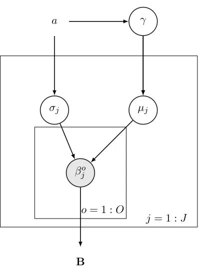
considering a set of related outcomes and drugs, e.g., heart-disease related outcomes and the set of drugs one might prescribe for heart-related conditions. We take a hierarchical Bayesian approach. By analogy with ridge regression, we use normal priors for the regression parameters (sparsifying priors such as the double exponential could be used instead). We shrink the coefficients for drugj for all outcomesotoµj by placing an independent normal

prior on eachβ_jo asβ_jo ∼ N(µj, σ2j),∀(j, o), where µj ∼ N(0, γ2),∀j. This prior helps with

numerical instability, overfitting, and makes the model more interpretable. We assume uniform priors for hyperparameters σj and γ as σj ∼ U(0, a),∀j and γ ∼ U(0, a), where

hyperparameter a is a user-defined constant, which can also be determined through cross-validation. A natural extension of this model (not explored here) would be to have drugs belong to certain classes of drugs, so that priors can be defined based on each class of drugs; similarly with outcomes. The posterior density is as follows:

Pr(B,µ,σ, γ|y, a) ∝Pr(y|B)×Pr(B|µ,σ)×Pr(µ|γ)×Pr(γ|a)×Pr(σ|a) (4)

∝Y

o

Y

i

Y

d∈Di

exp x>_idβo P

d0exp x>_id0βo

!y_id(o)

×Y

j

Y

o

N(β_jo|µj, σ2j) ×

Y

j

N(µj|0, γ2)×

Y

j

Pr(σj|a)× Pr(γ|a).

The negative log-posterior (which can be used for finding the MAP solution if desired) is:

L₁ =−log (Pr(B,µ,σ, γ|y, a)). The graphical representation of this model is shown in Figure 1.

4.2 Model 1 - One Level of Latent Factors

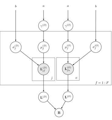
Two considerations motivate this model. First, modeling the full posterior distribution of Model 0 can be computationally expensive, particularly for largeN,J, andO, whereJ and O determine the number of variables to be estimated within the B matrix. Second, Model 0 overlooks the fact that drugs and outcomes might come from a smaller number of latent classes; for instance, there are commonly several drugs that are extremely similar to each other for treating a set of highly related illnesses. We consider F latent factors for drugs and outcomes. We model theJ×O matrixB asB=L(D)×L(O), where

L(D)= 

 

L(₁D_,1) ... L(₁D_,F)

: : :

L(_J,D₁) ... L(_J,FD) 

 ,L

(O)₌



 

L(₁O_,1) ... L(₁O_,O)

: : :

L(_F,O₁) ... L(_F,OO) 

 .

This way, we do not assume we know in advance which drugs have similar effects on which outcomes, instead we estimate this from data. The number of latent factors F can be determined by cross-validation. The total number of latent factors isJ×F+F×O, which can be substantially less thanJ×O. The coefficientβo_j associated with outcomeoand drug

j can be calculated as β_jo=

F

P

f=1

γ

µj

σj

β_jo a

B

j = 1 :J o= 1 :O

Figure 1: Graphical representation of Model 0

For drug latent factors, we place independent normal priors on the entries of L(D) as

L(_jfD)∼ N(µ(_fD), σ_f(D)2),∀(j, f), whereµ(_fD)∼ N(0, γ(D)2),∀f.

Similarly, we define normal priors on the entries ofL(O) as

L(_{f o}O)∼ N(µ(_fO), σ(_fO)2),∀(f, o), where µ(_fO)∼ N(0, γ(O)2),∀f.

We assume uniform priors for hyperparameters σj and γ as

σ_f(D) ∼U(0, a),∀f, σ_f(O) ∼U(0, a),∀f, γ(D)∼U(0, b), γ(O)∼U(0, b),

Pr(L(D),L(O),µ(D),µ(O),σ(D),σ(O), γ(D), γ(O)|y)∝Pr(y|L(D),L(O)) (5)

×Pr(L(D)|µ(D),σ(D))×Pr(L(O)|µ(O),σ(O))×Pr(µ(D)|γ(D))×Pr(µ(O)|γ(O))

×Pr(σ(D)|a)×Pr(σ(O)|a)×Pr(γ(D)|b)×Pr(γ(O)|b)

∝Y

o

Y

i

Y

d∈Do i

exp x>_idβo P

d0exp x>_id0βo

!y(_ido)

× J Y j=1 F Y f=1

N(L(_jfD)|µ_f(D), σ_f(D)2)×

F Y f=1 O Y o=1

N(L(_{f o}O)|µ_f(O), σ(_fO)2)

×

F

Y

f=1

N(µ(_fD)|0, γ(D)2)×

F

Y

f=1

N(µ(_fO)|0, γ(O)2)

× Pr(σ(_fD)|b)×Pr(σ(_fO))|b)×Pr(γ(D)|a)×Pr(γ(D)|a).

The graphical representation of this hierarchical Bayesian model is given in Figure 2.

4.3 Model 2 - Two Levels of Latent Factors Here we representB as

B=L(D)×L(F)×L(O),

where

B= 

 

L(₁D_,1) ... L(₁D_,F)

1

: : :

L(_J,D₁) ... L(_J,FD)

1   ×   

L(₁F_,1) ... L(₁F_,F)

2

: : :

L(_FF)

1,1 ... L

(F)

F1,F2

  ×   

L(₁O_,1) ... L(₁O_,O)

: : :

L(_FO)

2,1 ... L

(O)

F2,O



 .

The number of latent factors is thus J ×F1 +F1 ×F2+F2×O, which can be less than

the number of variables of Model 1 in many cases. Its major benefit is interpretability, since now the number of latent drug factors and the number of latent outcome factors can be estimated differently. L(D) represents the relationship between drugs and latent drug-related factors, L(F) represents the relationship between latent drug-related factors and latent health-outcome-related factors, and L(O) represents the relationship between latent health-outcome-related factors and health-outcome-related factors. L(F) is really the core set of variables since they relate the latent treatments to the latent health outcomes.

The priors are L(_jfD)

1 ∼ N(µ

(D)

f1 , σ

(D)2

f1 ), L

(O)

f2o ∼ N(µ

(O)

f2 , σ

(O)2

f2 ), L

(F)

f1f2 ∼ N(µ

(F)_{, σ}(F)2_),

µ(_fD)

1 ∼ N(0, γ

(D)2_{), µ}(F) _{∼ N(0, γ}(F)2_{), µ}(O)

f2 ∼ N(0, γ

(O)2_{), σ}(D)

f1 ∼ U(0, a), σ

(F) _∼

U(0, a), σ(_fO)

2 ∼ U(0, a), γ

(D) _{∼ U(0, b), γ}(F) _{∼ U(0, b), and γ}(O) _{∼ U(0, b) for all}

b a a b

γ(D) γ(O)

µ(_fD) µ(_fO)

σ_f(D) σ_f(O)

L(_jfD) L(_{f o}O)

L(D) L(O)

B

f = 1 :F o

j

Figure 2: The Graphical Framework for Hierarchical Bayesian Model with one level of latent factors

The posterior density is

Pr(L(D),L(F),L(O),µ(D),µ(F),µ(O),σ(D),σ(F),σ(O), γ(D), γ(F), γ(O)|y) (6) ∝Pr(y|L(D),L(F),L(O))×Pr(L(D)|µ(D),σ(D))×Pr(L(F)|µ(F),σ(D))×Pr(L(O)|µ(O),σ(O)) ×Pr(µ(D)|γ(D))×Pr(µ(F)|γ(F))×Pr(µ(O)|γ(O))

×Pr(σ(D)|a)×Pr(σ(F)|a)×Pr(σ(O)|a)×Pr(γ(D)|b)×Pr(γ(F)|b)×Pr(γ(O)|b).

Table 1 compares the number of parameters in each of the three models. Models 1 and 2 have much fewer parameters when F, F1, and F2 are lower than J and O. We use

Model Name # of Parameters # of Hyperparameters Total

Model 0 J∗O 2∗J+ 1 J∗O+ 2∗J+ 1

Model 1 J∗F+F∗O 4∗F+ 2 J∗F+F∗O+ 4∗F+ 2

Model 2 J∗F1 +F1∗F2 +F2∗O 2∗F1+ 2∗F2+ 5 J∗F1+F1∗F2 +F2∗O+ 2∗F1+ 2∗F2+ 5

Table 1: The number of parameters and hyperparameters in each model.

Jt(x, x0) which proposes a new parameter set x0 given the current parameter set x. We

denote Θas the set of all parameters in the model excludingB.

Step 1. Generate an initial state {B0,Θ0}with positive probability Pr(B0,Θ0|y) and set t= 1.

Repeat the following until stationary distribution and the desired number of samples are reached considering optional burn-in and/or thinning.

Step 2. Sample {B∗,Θ∗} from the symmetric proposal distribution

Jt({Bt−1,Θt−1},{B∗,Θ∗}).

Step 3. Calculate the acceptance probability

α= min

1, Pr(B

∗_,Θ∗_|y)

Pr(Bt−1_,Θt−1_|y)

.

Step 4. Draw a random number u from Unif(0,1). If u ≤ α, accept the proposal state

{B∗,Θ∗}and set Bt=B∗,Θt=Θ∗, else set Bt=Bt−1,Θt=Θt−1. Sett:t+ 1.

Our implementation uses a component-wise sampling approach. For truly large-scale applications, blocked sampling approaches may be necessary.

5. Simulation Study

β1,1

-2.6 -2.4 -2.2

0 0.2 0.4

β1,2

-1.3 -1.2 -1.1

0 0.2 0.4

β1,3

-2 -1.8 -1.6

0 0.2 0.4

β1,4

-2.5 -2 -1.5

0 0.2 0.4

β2,1

1.15 1.2 1.25

0 0.2 0.4

β2,2

0.6 0.7 0.8

0 0.2 0.4

β2,3

0.6 0.7 0.8

0 0.2 0.4

β2,4

1.5 1.6 1.7

0 0.2 0.4

β3,1

1.6 1.65 1.7

Posterior density

0 0.2 0.4

β3,2

1.6 1.65 1.7

0 0.2 0.4

β3,3

0.8 0.9 1

0 0.2 0.4

β3,4

-1 -0.9 -0.8

0 0.2 0.4

β4,1

-0.6 -0.5 -0.4

0 0.2 0.4

β4,2

0.3 0.4 0.5

0 0.2 0.4

β4,3

-1 -0.8 -0.6

0 0.2 0.4

β4,4

-0.3 -0.2 -0.1

0 0.2 0.4

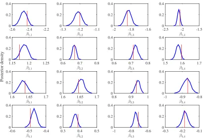
Figure 3: Normalized histograms of posterior samples for each element of B in Model 0. The vertical line indicates the true value.

6. Application to Blood Glucose Analysis for Diabetes

True values -2.6 -1.6 -0.6 0.4 1.4

Posterior mean

-2.6 -1.6 -0.6 0.4 1.4

2 a) Model 0

True values

-1.2 -0.8 -0.4 0

Posterior mean

-1.2 -0.8 -0.4 0

b) Model 1

True values -1.5 -1 -0.5 0 0.5

Posterior mean

-1.5 -1 -0.5 0 0.5

c) Model 2

Figure 4: Scatter plot of posterior means vs. true parameter values of elements of B for Models 0, 1 and 2.

Time

6:00 8:00 10:00 12:00 14:00 16:00 18:00 20:00 22:00

More-than-usual

exercise activity Less-than-usualmeal ingestion NPH injection

Pre-lunch BG measurement

(60 mg/dl)

Pre-lunch BG measurement

(47 mg/dl) NPH injection

Pre-breakfast BG measurement

(135 mg/dl)

Pre-snack BG measurement (118 mg/dl) Measurements

Events

Figure 5: Sample longitudinal traces for a patient with multiple drug/treatments exposures and blood glucose measurements over a day. Downwards arrows indicate glucose measurements. Upwards arrows indicate treatments.

We will describe the setup in more detail:

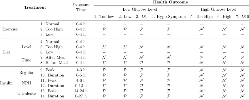
onset (O), time of peak action (P), and effective duration (D). The exposure time intervals for peak, and duration used in this paper, which were provided with the data set, are shown in Table 2 in the “Exposure Time” column in the bottom several rows of the table labeled “Insulin.”

Treatment Exposure

Time

Health Outcome

Low Glucose Level High Glucose Level

1. Too low 2. Low 3.D1 4. Hypo Symptom 5. Too High 6. High 7.D10

Exercise

1. Normal 0-4 h − − − − − − −

2. Too High 0-4 h P P P P N N N

3. Low 0-4 h − − − − − − −

Diet

Level

4. Normal 0-4 h − − − − − − −

5. Too High 0-4 h N N N N N N N

6. Low 0-4 h − − − − − − −

Time 7. After Meal 0-4 h N N N N P P P

8. Before Meal 0-4 h P P P P N N N

Insulin

Regular 9. Peak 1-3 h P P P P N N N

10. Duration 0-5 h P P P P N N N

NPH 11. Peak 4-6 h P P P P N N N

12. Duration 0-12 h P P P P N N N

Ultralente 13. Peak 14-24 h P P P P N N N

14. Duration 0-27 h P P P P N N N

Table 2: The list of drugs/treatments and health outcomes and their known correlations.

P means strong positive correlation, andN means strong negative correlation,D1 is lower decile andD10 means highest decile.

Based on the actual time of injection, we determined the intervals at which the patient is at peak and/or within the duration of an insulin injection. Based on this, six types of treatments were considered, (1) regular insulin on peak, (2) regular insulin on duration, (3) NPH insulin on peak, (4) NPH insulin on duration, (5) Ultralente insulin on peak, and (6) Ultralente insulin on duration. At each interval of time, the patient can be either insulin free or subject to one of the above six exposures.

The second class of treatment is exercise, which may have complex effects on the glu-cose level. For example, gluglu-cose levels can fall during exercise but also quite a few hours afterwards. Three types of exercise are reported, (1) normal exercise, (2) lower than nor-mal exercise, and (3) higher than nornor-mal exercise. Each type of exercise was considered separately as a single treatment.

Based on all of the treatments described, the total number of variables associated with treatments in the model is 14 (J = 14). The variables are all listed on Table 2 in the “Treatment” column on the left.

Health Outcomes. The outcomes are divided into categories, based on glucose level. Given that normal pre-meal blood glucose ranges from approximately 80-120 mg, and post-meal blood glucose ranges from 80-140 mg/dl (Bache and Lichman, 2013), we considered seven health outcomes for glucose level: extremely low (below 40 mg/dl), low (between 40-80 mg/dl), high (over 140 mg/dl), extremely high (over 180 mg/dl), lower decile (lower 10% of glucose level for each patient), upper decile (upper 10% of glucose level for each patient), and hypoglycemic (low glucose) symptoms. Thus, the total number of outcomes considered for our analysis is O = 7. We can perform an evaluation only on intervals where we have glucose measurements, thus we only use those intervals. Note that more than one outcome can occur in each interval.

True Relationships Between Drugs and Outcomes. We wanted to determine whether our model reproduces known relationships between treatments and glucose levels from the data alone. The information about true relationships within Table 2 mainly come from material accompanying the data set and www.diabetes.org. We denoted known positive effects in Table 2 byP, strong negative effects byN, and relationships that were unknown were denoted by dashes “–”. For example, we expect NPH injection on peak to decrease the likelihood of having “Too High” glucose level, so the correlation between NPH on peak and “Too High” glucose level is known to be negative (N).

Mixing. We performed cross-validation, dividing our data into five folds, training our models on four folds and testing on the fifth. We removed the first 5000 iterations (as burn-in) of Metropolis-Hastings sampling, and obtained 6000 additional samples to estimate the posterior. Figure 6 shows samples from the posterior of one of the variables, β_{NPH on peak}Too high GL, for five separate model instantiations (Model 0, Model 1 with F=2, Model 1 with F=3, Model 2 with F1 = 2, F2 = 2, and Model 2 with F1 = 3, F2 = 3. Recall that in Models 1

and 2, we sample elements of the matrices of latent factors and then calculateB. From this figure, we observe reasonable mixing for all models, and we observe that models with latent factors (Models 1 and 2) have better mixing and convergence, possibly due to the smaller number of variables.

5000 20000 30000 40000 50000

Model 0

-0.3 -0.2 -0.1 0

-0.25 -0.2 -0.15 -0.1 -0.05 0

0 500 1000

5000 2000 30000 4000 50000

Model 1 F=2

-0.3 -0.2 -0.1 0

-0.25 -0.2 -0.15 -0.1 -0.05 0

0 500 1000

5000 20000 30000 40000 50000

Model 1 F=3

-0.3 -0.2 -0.1 0

-0.25 -0.2 -0.15 -0.1 -0.05 0

0 500 1000

5000 20000 30000 40000 50000

Model 2 F 1

=2, F

2

=2

-0.3 -0.2 -0.1 0

-0.2 -0.15 -0.1 -0.05 0

0 500 1000

Iteration No.

5000 20000 30000 40000 50000

Model 2 F 1

=3, F

2

=3

-0.3 -0.2 -0.1 0

-0.25 -0.2 -0.15 -0.1 -0.05 0

0 500 1000

Figure 6: Samples from the posterior ofβ_{NPH on peak}Too high GL for five model instantiations (left), and their histograms (right). The first 5000 samples were discarded as burn-in. We observe better mixing and convergence in the models with latent factors (Model 1 and Model 2).

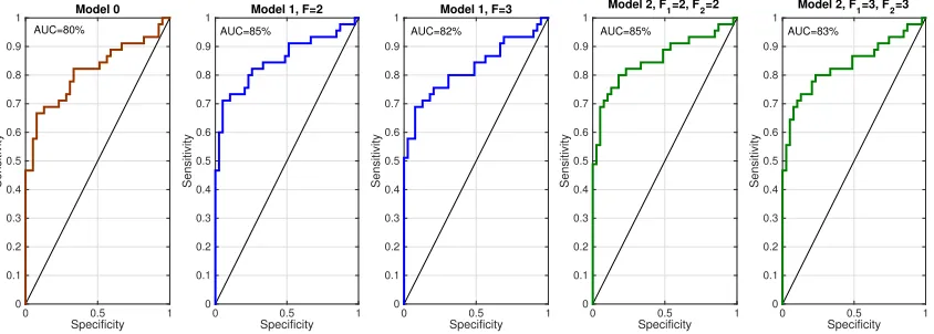
the ranking, and calculating the true positive rate and false positive rate with respect to the true coefficients. We computed these ROC curves for all five model instantiations to obtain Figure 8. These ROC curves indicate that all models performed well, in the sense of estimating reasonable signs for the coefficients. The curves also indicate that models with more latent factors performed better than Model 0. The models with two latent treatment and outcome factors performed slightly better than the models with three latent treatment and outcome factors, though there was no significant difference in performance between Model 1 and Model 2 for the same number of latent treatment and outcome factors. Drug Surveillance. We evaluated prediction performance of our model as follows: for each patient we calculated the Poisson rate of each condition at each hour considering all drug exposures. For each condition, we then checked whether or not the patient had the condition at that time. The Poisson rate acts as the score of each patient with regards to each condition. In Figure 9, we present the actual glucose level for a patient at 20 measurement points (upper figure) as well as the estimated intensity rate of the Too-High glucose level for the same patient (lower figure). Each point in this figure represents the estimated x>_idβˆo_{, where ˆβ}o _{are the estimated regression coefficients associated with}

Number of parameters

40 60 80 100 120 140

CPU time (hours)

1.5 2 2.5 3 3.5 4 4.5 5 5.5 6 Model 1 F=3 Model 2 F

1=2, F2=2

Model 2 F

1=3, F2=3

Model 1 F=2

Model 0

Figure 7: Comparison between the CPU time and number of variables in the five model instantiations. Model 0 has larger number of variables and significantly higher CPU time.

Specificity

0 0.5 1

Sensitivity 0 0.1 0.2 0.3 0.4 0.5 0.6 0.7 0.8 0.9

1 Model 0

Specificity

0 0.5 1

Sensitivity 0 0.1 0.2 0.3 0.4 0.5 0.6 0.7 0.8 0.9

1 Model 1, F=2

Specificity

0 0.5 1

Sensitivity 0 0.1 0.2 0.3 0.4 0.5 0.6 0.7 0.8 0.9

1 Model 1, F=3

Specificity

0 0.5 1

Sensitivity 0 0.1 0.2 0.3 0.4 0.5 0.6 0.7 0.8 0.9 1

Model 2, F₁=2, F₂=2

Specificity

0 0.5 1

Sensitivity 0 0.1 0.2 0.3 0.4 0.5 0.6 0.7 0.8 0.9 1

Model 2, F₁=3, F₂=3

AUC=80% AUC=85% AUC=82% AUC=85% AUC=83%

Figure 8: Receiver Operating Characteristic (curve) for evaluating the signs of coefficients against true signs for five model instantiations. See the text for details of how these curves were generated.

analysis for Too-Low glucose level. It can be observed from this figure that the times where this coefficient is particularly large are the same times where the glucose level drops substantially. This kind of dramatic agreement was not observed for all patients nor all conditions, so below we describe a more general evaluation procedure.

Measurement #

0 2 4 6 8 10 12 14 16 18 20

Glucose Level

50 100 150 200 250 300 350

Patient # 1

Measurement #

0 2 4 6 8 10 12 14 16 18 20

Estimated Intensity for _{Too High Glucose level} -0.8 -0.6 -0.4 -0.2 0 0.2

Figure 9: Monitoring Too-High glucose levels over 20 hours. The upper figure shows the true glucose levels obtained by measurement, and the lower figure shows the estimated

x>_idβˆo _{for the Too-High glucose outcome over 20 consecutive measurements.}

Measurement #

0 2 4 6 8 10 12 14 16 18 20

Glucose Level

0 50 100 150 200

250 Patient # 1

Measurement #

0 2 4 6 8 10 12 14 16 18 20

Estimated Intensity

Too low Glucose Level -2 -1.5 -1 -0.5 0 0.5 1

Figure 10: Monitoring too-low glucose levels over 20 hours. The upper figure shows the true glucose levels obtained by measurement, and the lower figure shows the estimatedx>_idβˆo _{for the too-low glucose outcome over 20 hours.}

timing of the drugs recently taken by the patient. The results were consistent across all five model instantiations.

Normal Too Low

Normalized Rate 0 0.2 0.4 0.6 0.8 1 Model 0

Normal Too High

Normalized Rate 0 0.2 0.4 0.6 0.8 1 Model 0

Normal Too Low

0 0.2 0.4 0.6 0.8 1

Model 1, F=2

Normal Too High

0 0.2 0.4 0.6 0.8 1

Model 1, F=2

Normal Too Low

0 0.2 0.4 0.6 0.8 1

Model 2, F₁ = F₂ = 2

Normal Too High

0 0.2 0.4 0.6 0.8 1

Model 2, F₁ = F₂ = 2

Normal Too Low

0 0.2 0.4 0.6 0.8 1

Model 1, F=3

Normal Too High

0 0.2 0.4 0.6 0.8 1

Model 1, F=3

Normal Too High

0 0.2 0.4 0.6 0.8 1

Model 2, F₁ = F₂ = 3

Normal Too Low

0 0.2 0.4 0.6 0.8 1

Model 2, F₁ = F₂ = 3

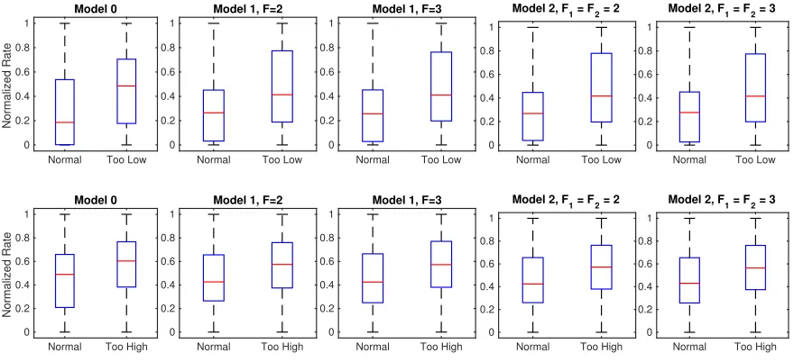
Figure 11: Comparison between the box-plots for Too-High and Too-Low glucose levels and the normal condition for all five model instantiations, where the Poisson rates were normalized for each person.

In Table 3, we report an AUC (area under the ROC curve) value that measures the probability that a method ranks a positive condition timepoint higher than a timepoint with no condition, for the same patient. In particular, we are testing whether the Poisson rate of a patient with a health condition is higher than the estimated rate of the same patient when no condition is present. For each model instantiation, we trained the model on four training folds and then calculated the AUC on the fifth fold, and we repeated this for each condition. We reported the average and standard deviation of AUC over all patients in the test sets. Again D1 is the lower decile (lower 10% of glucose level for each patient), and D10 is the upper decile (upper 10% of glucose level for each patient).

Intuition of B as compared with other methods. We compared the performance of the proposed models with that of the univariate self-controlled case series (SCCS), and multi-variate self-controlled case series (MSCCS) (Simpson et al., 2013) with and without an`2 regularization term on the coefficients. For each model instantiation and each method,

Too low Low Too high High D1 D10 Hypo Symptom

Model 0 Mean 70.30% 62.92% 62.98% 61.26% 58.20% 56.39% 59.17% sd 9.56% 2.79% 3.38% 2.70% 3.93% 3.51% 4.95%

Model 1,F= 2 Mean 70.86% 62.70% 63.06% 61.58% 57.97% 56.05% 56.71% sd 8.28% 2.47% 3.14% 2.11% 3.36% 3.04% 3.19%

Model 1,F= 3 Mean 70.66% 62.68% 62.92% 61.51% 57.97% 56.35% 56.33% sd 7.89% 2.52% 3.14% 2.12% 3.37% 2.90% 2.87%

Model 2,F1=F2= 2

Mean 70.19% 62.71% 62.97% 61.44% 58.00% 55.91% 56.88% sd 9.51% 2.43% 3.18% 2.13% 3.34% 3.06% 3.02%

Model 2,F1= 3, F2= 3

Mean 70.07% 62.73% 62.99% 61.47% 58.05% 56.05% 56.68% sd 9.52% 2.44% 3.16% 2.07% 3.31% 3.05% 2.79%

Table 3: Average and standard deviation (sd) of AUC over 5 folds. The entities that were ranked for each AUC calculation are measurements for a patient including time points when the patient had a condition and time points when the patient did not have a condition. The AUC indicates whether our method ranks a randomly chosen time point where a patient had a condition higher than a randomly chosen time point where a patient did not have a condition.

MSCCS, and all FSCCS Bayesian model instantiations (Model 0-2) performed better than all of the traditional models, yielding higher AUC’s and better agreement in the mean signs of coefficients; further the standard deviations for the coefficient values were substantially lower. These performance benefits come in addition to the other benefits discussed earlier, including computational tractability and interpretability of the latent factors.

Measure Method

Model 0 Mode1 F= 2

Model 1 F= 3

Model 2 F1= 2, F2= 2

Model 2 F1= 3, F2= 3

SCCS MSCCS Regularized MSCCS

AUC 0.813 0.852 0.824 0.856 0.836 0.693 0.773 0.774

B−

Mean -0.190 -0.281 -0.276 -0.278 -0.282 -0.492 -0.663 -0.349

Median -0.077 -0.136 -0.143 -0.130 -0.141 -0.047 -0.122 -0.122

sd 0.353 0.417 0.410 0.422 0.424 2.362 2.462 0.640

B+

Mean 0.071 0.099 0.096 0.105 0.096 -0.552 -0.561 -0.023

Median 0.030 0.103 0.111 0.106 0.106 0.065 0.126 0.125

sd 0.368 0.369 0.385 0.368 0.378 3.158 3.149 0.771

7. Concluding Remarks

The novel elements of this work are as follows. (1) We estimate the effects of many drugs on many health outcomes simultaneously. Borrowing strength across similar drugs and outcomes allows us to create better estimates across both drugs and outcomes. (2) We use latent factors to encode latent classes of drugs and outcomes, to help with interpretability, and to provide a computational benefit. Another type of computational benefit is provided naturally by using the SCCS’s framework, since we do not need to estimate the baseline rates of outcomes for each patient. This approach is scalable to large longitudinal observational databases, is applicable to problems beyond healthcare, and provides a level of interpretabil-ity to physicians and patients that was not previously possible. Fully Bayesian inference via MCMC may not be feasible for truly large-scale problems. Recent developments in cyclic coordinate descent algorithms (see, for example, in Suchard et al., 2013b) would apply in our context and represent one possible approach for very scale MAP estimation.

Acknowledgments

Appendix A. Figures 12 and 13.

β1

,1

-0.9 -0.8 -0.7

0 0.2 0.4

β1

,3

-1.2 -1 -0.8

0 0.2 0.4

β1

,4

-0.8 -0.7 -0.6

0 0.2 0.4

β2,1

-1.2 -1 -0.8

Posterior density

0 0.2 0.4

β2,2

-0.550 -0.5 -0.45 -0.4

0.2 0.4

β2,3

-1.2 -1 -0.8

0 0.2 0.4

β2,4

-1 -0.8 -0.6

0 0.2 0.4

β3,1

-0.4 -0.2 0

0 0.2 0.4

β3,2

0 0.1 0.2

0 0.2 0.4

β3,3

-0.6 -0.5 -0.4

0 0.2 0.4

β3,4

-0.3 -0.2 -0.1

0 0.2 0.4

β4

,1

-1.1 -1 -0.9

0 0.2 0.4

β4

,2

-0.6 -0.55 -0.5 -0.45

0 0.2 0.4

β4

,3

-1.2 -1 -0.8

0 0.2 0.4

β4

,4

-1 -0.9 -0.8

0 0.2 0.4 β1,1

-0.4 -0.35 -0.3 -0.25 0

0.1 0.2 0.3

Figure 12: Normalized histograms of posterior samples for each element of B in Model 1. The vertical line indicates the true value.

β1

,1

0.4 0.5 0.6

0 0.2 0.4

β1

,3

-1.5 -1.4 -1.3

0 0.2 0.4

β1

,4

-1 -0.9 -0.8

0 0.2 0.4

β2,1

0.5 0.6 0.7

Posterior density

0 0.2 0.4

β2,2

-0.6 -0.55 -0.5 -0.45

0 0.2 0.4

β2,3

-0.9 -0.8 -0.7

0 0.2 0.4

β2,4

-0.5 -0.4 -0.3

0 0.2 0.4

β3,1

0.4 0.5 0.6

0 0.2 0.4

β3,2

-0.250 -0.2 -0.15 -0.1

0.2 0.4

β3,3

-0.4 -0.3 -0.2

0 0.2 0.4

β3,4

-0.2 -0.1 0

0 0.2 0.4

β4

,1

-0.5 -0.4 -0.3

0 0.2 0.4

β4

,2

0.25 0.3 0.35

0 0.2 0.4

β4

,3

0.4 0.5 0.6

0 0.2 0.4

β4

,4

0.1 0.2 0.3

0 0.2 0.4 β1,2

-1.2 -1.1 -1 -0.9 0

0.1 0.2 0.3

References

K. Bache and M. Lichman. UCI Machine Learning Repository, University of California, Irvine, School of Information and Computer Sciences, 2013.

E.I. Benchimol, S. Hawken, J.C. Kwong, and K. Wilson. Safety and utilization of influenza immunization in children with inflammatory bowel disease. Pediatrics, 131(6):1811–1820, 2013.

C.M. Carvalho, J. Chang, J.E. Lucas, J.R. Nevins, Q. Wang, and M. West. High-dimensional sparse factor modeling: applications in gene expression genomics.Journal of the American Statistical Association, 103(484), 2008.

C.S.L. Chui, K.K.C. Man, C.L. Cheng, E.W. Chan, W.C.Y. Lau, V.C.C. Cheng, D.S.H. Wong, Y.H. Yang Kao, and I.C.K. Wong. An investigation of the potential association between retinal detachment and oral fluoroquinolones: A self-controlled case series study. Journal of Antimicrobial Chemotherapy, 69(9):2563–2567, 2014.

M.C. Cobanoglu, C. Liu, F. Hu, Z.N. Oltvai, and I. Bahar. Predicting drug-target inter-actions using probabilistic matrix factorization. Journal of Chemical Information and Modeling, 53(12):3399–3409, 2013.

P. Farrington. Relative incidence estimation from case series for vaccine safety evaluation. Biometrics, 51:228–235, 1995.

P. C. Farrington, K. Anaya-Izquierdo, H.J. Whitaker, M.N. Hocine, I. Douglas, and L. Smeeth. Self-controlled case series analysis with event-dependent observation peri-ods. Journal of the American Statistical Association, 106(494), 2011.

J. Ghosh and D.B. Dunson. Default prior distributions and efficient posterior computation in Bayesian factor analysis. Journal of Computational and Graphical Statistics, 18(2): 306–320, 2009.

S.K. Greene, M. Kulldorff, R. Yin, W.K. Yih, T.A. Lieu, E.S. Weintraub, and G.M. Lee. Near real-time vaccine safety surveillance with partially accrued data. Pharmacoepidemi-ology and Drug Safety, 20(6):583–590, 2011.

D. Madigan, P. Ryan, S.E. Simpson, and I. Zorych. Bayesian methods in pharmacovigilance, volume 9. Oxford University Press, 2010.

D. Madigan, S. Simpson, W. Hua, A. Paredes, B. Fireman, and M. Maclure. The self-controlled case series: Recent developments, 2011.

D. Madigan, P.E. Stang, J.A. Berlin, M. Schuemie, J.M. Overhage, M.A. Suchard, B. Du-mouchel, A.G. Hartzema, and P.B. Ryan. A systematic statistical approach to evaluating evidence from observational studies. Annual Review of Statistics and Its Application, 1: 11–39, 2014.

SE. Simpson. A positive event dependence model for self-controlled case series with appli-cations in postmarketing surveillance. Biometrics, 69(1):128–136, 2013.

S.E. Simpson, D. Madigan, I. Zorych, M.J. Schuemie, P.B. Ryan, and M.A. Suchard. Mul-tiple self-controlled case series for large-scale longitudinal observational databases. Bio-metrics, 69(4):893–902, 2013.

MA. Suchard, I. Zorych, SE. Simpson, MJ. Schuemie, PB. Ryan, and D. Madigan. Em-pirical performance of the self-controlled case series design: lessons for developing a risk identification and analysis system. Drug Safety, 36(1):83–93, 2013a.

Marc A. Suchard, Shawn E. Simpson, Ivan Zorych, Patrick Ryan, and David Madigan. Massive parallelization of serial inference algorithms for a complex generalized linear model. ACM Transactions on Modeling and Computer Simulation (TOMACS), 23(1):10, 2013b.

H. J. Whitaker, C. P. Farrington, B. Spiessens, and P. Musonda. Tutorial in biostatistics: the self-controlled case series method. Statistics in Medicine, 25(10):1768–1797, 2006.